The Determinants of Bank
Lending in Commercial Banks
Trabalho Final na modalidade de Dissertação apresentado à Universidade Católica Portuguesa para obtenção do grau de mestre em Business Economics
por
Joana Isabel Pereira da Rocha
sob orientação deProfessor Ricardo Miguel Martins da Costa Ribeiro
Católica Porto Business School Março 2017
ii
Resumo
Esta tese desenvolve e estima um modelo de procura de forma a avaliar os determinantes da escolha dos consumidores de serviços de empréstimos bancários em bancos comerciais. De acordo com a literatura de escolha discreta, os consumidores respondem tipicamente ao preço e às características dos produtos. Utilizando dados do setor bancário dos E.U.A. de 2011 a 2015, os resultados sugerem que os consumidores respondem negativamente a um aumento nas comissões de serviço e nas taxas de juro. Além disso, indicam que os consumidores preferem bancos mais recentes e que o risco de crédito do banco não influencia o processo da tomada de decisão.
Palavras-chave: estimação da procura; produtos diferenciados; escolha discreta; risco de crédito; setor bancário.
iv
Abstract
This thesis develops and estimates a demand model for commercial bank loan services to assess the determinants of consumer bank lending choice involving commercial banks. Following the discrete choice literature, consumers typically respond to price and product characteristics. Using data from the U.S. banking industry from 2011 to 2015, the results suggest that consumers respond negatively to an increase in service fees and in loan interest rates. Furthermore, they indicate that consumers prefer younger banks and that asset risk does not influence the decision-making process.
Keywords: demand estimation; product differentiation; discrete choice; asset risk; banking industry.
Index
Resumo ... ii
Abstract ... iv
Index ... vi
Table Index ... viii
Introduction ... 10
1. Literature Review ... 13
1.1. Empirical Framework ... 13
1.2. Estimation Procedure ... 15
2. Empirical Framework ... 16
2.1. Definitions for a model of loan services demand ... 16
2.2. Demand model ... 18 2.3. Estimation Procedure ... 24 3. Data Description ... 28 3.1. Data Sources ... 28 3.2. Explanatory Variables ... 29 3.3. Instrumental Variables ... 31 3.4. Summary Statistics ... 33 4. Estimation Results ... 34 4.1. Literature Comparison... 38 4.2. Asset Risk ... 38 4.3. Price elasticities ... 39 5. Conclusion ... 40 Bibliography ... 42
viii
Table Index
Table I – Summary Statistics... 34 Table II – Demand Estimation Results ... 37 Table III – Price Elasticities ... 40
10
Introduction
United States (U.S.) bank loans are experiencing the fastest annual expansion since 2007, which may be a sign of greater confidence, but also that lenders are taking too much risk. The Eurozone is experiencing a different scenario since there policymakers’ efforts to promote lending to businesses have hardly succeeded. It is common knowledge that lending is the primary source of revenue for banks and, therefore, it is only natural that, on one hand, banks may take too much risk and, on the other hand, regulators intend to discourage the amount of risk that banks take.1
This thesis develops and estimates a demand model for commercial bank loan services to assess the determinants of bank lending choice in commercial banks, with a particular focus in evaluating the impact of banks’ asset risk policies on U.S. bank lending. Although the thesis examines the U.S. banking market, I believe that its main findings, concerning the determinants of bank lending, may be valid for commercial banks in other countries. This belief is corroborated by the fact that empirical studies across a variety of different countries tend to use the same set of bank characteristics when estimating demand for bank services.
Bank loan services constitute a differentiated product. Different banks offer slightly different substitute loan services. As a consequence, in order to estimate a demand model for loan services, I will follow the discrete choice literature (Berry, 1994; Berry, Levinsohn and Pakes, 1995) and modelled investor decisions as a function of loan prices and bank characteristics. The proposed model is estimated for the U.S. commercial banking sector over 2011-2015, using a data set
that combines information from one specific website, usbanklocations.com. In particular, the loan prices will be decomposed into service fees and loan interest rate, and the set of bank characteristics will be the number of branches, the bank’s age, the number of employees per branch, the asset risk and the number of states in which a bank operates. This work departs from the existing literature since, to the best of my knowledge, a demand model for loan services has not yet been applied to the U.S. commercial banking industry and asset risk has not been incorporated in the set of bank characteristics.
The results suggest that the consumers decision-making process concerning bank lending is influenced by (i) loan interest rates, (ii) service fees, and (iii) bank age. All other characteristics, including bank asset risk, seem not to affect this process. Further, the results also suggest that consumer choice is inelastic with respect to service fees, suggesting that banks have considerable market power, but choose not to abuse it.
The remainder of the thesis is organized as follows. Section 1 provides a literature review on demand estimation in the banking industry. In Section 2, the empirical framework is outlined, including the main definitions and the demand model itself. In Section 3, the data and the estimation procedures are presented. Section 4 presents the results and, finally, section 5 concludes.
1. Literature Review
1.1. Empirical Framework
The banking industry literature supports the decision to follow a discrete choice approach (Dick, 2008; Molnár, Márton and Csilla, 2006; Nakane, Alencar and Kanczuk, 2006; Brito, Pereira and Ribeiro, 2008). In particular, the decision to estimate standard and nested multinomial logit demand models. Dick (2008) was the first to apply a structural demand model based on consumer choice under product differentiation on retail deposit services, and most of the subsequent literature adopts her framework.
Dick (2008) estimates a demand model for deposit services using data on U.S. commercial banks to examine (i) what characterizes consumer behaviour in banking services, (ii) what are the levels of competition in the industry, and (iii) how does consumer welfare get affected by policy changes (for example, the deregulation of bank’s geographic scope). As discussed above, Dick (2008) follows a discrete choice literature where consumer decisions are based on prices and a set of bank characteristics. Therefore, she estimates a standard multinomial logit model and a nested logit model. In the latter she groups banks into those that operate in more than one state and those that operate in exactly one state. She decomposes price into service fees and deposit interest rate, thus in this framework it is natural to assume that, on one hand, if service fees increase, the demand for deposits will decrease and so will the investors’ utility, and, on the other hand, if the deposit interest rate increases the demand for deposits will also increase and so will the investors’ utility. Regarding the observed bank characteristics, she includes in the analysis variables that are observed at the bank level and at the bank-market level, and that are assumed to be important and
14
perceptible to the consumer. Thus, the observed bank characteristics are: the number of local branches per square mile; the number of employees per branch, which may be correlated with the waiting time; bank size (measured discretely as large, medium or small), that may capture the perceived service quality and the lower probability of failure attached to larger banks; the number of states in which the bank has presence, which may measure the value attached to network size and geographic diversification; and bank age, which may be a proxy for experience and expertise. Moreover, Dick (2008) incorporates control variables for demographic differences across local markets, such as income per capita and population density, and interacts them with the bank characteristics. The intention is to explore if consumers in more populated areas value more the number of branches in the local market.
Molnár, et al. (2006) estimate a demand model for deposit and loan services using data on Hungarian commercial banks to examine the degree of competition in the Hungarian household credit and deposit markets. They also decompose price into service fees and, deposit or loan interest rate, and include Dick (2008)’s set of bank characteristics, at the national-level, with the major difference being the fact that they use bank size as nests, while Dick (2008) uses it as a characteristic and nests the banks into those that are geographically diversified (by operating in more than one state) and those that have branches in exactly one state.
Nakane, et al. (2006) estimate a demand model for deposit and loan services using data on Brazilian commercial banks to examine the degree of competition in the Brazilian banking industry. They also separate price into service fees and, deposit and loan interest rates. However, regarding the bank characteristics, their approach is slightly different from Dick (2008) and from Molnár et al. (2006) since
they use bank characteristics at two levels: characteristics at the market-level (in their application, municipality) and characteristics at the country level. The observable market-level bank characteristics are: the number of bank branches in the municipality, the number of ATMs in the municipality, the branch density in the municipality, and the ATM density in the municipality. The observable country-level characteristics are: the number of bank branches in the country, the number of ATMs in the country, the number of states where the bank operates, bank age, the number of bank employees, the average number of bank employees per branch, and advertisement costs. Both Dick (2008) and Nakane, et al. (2006) use variables to control for demographic differences across local markets. While Dick (2008) interacts bank characteristics with income and population, Nakane,
et al. (2006) interact bank characteristics with municipality-level GDP per capita
and use, as control variables, municipality-level GDP, GDP per capita, geographic area, and population density.
1.2. Estimation Procedure
In this framework, as discussed above, price can be decomposed into two variables: loan interest rates and service fees. Both are charged to a consumer that is willing to buy a bank’s service and it is natural to assume that if they increase, the demand for loans will decrease and so will the investors’ utility. This brings us to the endogeneity problem that arises in the estimation of the models above. Due to the fact that not all bank characteristics are observed by the researcher and price variables may be correlated with these unobserved characteristics. Dick (2008) states that these variables can be the bank’s service quality, reputation linked to its soundness as a financial institution, prestige and expertise but also the ability to counter systemic financial distress. Therefore, banks with better unobserved characteristics may charge consumers more for this attribute. As a consequence, the price variables need to be instrumented. Molnár, et al. (2006)
16
and Nakane, et al. (2006) follow Dick (2008)’s approach in using cost shifters and Berry, Levinsohn and Pakes (1995) (hereafter BLP)’s, suggestion as instruments for price. Cost shifters denote direct cost variables, product mix, and balance sheet structure variables. The idea of using cost shifters as instruments, is that, a bank’s cost of operating may impact the bank’s pricing decisions, however it is not expected that they have a significant quality component, in other words, they are not expected to be correlated with the unobserved bank characteristics. BLP’s suggestion consists of using the characteristics of other products in the market as instruments for price. The reasoning behind this approach is that given the location of products in the characteristic space, price will be correlated with the characteristics of other products and therefore products that have close substitutes will have lower markups, while other products located further away from rival ones will have higher prices relative to cost.
2. Empirical Framework
2.1. Definitions for a model of loan services demand
Consumer decision:Consumers are expected to value and to be able to recognize several bank attributes when searching for a loan service. Though price might be considered the most relevant characteristic, also the overall quality and effectiveness of the service such as the waiting time or the perceived expertise and experience of a certain bank, may influence the consumer decision-making process.
Consumers:
The demand model focuses on loan services, which include real estate loans, farm loans, commercial and industrial loans, loans to individuals and all other
loans and leases. Therefore, the analysis includes the decisions of two types of consumers in the banking industry: households and nonfinancial businesses. Further, these consumers can be national or international, since the data aggregated loans from both domestic offices and non-U.S. addresses.
Commercial bank competitors:
Regulators classify the institutions that offer financial services into depositary and non-depositary institutions. Depositary institutions such as commercial banks, thrifts, savings banks and credit unions offer loan services by lending the money saved by depositors. Non-depositary institutions include finance companies, brokerages, mortgage lenders and venture capital firms.
Due to data limitations, only commercial banks will be considered, some of which will be modelled as inside options while some of which will be modelled, in aggregated terms, as the outside option. A commercial bank is included in the inside options if it accounted for at least one quarter of one percent in one of the years (to be defined below).
Output Quantity:
The output quantity a bank “produces” can be measured in terms of the number of loan accounts or in terms of dollar volume. Both regulators and the industry refer to output in terms of dollar volume which is a more realistic approach to measure the activity in the market. Therefore, the data used in this research is in dollar volume and aggregated at the bank-level.
To determine the potential size of the market, I follow the traditional approach of the discrete choice demand literature by defining it as the local market population. Similarly to Molnár, et al. (2006), I consider the relevant geographic
18
market to be the whole country. This decision was mainly influenced by data constraints.
2.2. Demand model
Demand is derived and estimated following a discrete choice approach. This methodology solves the dimensionality problem existent when there are many options in the market, as in the case of the banking industry, by making the relevant dimension the dimension of the characteristics, and not the number of banks. The discrete model approach attempts to represent choice situations in which consumers choose just one option from the choices available. Therefore, this approach adds the following constraint on the choice set of consumers: each consumer chooses at most one inside option or alternatively chooses the outside option.
Gorman (1956) and Lancaster (1966) suggest that, under the discrete choice approach, consumers choose the options so to maximize their utility based on the intrinsic characteristics of the options, rather than based on the option in itself. Therefore, choosing an option will provide a bundle of characteristics that yield an utility stream equivalent to the utility provided by the option in itself. However, the utility provided by each option will depend on the consumer’s individual preferences and income. In sum, the utility derived from choosing a given option will be a function of two sets of factors: consumer and product characteristics.
In this framework, consumers choose from which bank they want to purchase loan services by determining which bank characteristics maximize their individual utility. To do so, consider a setting with i=1,…,I consumers, each of which with j=0,…,J bank options (where j=0 denotes the outside option) in each
t=1,…,T year. Let the preferences of consumer i in year t be captured by the vector
𝜺𝑖𝑡 (to be discussed below), the vector of characteristics of bank j in year t be
denoted by 𝒘𝑗𝑡 and the vector of prices charged by bank j in year t be represented
by 𝒑𝑗𝑡. Thus, the conditional indirect utility that consumer i obtains from an
inside option bank j in year t will take the form of 𝑢𝑖𝑗𝑡 = 𝑈(𝒑𝑗𝑡,𝒘𝑗𝑡; 𝜺𝑖𝑡).
I follow Berry (1994) in assuming this utility to be can be represented by a linear function with two parts, a product-specific mean (across consumers) utility 𝛿𝑖𝑗𝑡 = 𝒑𝑗𝑡′ 𝜶 + 𝒘𝑗𝑡′ 𝜷 that is common to all consumers and the individual-specific deviations from that mean, as follows:
𝑢𝑖𝑗𝑡 = 𝛿𝑗𝑡+ 𝜀𝑖𝑗𝑡 = 𝒑𝑗𝑡′ 𝜶 + 𝒘𝑗𝑡′ 𝜸 + 𝜀𝑖𝑗𝑡. (1)
This implies that the preferences of consumer i in year t can, under this formulation, be represented by the vector of the individual-specific deviations (from the mean) for the different options: 𝜺𝑖𝑡 ≡ (𝜀𝑖0𝑡, 𝜀𝑖1𝑡, … , 𝜀𝑖𝐽𝑡).
However, a researcher must acknowledge that not all bank characteristics will be observed in the analysis, which implies that consumer i's utility is, in fact, a function of product characteristics unobserved by the researcher (but observed by the consumer), such as prestige and service quality. Berry (1994) addresses this problem by splitting the characteristics’ utility in two parts: 𝒘𝑗𝑡′ 𝜸 = 𝒙𝑗𝑡′ 𝜷 +
𝜉𝑗𝑡, where 𝒙𝑗𝑡 denotes a set of K observed characteristics for bank j in year t, and
𝜉𝑗𝑡 represents the utility associated to the unobserved characteristics of bank j in
year t. This implies that I can write the conditional indirect utility of consumer i from choosing bank j’s loan services in year t as,
20 𝑢𝑖𝑗𝑡 = 𝛿𝑗𝑡+ 𝜀𝑖𝑗𝑡 = −𝛼𝑓𝑝𝑗𝑡
𝑓
− 𝛼𝑟𝑝𝑗𝑡𝑟 + 𝒙𝑗𝑡′ 𝜷 + 𝜉𝑗𝑡+ 𝜀𝑖𝑗𝑡, (2)
where, as discussed above, I include as price variables 𝑝𝑗𝑡𝑓 and 𝑝𝑗𝑡𝑟, which
represent the service fee and the loan interest rate, respectively, charged by the bank on their loan services. Thus, the parameters to estimate are 𝛼𝑓, 𝛼𝑟 and K 𝛽’s. Thus, each consumer chooses the bank that maximizes his utility.
This implies that adding or subtracting an arbitrary constant from the utility of each option does not impact the solution. As a consequence, all such preferences are observationally equivalent and we must impose a normalization if we wish to identify the parameters of such model. Generally, authors choose to normalize the utility of the outside option in year t to zero 𝛿0𝑡 = 0 so that the
normalized conditional indirect utility for the outside option in year t is: 𝑢𝑖0𝑡 =
𝜀𝑖0𝑡.
Since, each consumer chooses the bank that maximizes his utility, notice that consumer i chooses bank j in year t whenever 𝑈(𝜺𝑖𝑡, 𝑝𝑗𝑡, 𝑥𝑗𝑡, 𝜉𝑗𝑡; 𝜃𝐷) ≥
𝑈(𝜺𝑖𝑡, 𝑝𝑘𝑡, 𝑥𝑘𝑡, 𝜉𝑘𝑡; 𝜃𝐷), for k=0,…,J, where k=0 represents the outside option, in which the consumer chooses to stay out of the market and allocate his resources to other things. The dimensional vector 𝜽𝐷 = (𝛼𝑓, 𝛼𝑟, 𝜷) denotes the parameters
to be estimated, 𝜁𝑖𝑡 represents the distribution of consumer specific characteristics
and is assumed to be known. The consumer’s choice rule implicitly delineates the set of 𝜁𝑖𝑡 that results in the purchase of product j in year t. Let 𝐴𝑗𝑡 be the set of
values of 𝜁 that promotes the choice of product j in year t:
Thus, the aggregate demand is obtained by integrating the choice function, 𝐴𝑗𝑡,
over the distribution of 𝜺 in the population. Hence, the market share of product j in year t is given by the probability of 𝜺𝑖𝑡 falling into region 𝐴𝑗𝑡, for all i.
One of the most used and straightforward approach to the discrete choice model is the multinomial logit demand model developed by McFadden (1978, 1981). The multinomial logit demand model makes a simplifying, yet restrictive, assumption about the distribution of consumer preferences. It assumes that (i) the individual-specific deviations (from the mean) for the different options (𝜀𝑖0𝑡, 𝜀𝑖1𝑡, … , 𝜀𝑖𝐽𝑡) is i.i.d. across options and consumers, and (ii) each 𝜀𝑖𝑗𝑡 has a
standard type I extreme value density function.2 Under this assumption, the
aggregated market share of bank j in year t is given by:
𝑠𝑗𝑡(𝜹𝑡) = 𝑒𝛿𝑗𝑡
∑𝐽𝑘=0𝑒𝛿𝑘𝑡 , (4)
where 𝜹𝑡 ≡ (𝛿0𝑡, 𝛿1𝑡, … , 𝛿𝐽𝑡).
While this result constitutes one of the main advantages of the logit demand model, for its computational simplicity, it imposes restrictive substitution patterns (as I will discuss below when I address the price elasticities). As an illustration, consider that an irrelevant option (in the sense that is a perfect substitute of an existing option) enters in the market. This new option should only impact the market share of the existing, perfect substitute option. However, the market share function discussed above would predict an impact on the
22
market share of all options, which is not expected and contradicts economic intuition.3
An alternative approach to the multinomial logit model is the nested multinomial logit demand model. The nested logit model, as explained by Berry (1994), is based on the assumption that each consumer chooses a product in two stages: first they decide from which segment g=0,…,G they choose to buy from, and at the second stage they choose which product to buy from within that group. In the banking industry case, each of the groups consists of a set of commercial banks and each bank is only in one group. This alternative approach reduces the implausible substitution patterns problem. It does so by introducing a correlation in the preferences of each consumer across options within a group, which requires an a priori grouping of options into G+1 exhaustive and mutually exclusive sets. The resulting conditional indirect utility of consumer i from choosing bank j’s loan services (a bank that belongs, for example to group g) in year t is now given by:
𝑢𝑖𝑗𝑡 = 𝛿𝑗𝑡+ {𝜍𝑖𝑔𝑡+ (1 − 𝜎)𝜀𝑖𝑗𝑡} = −𝛼𝑓𝑝 𝑗𝑡 𝑓 − 𝛼𝑟𝑝 𝑗𝑡𝑟 + 𝒙𝑗𝑡′ 𝜷 + 𝜉𝑗𝑡+ {𝜍𝑖𝑔𝑡+ (1 − 𝜎)𝜀𝑖𝑗𝑡}, (5)
where 𝜍𝑖𝑔𝑡 denotes the preference of consumer i for the options in group g in year
t. This implies that when in year t, for example, an option from group g becomes
more expensive, consumers with a high taste for group g, i.e., consumers with a large 𝜍𝑖𝑔𝑡 , will tend to substitute for other options in that group (since the indirect
utility will be higher for those options). As it approaches one, the correlation between options within the group approaches one as well, and as it approaches
zero so does the model approximates to the usual logit demand model and the correlation between products in a given group becomes zero.
Cardell (1997) shows that 𝜍𝑖𝑔𝑡 has a distribution that depends on 𝜎 and that
the aggregated markets shares that result from the consumer maximization problem are, as for the multinomial logit demand model, also analytic. However, for the model to be consistent with utility maximization, 𝜎 is restricted to be between zero and one.
The aggregate market shares of bank j ∈ g in year t within its group are given by: 𝑠𝑗𝑡|𝑔(𝜹𝑡) = 𝑒𝛿𝑗𝑡/(1−𝜎) ∑ 𝑒𝛿𝑘𝑡/(1−𝜎) 𝑘∈𝑔 (6)
Similarly, the aggregate market share of group g in year t takes the form of:
𝑠𝑔𝑡(𝜹𝑡) =
𝐷𝑔𝑡(1−𝜎)
∑𝐺𝑘=0𝐷𝑘𝑡(1−𝜎) (7)
Where 𝐷𝑔𝑡 is the utility function of all the banks in group g. Hence, equation
(7) is equivalent to: 𝑠𝑔𝑡(𝜹𝑡) = 𝑒𝛿𝑗𝑡/(1−𝜎) ∑ 𝑒𝛿𝑘𝑡/(1−𝜎) 𝑘=0 (8)
Therefore, by combining the two equations derived above, (6) and (7), one can compute the overall aggregate market share for any inside bank j in year t as follows:
24
𝑠𝑗𝑡(𝜹𝑡) = 𝑠𝑗𝑡|𝑔(𝜹𝑡)𝑠𝑔𝑡(𝜹𝑡) (9)
While this result remains fairly simple to compute it comes at the cost of having to estimate an additional parameter, and, as I will discuss below, the need for additional instruments.
2.3. Estimation Procedure
The aggregate market share equations for bank j in year t implied by the standard and nested multinomial logit demand models (i) are highly non-linear and (ii) involves the utility terms associated to the unobserved characteristics of all J bank in year t. It is not obvious how to run a regression in such cases. Fortunately, the literature provides a way to recover the unobserved common mean utility for every bank in each year, which then allows me to estimate the parameters of the two demand models by estimating a simple linear equation. I now describe how to recover the vector of unobserved common mean utilities for each bank in each year, in turn, for each demand model
Multinomial Logit Demand Model:
Let 𝑠𝑗𝑡∗ denote bank j’s observed market share in year t, while 𝑠𝑗𝑡 is the
corresponding market share predicted by the model. By choosing the vector of mean utilities 𝜹𝑡 to make the multinomial logit model’s predicted market shares
exactly match the observed market shares we get the following equation:
𝑠𝑗𝑡(𝜹𝑡) = 𝑠𝑗𝑡∗ for j=1,…,J (10)
Since 𝜹𝑡 ≡ (𝛿0𝑡, 𝛿1𝑡, … , 𝛿𝐽𝑡) this implies a system o J equations with J unknowns.
options, then the same is true for the outside option 𝑠0𝑡(𝜹) = 𝑠0𝑡∗ , since both the
actual and the predicted market shares must add to one.
Dividing each of J inside option equalities by the equality referent to the outside option yields:
𝑠𝑗𝑡(𝜹𝑡) 𝑠0𝑡(𝜹𝑡) =
𝑠𝑗𝑡∗
𝑠0𝑡∗ for j=1,…,J (11)
Knowing that bank j’s market share in year t is given by: 𝑠𝑗𝑡(𝜹𝑡) = 𝑒
𝛿𝑗𝑡
∑𝐽 𝑒𝛿𝑘𝑡
𝑘=0
for j=1,…,J (12)
And that the market share of the outside option in year t is equal to:
𝑠0𝑡(𝜹𝑡) = 𝑒 𝛿0𝑡 ∑𝐽 𝑒𝛿𝑘𝑡 𝑘=0 (13) We have that: 𝑠𝑗𝑡(𝜹𝑡) 𝑠0𝑡(𝜹𝑡)= 𝑒 𝛿𝑗 = 𝑠𝑗𝑡 ∗ 𝑠0𝑡∗ for j=1,…,J (14)
By taking logs on both sides of equation (14), one obtains the following expression for 𝛿𝑗𝑡:
26
𝑙𝑛 𝑠𝑗𝑡− 𝑙𝑛 𝑠0𝑡 = 𝛿𝑗𝑡(𝒑𝑗𝑡, 𝒘𝑗𝑡) = 𝑙𝑛 𝑠𝑗𝑡∗ − 𝑙𝑛 𝑠0𝑡∗ (15)
This allows one to write and estimate a linear equation with 𝑙𝑛 𝑠𝑗𝑡∗ − 𝑙𝑛 𝑠0𝑡∗ as
the dependent variable:
𝑙𝑛 𝑠𝑗𝑡∗ − 𝑙𝑛 𝑠0𝑡∗ = 𝛿𝑗𝑡= −𝛼𝑓𝑝𝑗𝑡 𝑓
− 𝛼𝑟𝑝𝑗𝑡𝑟 + 𝒙𝑗𝑡′ 𝜷 + 𝜉𝑗𝑡 , (16)
Where, the commonly known error term, 𝜉𝑗𝑡, denotes the valuation for the
unobserved characteristics. Thus, 𝛿𝑗𝑡 is uniquely determined by the observed
market shares in each year. Given the simple linear model derived in equation (16), one can estimate 𝛼𝑓, 𝛼𝑟 and 𝜷 with linear estimation techniques, by regressing 𝛿𝑗𝑡 on 𝑝𝑗𝑡
𝑓
, 𝑝𝑗𝑡𝑟 and 𝒙𝑗𝑡′ . I should note, however, that to do so, I must deal
with the possible endogeneity of the price variables using instrumental variables techniques.
Nested Multinomial Logit Demand Model:
In the nested multinomial logit demand model, equation (14) becomes:
𝑠𝑗𝑡(𝜹𝑡) 𝑠0𝑡(𝜹𝑡)= 𝑒𝛿𝑗𝑡/(1−𝜎) 𝐷𝑔𝑡𝜎 = 𝑠𝑗𝑡∗ 𝑠0𝑡∗ for j=1,…,J (17)
By taking logs on both sides of the equation derived above, one gets a system of J equations as follows:
𝑙𝑛 𝑠𝑗𝑡− 𝑙𝑛 𝑠0𝑡 = 𝛿𝑗𝑡
(1 − 𝜎)− 𝜎𝑙𝑛 (𝐷𝑔𝑡) = 𝑙𝑛 𝑠𝑗𝑡∗ − 𝑙𝑛 𝑠0𝑡∗
However, in order to compute equation (18), I first need to derive the value of 𝐷𝑔𝑡, which is unknown. To do so, note that if the observed and predicted markets shares are matched for all inside options, then the same is true for the markets shares of the different groups:
𝑠𝑔𝑡(𝜹𝑡) =
𝐷𝑔𝑡(1−𝜎)
∑𝐺𝑘=0𝐷𝑘𝑡(1−𝜎) = 𝑠𝑔𝑡
∗ for g=0,…,G (19)
As a result, all the markets shares of the different banks within their group will also be matched, as follows:
𝑠𝑗𝑡|𝑔(𝜹𝑡) =𝑒
𝛿𝑗𝑡(𝒑𝑗𝑡,𝒘𝑗𝑡)/(1−𝜎)
𝐷𝑔𝑡 = 𝑠𝑗𝑡|𝑔
∗ for all j ∈ g (20)
By taking logs on both sides of equation (19), one obtains the following:
𝑙𝑛 𝑠𝑗𝑡|𝑔(𝜹𝑡) = 𝛿𝑗𝑡
1−𝜎− 𝑙𝑛𝐷𝑔𝑡 = 𝑙𝑛 𝑠𝑗𝑡|𝑔
∗ , for all j ∈ g (21)
where 𝑙𝑛 (𝑠𝑗𝑡|𝑔∗ ) represents the log of the market share of bank j in year t within
group g, which is also observed. This result allows me to obtain the unknown value of 𝐷𝑔𝑡, as follows:
𝑙𝑛𝐷𝑔𝑡 = 𝛿𝑗𝑡/(1 − 𝜎) − 𝑙𝑛 𝑠𝑗𝑡|𝑔∗ for j=1,…,J (22)
Substituting the above result in the system of J equations outlined in (18), yields:
28 𝑙𝑛 𝑠𝑗𝑡− 𝑙𝑛 𝑠0𝑡 = 𝛿𝑗𝑡+ 𝜎𝑙𝑛 𝑠𝑗𝑡|𝑔∗
= 𝑙𝑛 𝑠𝑗𝑡∗ − 𝑙𝑛 𝑠0𝑡∗ for j=1,…,J (23)
This allows me to write and estimate a linear equation with 𝑙𝑛 𝑠𝑗𝑡∗ − 𝑙𝑛 𝑠0𝑡∗ as the dependent variable, exactly as in the standard logit model. Therefore, under the nested logit model and given the grouping specified earlier, expression (16) becomes:
𝑙𝑛 𝑠𝑗𝑡∗ − 𝑙𝑛 𝑠0𝑡∗ = 𝛿𝑗𝑡+ 𝜎𝑙 𝑛(𝑠𝑗𝑡|𝑔∗ ) = 𝛿𝑗𝑡 = −𝛼𝑓𝑝𝑗𝑡 𝑓
− 𝛼𝑟𝑝𝑗𝑡𝑟 + 𝒙𝑗𝑡′ 𝜷 +
𝜎𝑙 𝑛(𝑠𝑗𝑡|𝑔∗ ) + 𝜉𝑗𝑡. (24)
In this linear equation, the price variables continue to be potentially endogenous. However, now, also the within group share variable will be potentially endogenous, since market shares are likely to be correlated with unobserved characteristics. Therefore, additional instruments will be needed to obtain a consistent estimate of 𝜎.
3. Data Description
3.1. Data Sources
I use data collected from usbanklocantions.com website and from each bank institutional website. usbanklocations.com aggregates information from balance sheets and income statements, and uses it to construct rankings for almost all balance sheet and income statement items. All the variables discussed below were collected from usbanklocations.com with the exception of the information on
each bank year of opening, which was taken from the banks’ institutional websites.
The sample covers the period from 2011 to 2015 and is collected from the fourth quarter reports of each year. As mentioned above, a commercial bank is included in the inside options if it accounted for at least one quarter of one percent of the market in one of the years under analysis, totalling 57 banks.4 In
the estimation, an observation is defined as a bank-year combination.
3.2. Explanatory Variables
Price:Two types of prices are observed in the banking industry: (i) the service fee charged by the bank for its services and (ii) the interest rate charge by the bank for the loan. The two prices would naturally differ across different loan products. However, I was only able to collect aggregated data. Thus, I created an average service fee and interest rate for each bank in each year, by diving the corresponding total fee and interest income, respectively, by total loans.
Bank Characteristics:
The set of bank characteristics are derived from Dick (2008) and Molnár et al. (2006) with the exception of asset risk, which I added to the set of bank characteristics, so to examine how it impacts consumer loan service choice.
From Dick (2008) and Molnár et al. (2006), I include the following characteristics: (i) the number of branches of each bank in each year, (ii) the number of states in which the bank has presence, (iii) the number of employees
4 For example, if bank j had a market share higher than 0,25% only in a given year, I still included it in the remaining
30
per branch, and (iv) bank age. I use (i) in contrast to Dick (2008) that uses the number of local branches per square mile, since my local market is the whole country, which implies that the number of branches in the country will be the same as the number of branches per square mile. This should be an important bank attribute since it is assumed to be correlated with the transaction costs of going to the chosen bank.5 I use (ii) to measure the value attached to geographic
diversification and to network size. This is the only variable that does not change throughout the years, since I was not able to collect data on the number of states in which the bank was present in each year. Therefore, I use the most recent information. In the logit demand model this variable will be used as a bank characteristic, while in the nested logit model it will be used to nest the banks into two groups. I use (iii) to proxy for the waiting time since more staffed branches are expected to have a lower waiting time. Finally, I use (iv) to capture the perceived degree of experience and expertise of a bank.
As mentioned earlier, I propose to extend the literature by including an asset risk as a bank characteristic. Shrieves and Dahl (1992) present two asset risk measures. The first consists of a composite measure,typically used by regulators.6
The second consists of a loan portfolio quality measure, computed as the ratio of one-half of loans classified as past due 90 days or more (and still accruing) plus the loans classified as nonaccrual to total loans. The former involves data that I could not collect and therefore, I used the latter. I should note, however, that Meeker and Gray (1987) found that this form of loan portfolio quality calculation
5 If a bank does not have a branch near your home or business it will become less likely that you choose that bank,
since it will be more expensive to choose that bank than to choose one near you.
6 The composite measure of asset risk is described as follows (weights are in parentheses): noninterest-bearing
balances and currency and coin (0); interest-bearing balances (0.25); short-term US treasury and government agency debt securities (0.10); long-term US government and agency debt securities (0.25); state and local government securities (0.50); bank acceptances (0.25); Fed funds sold and securities purchased under agreements to resell (0.25); standby letters of credit and foreign office guarantees (0.75); loan and lease financing commitments (0.25); commercial letters of credit (0.50); and all other assets (1.00). The weighted sum of these asset amounts is then divided by total assets.
in a given year will only be reflected in past due and nonaccrual classifications until the following period. In order to test this hypothesis, I estimated the demand models using the asset risk variable of the following year as the asset risk characteristic of a given year. Given the results were very similar to the ones I obtained using the asset risk variable of each year, I chose to use this last measure since they allowed me to also use data on the last year of the sample (2015).
3.3. Instrumental Variables
The price variables include, as discussed above, service fees and loan interest rates: 𝑝𝑗𝑡𝑓 and 𝑝𝑗𝑡𝑟, both of which will be a function of the valuation for the
unobserved bank characteristics 𝜉𝑗𝑡. Although the researcher might not be able
to observe these characteristics, it is reasonable to assume that banks and consumers know them, and if so, that banks will take them into account when setting prices. Therefore, the price variables are likely to be correlated with them.
The correlation between the price variables and the valuation for the unobserved bank characteristics induces endogeneity, requiring instrumental variables (IV) techniques. The fact that these demand models focus on a differentiated market poses a problem when choosing the right instruments. A relevant and valid instrument needs to be correlated with the price variables (relevance) and uncorrelated with the error term – here, the valuation for the unobserved bank characteristics (validity). The main instruments used are variables that shift cost, such as Dick (2008)’s cost shifters, since they are in fact correlated with price since firms will take them into account when making pricing decisions, and are uncorrelated with the error term since they are exogenous to the unobserved characteristics, which means that they do not have an impact on demand other than affecting price. To deal with this problem,
32
Hausman, Leonard and Zona (1994) and Hausman (1996) suggest using the price variables of bank j in other regions as instruments for the prices variables in a given region. However, I am not able to use this approach since my data does not vary by region. Berry, et al. (1995) suggest the alternative of using characteristics of other banks in the market as instruments for the price variables. This last approach not only fits my data, but has the added advantage of having been used by all the past literature that examined this type of demand models in the banking industry. In addition to the BLP instruments I will also use a set of cost shifters derived from Dick (2008)’s work.
Cost Shifters:
Following Dick (2008) and all the subsequent literature, I computed a set of cost shifters from actual cost data. They include direct cost variables related to operating expenses as well a balance sheet variable which is cash adjusted by assets.
The direct cost variables include the three types of operating expenses: (i) labour, (ii) expenses on premises and fixed assets, and (iii) other operating expenses, all of which are adjusted by total assets. As discussed by Dick (2008), there can be plausible situations where these instruments might fail the validity requirement. This is more evident for labour expenses, where salaries may be correlated with the service quality. For example, if a bank hires more skilled employees they will tend to be more expensive, but provide a higher service quality (typically valued by consumers). This means that the validity requirement would be violated, since salaries would be correlated with the valuation for the unobserved bank characteristics. To overcome this problem, following Dick (2008), I compute a measure of “potential labour costs”, an alternative measure of labour costs based on the salaries of all banks weighted
by each bank market share in a given year. To compute this measure, I sum these weighted salaries in each year, multiply the result by each bank number of employees, and then divide it by the bank total assets. Because the other two cost variables are expected to have no significant quality component, since they refer to operating expenses such as electricity, amortization and depreciation, insurance, and maintenance costs, I assume as Dick (2008) that they satisfy the validity requirement.
BLP Instruments:
Following BLP, I use the characteristics of all other banks, such as the number of branches, the number of employees per branch, the age of the bank, the asset risk and, in the standard multinomial logit demand model, the number of states in which the bank has presence, as instruments for each bank’s price variables.
Instruments for the within group share:
As discussed above, the nested multinomial logit demand model requires additional instruments, due to the endogeneity problem of the within group share variable.
In order to instrument this variable, I use (i) the BLP instruments differentiated by groups, i.e., the characteristics of all other banks in the group (following Dick, 2008), and (ii) cost shifters, differentiated by group.
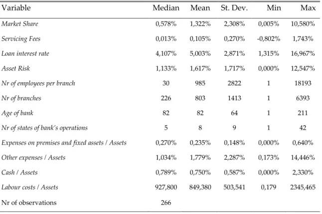
3.4. Summary Statistics
Table I presents summary statistics for all the variables used. The median bank market share is 0,587%, which charges a median service fee of 0,013% which is equivalent to an increase in the loan interest rate of 0,013 pp, and a median interest rate on loans of 4,107%. In terms of characteristics, the median bank has
34
an asset risk of 1,133%, has 30 employees per branch, 226 branches, started operating 82 years ago and has physical presence in 5 states.
Variable Median Mean St. Dev. Min Max
Market Share 0,578% 1,322% 2,308% 0,005% 10,580%
Servicing Fees 0,013% 0,105% 0,270% -0,802% 1,743%
Loan interest rate 4,107% 5,003% 2,871% 1,315% 16,967%
Asset Risk 1,133% 1,617% 1,717% 0,000% 12,547%
Nr of employees per branch 30 985 2822 1 18193
Nr of branches 226 803 1413 1 6393
Age of bank 82 82 64 1 211
Nr of states of bank’s operations 5 8 9 1 42
Expenses on premises and fixed assets / Assets 0,270% 0,235% 0,148% 0,000% 0,640%
Other expenses / Assets 1,034% 1,779% 2,287% 0,173% 14,446%
Cash / Assets 0,789% 0,750% 0,587% 0,000% 2,330%
Labour costs / Assets 927,800 849,380 503,541 0,179 2345,465
Nr of observations 266
Table I – Summary Statistics
4. Estimation Results
Table II presents the estimation results for three specifications of our demand model. The first specification, presented in column (i), denotes the standard multinomial logit demand model, estimated by ordinary least squares. The second specification, presented in column (ii), denotes the same demand model, estimated by instrumental variables. The third and final specification, presented in column (iii), denotes the nested multinomial logit demand model, estimated by instrumental variables. All specifications include the price variables and the
set of observed characteristics discussed above as well as year and bank fixed effects.
The results for the first specification suggest that consumers respond negative and significantly to the service fees, however, the loan interest rate is not significant and, therefore, states that consumers are not influenced by this price variable when choosing a bank, which is not expected and unrealistic. This means that if the service fees increase, the mean utility of the bank in the loan service market will decrease. This result is consistent with what one would theoretically expect. Further, the results also suggest that consumers value negative and significantly the loan portfolio quality of the bank, as measured by its asset risk. Finally, the results also suggest that consumers value positive and significantly the number of branches a bank has available for them to purchase their services and the bank’s age, which may be related to the bank’s perceived experience and expertise, but respond negative and significantly to the number of states in which the bank has presence. All remaining bank characteristics are not statistically significant, suggesting that they do not impact the consumers decision-making process.
However, the ordinary least squares estimates are likely biased due to the potential endogeneity of the price variables, since those variables are presumably correlated with the valuation for the unobserved bank characteristics. The estimation results for the second specification, based on both cost shifters and on BLP instruments, indicate that service fees and loan interest rates continue to be highly significant and to have the expected sign. Further, the results also suggest that asset risk is now not statistically significant. Moreover, the results also suggest that consumers value positive and significantly the number of branches and the number of employees per branch. Finally, the results also report that
36
consumers value significantly the bank’s age, preferring more recent banks. This might be reasonable if we consider that more recent banks are typically more technology-driven, which, considering the current environment, may constitute a preferable attribute. All remaining bank characteristics are not statistically significant, suggesting that they do not impact the consumers decision-making process. I interpret the difference in the estimates obtained when using ordinary least squares (in column (i)) and instrumental variables (in column (ii)) as indicative that correcting for price endogeneity matters.
The standard multinomial logit demand model assumes unreasonable substitution patterns. To account for this problem, the third specification estimates a nested multinomial logit demand model, more flexible than the standard model. As discussed above, in order to estimate the nested model, I have to define a priori the groups of the banks in the market. To do so, the number of states in which the bank has presence is now dropped as an observed characteristic and is now used to nest the banks into two groups: the ones that operate in more than one state and the ones that operate in exactly one state. The estimation results for the third specification, based on both cost shifters and on BLP instruments, indicate that service fees and loan interest rates remain highly significant and have the expected sign. Further, the results also suggest that asset risk remains not statistically significant. Moreover, the results also suggest consumers value significantly the bank’s age, preferring again more recent banks. All remaining bank characteristics are not statistically significant, suggesting that they do not impact the consumers decision-making process. Finally, the results suggest that the true value of 𝜎 ranges from 0,75 to 0,82, which
I interpret as indicative that the nested logit demand model is consistent with consumer utility maximization.7
OLS IV
Explanatory variables (i)
LOGIT (ii) LOGIT (iii) NESTED Service fees -61,319** -294,720*** -75,756*** (24,612) (85,252) (12,337)
Loan interest rate -9,993* -149,218*** -30,147***
(5,606) (29,935) (5,803)
Asset Risk -13,546** 1,374 -3,363
(4,919) (10,123) (3,453)
Nr of employees per branch <0,001* <0,001** <0,001
(<0,001) (<0,001) (<0,001)
Nr of branches 0,004*** 0,002*** 0,0004*
(0,001) (0,001) (<0,001)
Bank’s age 0,057*** -0,247*** -0,036***
(0,011) (0,064) (0,011)
Nr of states of bank’s operations -0,559*** -0,067
(0,145) (0,096)
𝑙𝑛 (𝑠𝑗|𝑔) 0,786***
(0,020)
R-squared 0.913
First-stage R-Sq. (Service fees) 0,982 0,709
First-stage R-Sq. (Loan int. rate) 0,705 0,983
Bank and Year Fixed-Effects YES YES YES
Table II – Demand Estimation Results
Estimated standard errors, robust and clustered by years are in parentheses. Year and bank fixed effects are included in all models.
*significant at 10%; **significant at 5%; ***significant at 1%.
7 I also estimated the nested logit model using bank size as groups, as seen in Dick (2008). The bank size was
determined by the amount of assets a bank owned. However, regardless of price variables, none of the variables was significant. Therefore, I chose to use the number of states in which a bank operates as nests. The results are
38
4.1. Literature Comparison
Molnár, et al. (2006) and Nakane, et al. (2006) are, to the best of my knowledge, the only two examples in the literature that estimate demand for loan services.
Molnár et al. (2006)’s results differ substantially from mine. The number of branches and the number of employees per branch are reported to have a positive and significant impact on demand for loans, whereas the bank’s age is reported to have a positive and significant impact in some type of loans, such as higher purchase and personal loans, but has an insignificant impact on other types such as overdrafts. Contrarily, my results suggest that, except for the the price variables and the bank’s age, neither of the other characteristics has an impact on the decision-making process. Concerning the bank’s age characteristic, my results state that it has a significant and negative impact on loans, whereas they report that it has a positive and significant impact.
Nakane et al. (2006)’s results also differ slightly from mine. The number of states in which the bank has presence is reported to have a negative and significant influence on demand, whereas the branch density and bank’s age are reported to have a positive and significant impact on demand for loans. Which contrasts with my results, since I report that the bank’s age has a negative and significant impact on the demand for loans, and that the other characteristics do not impact demand.
4.2. Asset Risk
The main research question of this thesis is to examine whether the loan portfolio quality of a bank impacts the decision-making process of consumers when purchasing loan services. Lending is the primary source of revenue for banks and, therefore, it is natural that, on one hand, banks may take too much
risk and, on the other hand, regulators intend to discourage the amount of risk that banks take. In the case of deposit services, the answer would be relatively straightforward, although there are deposit insurances provided by the FDIC, consumers would typically prefer more secure and sound banks. However, in the case of loan services, the answer is not so straightforward. On one hand, consumers may believe that if a bank has a riskier loan portfolio, they will more easily approve them a loan. On the other hand, it might not be a good sign of the bank’s health and, therefore, consumers may prefer to choose a less taking-risk bank. This constitutes an empirical question. The results for my preferred specification, the third specification, seem to suggest that the first effect dominates the second, with consumers being estimated not to react to asset risk when choosing loan services.
4.3. Price elasticities
Table III presents the distribution of own-price elasticities for service fees and loan interest rates, computed using the estimates for my preferred specification. For this specification, the own-price elasticity of bank j in year t, are given by:
𝜀𝑗𝑗𝑡𝑓 = 𝛼𝑓𝑝𝑗𝑡𝑓 [𝑠𝑗𝑡∗ − 1 1 − 𝜎+ 𝜎 1 − 𝜎𝑠𝑗𝑡|𝑔 ∗ ] (25) 𝜀𝑗𝑗𝑡𝑟 = 𝛼𝑟𝑝 𝑗𝑡𝑟 [𝑠𝑗𝑡∗ − 1 1 − 𝜎+ 𝜎 1 − 𝜎𝑠𝑗𝑡|𝑔 ∗ ] (26)
The median own-price elasticity associated to loan interest rates is -5,7, whereas the median own-price elasticity associated to service fees is -0,04. The former suggest that banks do not have high market power when setting interest rates. If the bank raised the interest rate by 1%, the demand for loans services would decrease by 5,7%. The latter is, in absolute terms, smaller than one, which
40
suggests that banks have high market power when setting service fees and are clearly not profit maximizing. If the bank raised service fees by 1%, the demand for loans would only decrease by 0,04%. The question is: why do banks choose not to raise service fees until they reach the elastic portion of the demand curve? Dick (2008) argues that there are many explanations for this phenomenon. One of the arguments is that banks may choose to have service fees close to zero since it is a way of attracting and locking-in consumers that will later on purchase more services.
Variable 10% 25% Median 75% 90%
Loan interest rate -12,44453 -7,638501 -5,69596 -4,799161 -3,471927
Service fees -0,85410 -0,38170 -0,04133 0,00000 0,00000
Table III – Price Elasticities
5. Conclusion
This paper estimates the demand for loan services in the U.S. banking industry using a nested multinomial logit demand model, estimated using two types of instrumental variables: cost shifters and BLP instruments. The results seem to suggest that consumers respond negative and significantly to loan interest rates, service fees, and to the banks’ age. The results also seem to suggest that consumers do not significantly respond to asset risk, the number of employees per branch, and the number of branches.
The estimated substitution patterns seem to suggest that banks enjoy high market power when setting service fees, since the median own-service fees elasticity is -0,04, which in absolute terms is smaller than one and therefore
indicates that banks are not profit maximizing. The estimated substitution patterns seem also to suggest that banks do not enjoy high market power when setting loan interest rates, since the median own-interest rate elasticity is -5,7.
This thesis leaves many unanswered questions, which could be addressed using my framework. First, if data becomes available, it would be interesting to examine the determinants of bank lending in other financial institutions (and not only in commercial banks). Second, asset risk may be an important determinant of deposit services, since consumers might be more conscious when choosing where to allocate their deposits, in particular within uninsured depositary institutions.
42
Bibliography
Berry, S. 1994. Estimating discrete-choice models of product differentiation. The RAND Journal of Economics, 25: 242-262.
Berry, S., Levinsohn, J., & Pakes, A. 1995. Automobile prices in market equilibrium. Econometrica, 63: 841-890.
Brito, D., Pereira, P., & Ribeiro, T. 2008. Merger analysis in the banking industry: the mortgage loans and the short term corporate credit markets. citeseerx.ist.psu.edu.
http://citeseerx.ist.psu.edu/viewdoc/download?doi=10.1.1.606.7794&rep=rep 1&type=pdf, September 16.
Cardell, N. S. 1997. Variance components structures for the extreme-value and logistic distributions with application to models of heterogeneity. Econometric Theory, 13(02): 185-213.
Dick, A. 2008. Demand estimation and consumer welfare in the banking industry. Journal of Banking & Finance, 32(8): 1661-1676.
Gorman, W. M. 1956. A possible procedure for analysing quality differentials in the eggs market. Review of Economic Studies, 47: 843-856.
Hausman, J. A. 1996. Valuation of new goods under perfect and imperfect competition. In The economics of new goods: 207-248. Chicago, IL: University of Chicago Press.
Hausman, J., Leonard, G., & Zona, J. D. 1994. Competitive analysis with differenciated products. Annales d'Economie et de Statistique, 34: 159-180.
Lancaster, K. J. 1966. A new approach to consumer theory. Journal of Political Economy, 74(2): 132-157.
McFadden, D. 1981. Structural Discrete Probability Models Derived from Theories of Choice. In C. Manski and D. McFadden (Eds.), Structural analysis of discrete data with econometric applications: 198-272. Cambridge, MA: MIT Press.
McFadden, D. 1973. Conditional logit analysis of qualitative choice behaviour. In P. Zarembka (Ed.), Frontiers of Econometrics: 105-142. New York, NY: Academic Press.
McFadden, D. 1978. Modelling the choice of residential location. In A. Karlqvist, L. Lundqvist, F. Snickars, and J. Weibull (Eds.) Spatial interaction theory and planning models: 75-96. North Holland: Amsterdam.
Meeker, L.G. & Gray, L. 1987. A note on non-performing loans as an indicator of asset quality. Journal of Banking and Finance, 11: 161-168.
44
Molnar, J., Nagy, M., & Horvath, C. 2006. A structural empirical analysis of retail banking competition: the case of Hungary. Available at SSRN 961776.
Nakane, M. I., Alencar, L. S., & Kanczuk, F. 2006. Demand for bank services and market power in Brazilian banking. Working Paper No. 107, Central Bank of Brazil, Brazil.
Shrieves, R. E., & Dahl, D. (1992). The relationship between risk and capital in commercial banks. Journal of Banking & Finance, 16(2): 439-457.