Tesla Inc. : an equity valuation

(1)

Tesla Inc.

An Equity

Valuation

Julie Catarino

152416031

Dissertation written under the supervision of José Carlos Tudela Matins

Dissertation submitted in partial fulfilment of requirements for the MSc in Finance, at the Universidade Católica Portuguesa, 5 April 2019.

(2)

Tesla Inc., An Equity Valuation

By Julie Catarino

Abstract

The purpose of this dissertation is to determine the value of one Tesla, Inc. share as of 31 December 2018. An analysis of the automotive and energy generation and storage industry is presented, together with a detailed analysis of Tesla’s business and financial performance. For Tesla’s valuation purposes, the financial items are forecasted for a period of 10 years, i.e. from 2018 to 2027. In order to determine Tesla’s value, it is used the DCF approach, with the WACC as the discount rate. Additionally, the multiples method is also prepared as a complementary valuation to DCF.

Based on the DCF approach, the achieved Tesla’s price target is $229.95, with a downside of 27.62% when comparing to the actual market share price $317.69, on 31 December 2018. Therefore, it is considered that Tesla is overvalued.

In addition, a sensitivity analysis was completed to variations on WACC, terminal growth rate and total operating costs.

Finally, the estimated Tesla’s share price is compared to the valuation done by J.P.Morgan, which recommended price target is $216 on 31 December 2018. To conclude, both valuations yield to a sell recommendation.

Keywords: Tesla, Automotive Industry, Renewable Energy Industry, Equity Valuation, Firm

(3)

Tesla Inc., Uma Avaliação da Empresa

Por Julie Catarino

Resumo

O objetivo da presente dissertação é determinar o valor de uma ação da Tesla, Inc. a 31 de dezembro de 2018. É apresentada uma análise da indústria automóvel, produção e armazenamento de energia, juntamente com uma análise detalhada do negócio e do desempenho financeiro da Tesla.

Para fins de avaliação da Tesla, são efetuadas previsões das contas financeiras para um período 10 anos, i.e., de 2018 a 2027. Por forma a determinar o valor da Tesla é usado o método DCF com WACC como a taxa de desconto. Adicionalmente, também é usado o método dos múltiplos, como um método de avaliação complementar do DCF.

Com base no modelo DCF, o preço target estimado da Tesla é $229.95, o qual representa um valor de 27.62% abaixo do preço de mercado da ação $317.69, a 31 de dezembro de 2018. Neste sentido, considera-se que a Tesla está sobrevalorizada.

Adicionalmente, uma análise de sensibilidade é efetuada relativamente às variações na taxa WACC, na taxa de crescimento a longo prazo e nos custos operacionais.

Por fim, o preço estimado da Tesla é comparado com a avaliação feita pela J.P.Morgan, que recomendou um preço target de $216 a 31 de dezembro de 2018. Concluindo, ambas as avaliações recomendam uma decisão de venda.

Palavras-Chave: Tesla, Indústria Automóvel, Indústria das Energias Renováveis, Avaliação

do Capital Próprio, Avaliação da Empresa, Fluxo de Caixa Descontados, Avaliação por Múltiplos, Análise de Sensibilidade.

(4)

Acknowledgements

After so many years of study, I am glad to finish my MSc dissertation at CATÓLICA-LISBON. All the courses I took in my Bachelor’s degree in Management and during the Master in Finance were crucial to acquire knowledge and experience in order to complete this dissertation. Firstly, a big thank you goes to my advisor Professor José Tudela Martins for his guidance and availability to help me to accomplish this dissertation.

Secondly, I would like to thank J.P.Morgan’s analyst for providing me with an equity research report on Tesla, which allowed me to complete a chapter of this dissertation.

Thirdly, a special thanks to my parents for giving me the opportunity to pursue this academic path and to my family in general who have supported me during the dissertation journey, which had ups and downs. Thanks to my pets for keeping me company in the late nights after work. Last but not least, I would like to accredit an enormous thank you for all my kind friends who have always motivated me to finish my dissertation. To Joana C., Joana F., and Rosário D., I express my gratitude for all the times they asked me if I was working on my dissertation, for their unconditional support and motivation whenever I need the most.

(5)

List of Figures

Figure 1: Valuation Models ... 12

Figure 2: Valuation Multiples ... 20

Figure 3: World GDP and vehicles sales growth ... 22

Figure 4: Number of electric vehicles from 2013 to 2017 (in millions) ... 22

Figure 5: World energy consumption from 1990 to 2040 ... 23

Figure 6: Annual market size of energy storage in the US (in $millions) ... 24

Figure 7: Renewables’ electricity generation by source from 2015 to 2017 (in TWh) ... 24

Figure 8: % Revenues by business segment in 2017 ... 25

Figure 9: % Revenues by geographic area in 2017 ... 26

Figure 10: Tesla share price development and S&P500 ... 29

(9)

List of Tables

Table 1: Tesla production and deliveries in units by model and CAGR ... 31

Table 2: Model S average sale price and its margin in 2013 and 2014 ... 32

Table 3: Average sale price of Model S, X and 3 in 2019 ... 32

Table 4: Automotive revenue by model from 2013 to 2027 (dollars in millions) ... 33

Table 5: Automotive leasing revenue from 2014 to 2027 (dollars in millions) ... 33

Table 6: Energy generation and storage revenue between 2014 and 2027 (dollars in millions) ... 35

Table 7: Services and other revenue from 2013 to 2027 (dollars in millions) ... 35

Table 8: Cost of revenue between 2013 and 2027 (dollars in millions) ... 37

Table 9: Operating expenses between 2013 and 2027 (dollars in millions) ... 37

Table 10: Net interest expenses from 2013 to 2027 (dollars in millions) ... 38

Table 11: FCFF estimated from 2018 to 2027 (dollars in millions) ... 40

Table 12: WAAC calculation ... 42

Table 13: DCF method – Tesla valuation ... 43

Table 14: Tesla’s peer group selection ... 45

Table 15: Tesla's price per share based on Peers ... 46

Table 16: Sensitivity analysis to terminal growth rate and WACC (share price in dollars) .... 47

Table 17: Sensitivity analysis to total operating costs (share price in dollars) ... 47

Table 18: Comparison with the investment bank valuation ... 48

(10)

1. Introduction

The automotive industry is witnessing a major transformation from the production of only conventional gasoline-powered vehicles to electric vehicles as well. Tesla, Inc does not fit in any traditional model and, in fact, nowadays, is the only car brand that sells only fully electric vehicles. The company has created an impact on the automotive sector. Some years ago, Tesla was the only car manufacturer that produced and sold fully electric vehicles, however, currently, several established companies are offering this type of car to the market.

Based on the above, the aim of this dissertation is to enlarge the study of Tesla and find its value as of 31 December 2018. Therefore, the research question is defined as follows:

What is the value of one Tesla, Inc. share?

Additionally, one of the main intentions of this dissertation is to infer whether Tesla’s value is overvalued as commonly said between analysts.

For that purpose, a valuation overview and the most well-known and used valuations methods will be presented in the literature review chapter. Afterwards, an analysis of the industry and of the Company will be described, in order to understand the industry, the past and the potential future performance of Tesla.

Then, the dissertation will move on to a detailed forecast of Tesla’s financial items, accompanied by the computation of Tesla’s value, based on the DCF and Multiples method. In the following chapter, a sensitivity analysis is performed to determine the impact of the change of a key assumption on Tesla’s valuation.

In the end, the valuation of Tesla will be compared with the valuation performed by the investment bank J.P.Morgan, and the stock recommendation decisions will be identified.

(11)

2. Literature Review

The aim of this chapter is to give a general understanding of the most well-known valuation approaches before presenting the equity valuation performed on Tesla. This chapter starts with a valuation overview.

Afterwards, the DCF approach and Relative valuation are described. Other relevant valuation methods, namely the Adjusted Present Value (APV), Dividend Discount Model (DDM) and Economic Value Added (EVA), are described in Appendix 1. For each valuation approach described in this section, it is explained their main assumptions, in what conditions the method is more suitable to be used and some limitations.

Finally, this chapter will close with defining the valuation methods used to value one share of Tesla.

2.1. Valuation Overview

Over the past years, the importance of valuation has been increasing. The knowledge of the mechanism of enterprise valuation has become a prerequisite for enterprise’s resource-allocation decision, as it identifies the value of each decision (Luherman, 1997). As a matter of fact, the process of valuing an enterprise and its business units enables to identify sources of economic value creation and destruction within the enterprise (Fernández, 2007). Therefore, companies take advantage of this knowledge to make wiser strategic and operating decisions, such as what businesses to own and how to make trade-offs between growth and returns on invested capital (Koller, Goedhart, & Wessels, 2015).

Damodaran (2002) claims that information related to a specific enterprise may affect an entire sector or expectations for all enterprises in the market. As a result, the majority agrees that when valuing an enterprise, a detailed analysis of the enterprise should be done, regarding market position, investment policy, profitability, finance structure, management characteristics and quality of human capital, as well as, an analysis of the industry, competitors, economic environment, macroeconomic and politics.

However, regardless of how deep the analysis can be, there will always be uncertainty about the final enterprise value reached as assumptions concerning the enterprise and economy future are made throughout the valuation (Damodaran, 2002). Additionally, Fernàdez (2004) explains

(12)

that the most common and uncommon errors in enterprise valuation are related to discount rate calculations, valuing the enterprise riskiness, forecasting cash flows, residual value, among others.

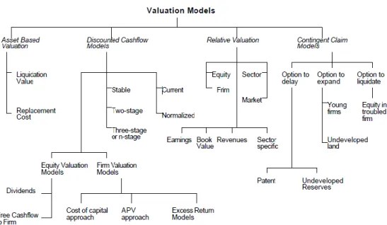
Currently, there are several approaches to valuation (figure 1). According to Young, Sullivan, Nokhasteh, & Holt (1999, p.4), “most popular valuation approaches are different ways of expressing the same underlying model” and, therefore, as the authors show in their paper, these referred approaches are mathematically equivalent under certain assumptions.

Although over the years there were several valuation frameworks studied and implemented, there is no single framework expected to be consistently more reliable than others (Young et al., 1999). According to Damodaran (2006), there are four main approaches to company valuation: Asset Based Valuation, Discounted Cash Flow, Relative Valuation and Contingent Claim Valuation, as shown in figure 1.

Figure 1: Valuation Models

Source: Damodaran, 2002, Chapter 35 p.3

In general, the younger the company is, the more difficult is the company valuation, because of the lack of historical data and uncertainty about fundamental factors and their forecasts (Festel, Wuermseher & Cattaneo, 2013). According to Damodaran (2011), younger companies are more difficult to value because are dependent upon future growths, are more exposed to failure and there is uncertainty about when the company will become a stable growth company.

(13)

relative valuation such as price earnings ratios are not applicable. Moreover, Petersen and Plenborg (2012) affirm that companies that share these characteristics are not directly comparable with well-established companies, regardless of belonging to the same industry.

2.2. Discounted Cash Flow Valuation

Koller et al. (2015, p.313) state that the Discounted Cash Flow (DCF) model is the “most accurate and flexible method for valuing projects, divisions, and companies”. However, the author highlights the risk of making mistakes due to errors in estimating relevant components used for valuing a company, as there is a large number of assumptions and projections made throughout the valuation.

Also, Gup and Thomas (2010) suggest that this referred model is the most sophisticated because it is based on cash flows resulting from the balance sheet statement and the income statement, takes into consideration the opportunity cost of capital and, finally, it reflects the period in which the cash flows are explicitly forecast.

On the contrary, Luehrman (1997) pointed out that the DCF model that uses the weighted average cost of capital (WAAC) approach is obsolete. Additionally, the author states that the WAAC approach is still used just because is seen as standard over the years and not because it performs the best.

The DCF approach determines the asset value by forecasting the future cash flow of an asset, discounting it at an appropriate rate (r) that reflects the risk of that asset (Damodaran, 2006; Luehrman, 1997). Indeed, the enterprise is worth for its capacity to generate value and, the enterprise value arises mainly from the capacity to generate future cash flows. The general formula of the DCF approach is the following equation (Fernández, 2007):

Asset′_{s Value =} CF1 (1 + r)+ CF₂ (1 + r)2+ CF₂ (1 + r)3+ ⋯ + CF_n+RV_n (1 + r)n RV = CFn(1 + g) (r − g)

In the DCF approach, the cash flows (CF) are forecasted under numerous assumptions about how the company will perform during the explicit period and by forecasting financials items related to the company’s operation, which are responsible for cash flow creation (Fernández, 2007). According to analyst, the explicit period of forecasts is commonly 5 or 10 years,

(14)

depending on when a company enters into a stable growth stage. The above formula is also composed by the residual value (RV), usually called as terminal value (TV), where it is assumed a cash flow with a specific constant growth rate (g) after year n. Young et al. (1999) affirm that the TV is the most important element in a company’s valuation.

There are two approaches to use cash flow for valuation, namely, Free Cash Flow to Equity (FCFE) approach and the Free Cash Flow to the Firm (FCFF).

FCFE

According to Fernández (2007, p.16), the FCFE is the “cash flow remaining available in the company after covering fixed asset investments and working capital requirements and after paying the financial charges and repaying the corresponding part of the debt’s principal (in the event that there exists debt)”. Therefore, the succeeding equation determines the FCFE: FCFE = FCFF − Interest Expenses ∗ (1 − tax rate) − Pincipal Repayments +

Net Debt Issues

FCFF

Fernández (2007, p.14) defines the FCFF as being the “cash flow generated by operations, without taking into account borrowing (financial debt), after tax”. Furthermore, it is the cash flow available to the company after considering the operation expenses, fixed asset investment and working capital investments. The general equaition of FCFF can be written as follows (Damodaran, 2006):

FCFF = EBIT ∗ (1 − tax rate) + Depreciations − Capital Expenditure − ΔWorking Capital In contrast to FCFE, which cash flows are after interest payments and debt cash flows, the cash flow demonstrated on the equation above, are before debt payments and after taxes and reinvestment needs (Damodaran, 2006). Therefore, tax benefits of debt are not included on FCFF. However, the discount rate, WAAC, incorporates this benefit as it uses the after-tax cost of debt (Damodaran, 2002).

The enterprise value can be determined as the present value of the projected FCFF and of the TV, discounted at WACC, as shown on the following equation (Damodaran (2006):

(15)

The main difference between FCFF and FCFE arise primarily from cash flows used as starting point, cash flow from operations or cash flows for shareholders, respectively, as well as cash flows associated with debt (Damodaran, 2002).

2.2.1. Terminal value

The terminal value is the company’s expected cash flows value beyond the explicit period (Mauboussin, 2006). Damodaran (2009) states that the TV represents a large proportion of the enterprise value, and it is even larger when it is concerned a young company. Young et al. (1999) affirm that the TV is the most important element in a company’s valuation.

The TV assumes that cash flows, discount rate and growth are constants over time (Young et al., 1999). As a result, assumptions about when a company will reach a steady stage and with what growth rate may have a huge impact on the enterprise value Mauboussin (2006). Therefore, terminal value should be determined when the company has achieved “low revenues growth and stable operating margins” (Koller et al., 2015, p.216).

The following equation is commonly referred by authors in order to determine the TV:

Terminal Value = FCFFn(1 + g) (WAAC − g)

Although capital expenditures may be lower than depreciations, the TV should not be estimated with capital expenditures lower than depreciations, as it is not consistent to use a FCF with these values (Fernández, 2004). Furthermore, the expected growth rate should be lower than the economy growth rate (Koller et al., 2015).

2.2.2. Weighted Average Cost of Capital

The WAAC, also known as cost of capital, is defined by Young et al. (1999, p.14) as the “after tax cost of debt multiplied by the proportion of debt plus the cost of equity multiplied by the proportion of equity”: WACC = Rd∗ (1 − T) ∗ D V+ Re∗ E V

WACC reflects equity and debt investors’ expected return for the time value of money and the risk related to an asset (Petersen & Plenborg, 2012). In case of default, debt holders have the

(16)

priority and, therefore, cost of debt should be lower than the cost of equity. Consequently. the required rate of return must be calculated separately for the two-types of investors.

According to Damodaran (2006), the cost of capital should reflect only the company’s operating risk, as the cash flows used are cash flows from the operating assets. The free cash flow is determined in after-tax term, therefore, WACC should be estimated after corporate taxes (Koller et al., 2010).

Although there are many valuations that use the marginal tax rate, Fernández (2004) affirms that the tax rate that should be used to calculate the WAAC is the effective tax rate. On the contrary, Pinto et al. (2010, p.77) defend that “cost of capital based on the marginal tax rate usually better reflects a company’s future costs in raising funds” and, also, the effective tax rate may reflect nonrecurring items.

2.2.3. Cost of Debt

Cost of debt represents the effective cost that a company has to pay for its current debt (Damodaran, 2002). Damodaran (2002) explains that the cost of debt is estimated by three variables. First, the riskless rate, which increases the cost of borrowing money, as that rate increases. Second, the company’s default risk, that is, the probability of a company defaulting. Likewise, as the default risk increases, the cost of debt shall also increase. Last, the tax benefit arising from the contracted debt and paying interest, which allows the after-tax cost to be lower than the pre-tax cost of debt. Damodaran (2002, p.39) states that “since interest is tax deductible, the after-tax cost of debt is a function of the tax rate”.

Therefore, the cost of debt should be calculated on an after-tax basis, as regards companies without tax exemption with market values rather than book values:

After tax cost of debt = Pre − tax cost of debt ∗ (1 − tax rate)

Regarding publicly traded companies, Koller et al. (2010) suggest to calculate the Yield to Maturity (YTM) from the bond’s price and promised cash flows, to calculate the cost of capital. However, most of the companies do not trade on a regular basis and, therefore, one should estimate a default spread based on the company’s debt rating (Damodaran, 2002).

(17)

Interest coverage ration = EBIT Interest Expenses

Damodaran (2002) affirm that with this computation it is possible to associate to a company rating and, therefore, to obtain a default spread (appendix 16). Consequently, the cost of debt can be estimated by:

Cost of debt = Risk − free rate + default spread

2.2.4. Cost of Equity

Over the past years, the capital asset pricing model (CAPM) developed by Sharpe (1964) and Lintner (1965) and, built on the model of portfolio choice presented by Markowitz (1959), is still the most commonly accepted asset pricing model and widely used for calculating the cost of capital.

The cost of equity is the rate of return investors require on an equity investment in a firm (Damodaran. 2002). In order to calculate the cost of equity (expected return (E(R)), it must be estimated the risk-free rate of return (Rf), the difference between the expected return on a market portfolio (Rm) and the Rf, defined as the market risk premium and, the market risk of a particular asset (β) (Koller et al., 2010). Therefore, based on CAPM, the general equation to estimate the cost of equity is the following:

E(R) = Rf + β [E(Rm) − 𝑅𝑓]

Fama and French (2004, p.25) believe that the CAPM is commonly used in applications because it “offers powerful and intuitively pleasing predictions about how to measure risk and the relation between expected return and risk”. However, CAPM can reveal weaknesses in the theory or in its empirical implementation, thus making the majority analysis done with the referred model invalid. Despite recent critiques, when developing a company valuation based on WACC, the CAPM remains to be the most used model for estimating the cost of equity.

2.2.5. Risk-free rate

Fernández (2004) defines the risk-free rate as the rate that can be obtained at the time when the cost of equity is determined by using risk-free government bonds at the same time.

According to Damodaran (2009, p.165) a rate to be considered as risk-free needs to meet two conditions: “first that no risk of default is associated with its cash flows and second that there can be no reinvestment risk in the investment”.

(18)

Most empirical researchers suggest to use the long-term government treasury bonds to calculate the risk-free rate, in developed economies (e.g. 10-year zero coupon governmentbonds). Since government bonds are usually issued with different maturities, it should be used a government default-free bond with the same maturity as the maturity of the discounted cash flows (Koller et al., 2010).

2.2.6. Beta

Zenner et al. (2008, p.1) define beta as a “calibration factor that is higher (lower) that one if the asset has a systematic, or non-diversifiable, risk that is higher (lower) than the market’s risk”. Therefore, beta represents the market risk of a particular asset. Moreover, it is different across companies and varies according to the period that is was calculated (Damodaran, 2001). Koller et al. (2010) state that, according to CAMP, the expected return of a stock depends on beta, which represents the correlation between that stock’s value and the market. The authors suggest estimating beta by using regression.

According to Damodaran (2002), beta can be estimated by using a regression of the historical stock returns of an investment against the historical market, as follows:

R_j = α + β ∗ Rm

The slope of the regression-corresponds to the beta of the stock.

One component needed to calculate the cost of equity is the levered beta (also known as equity beta). The additional risk arising from the fact that the company has debt, in other words, from the leverage, can be expressed as follows:

βL= βU∗ [1 + (1 − T) ∗

D E]

Damodaran (1994) assumes that debt carries no market risk, thus, having a debt beta of zero. Conversely, Fernández (2004, p.5) states that the correct relation between the levered beta (βL)

and the unlevered beta (βU) is:

βL= βU+ (βU− βD)∗

D ∗ (1 − T) E

(19)

2.2.7. Market Risk Premium

The Market Risk Premium (MRP) is defined as the “incremental premium required by investors relative to a risk-free asset” (Zenner et al., 2008, p.1). CAMP proposes an adjustment on the equation commonly used1_{through the adjustment on the MRP with beta:}

Expected Market Portfolio Return = Rf + β ∗ MRP

Additionally, Zenner et al. (2008) propose several methods to estimate MRP, namely, historical average realized return, dividend discount model, constant Sharpe ratio method, bond-market implied risk premium, dividend yield method and Survey evidence. On their paper, they concluded that MRP falls most likely between 5% and 7%.

Koller et al. (2010) classify as the appropriate premium range between 4.5% and 5.5%. Further, Bruner et al. (1998) research indicated that most of the best-practice companies use a MRP of 6% or lower despite the fact that many authors and analysts use higher premiums.

Although the numerous researches done, and papers published, there is no consensus among practitioners regarding the best model to estimate this component.

2.3. Relative Valuation

Relative valuation seeks to estimate the value of a company through the comparison with other companies, which are similar to that company, in other words, the value of an asset is compared to that of another similar or comparable asset (Damodaran, 2002).

Goedhart et al. (2005, p.1) state that “a properly executed multiples analysis can make financial forecasts more accurate”. The authors suggest that the DCF valuation become more accurate as well as their forecasts with a detailed analysis comparing the multiples of the company valued with those of the comparable companies. Similarly, Fernández (2001) states that relative valuation can be useful in a second stage of the valuation, by reviewing the completed valuation and multiples, as well as, by carefully identifying differences between the company that is being analysed and the comparable companies.

(20)

As per Goehart et al. (2005), analysts should not use industry average because companies in the same industry as the company valued may have significantly different growth rates, return on invested capital (ROIC) and capital structures.

According to Goehart et al. (2005), there are four basic principles in order to properly value a company based on multiples. It is essential to find a peer group and use peers with similar ROIC and growth forecasts. Besides that, another basic principle is the use of forward-looking multiples. As a matter of fact, both the principles of valuation and the empirical evidence suggest that forward-looking method should be followed as it is more accurate than historical multiples (Goehart et al., 2005 and Koller et. al., 2010). Finally, the use enterprise-value multiple, as well as the adjustment of this multiple for nonoperating items also represent a basic principle.

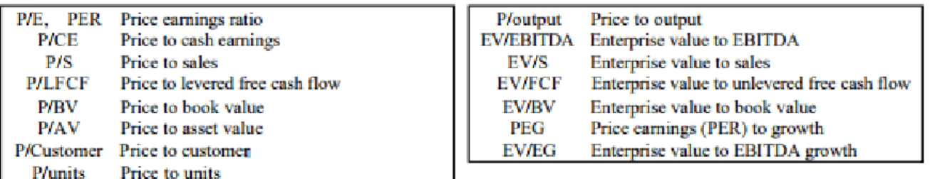
According to Fernandez (2001), the most commonly used price and enterprise value multiples are the following:

Figure 2: Valuation Multiples

Source: Fernandez 2001, p.3

Damodaran (2002) reveals that almost 90% of equity research valuations use relative valuations. In fact, according to Lie and Lie (2002), valuations performed with multiples are often preferred rather than with DCF approach, since it is difficult to estimate cash flows and to find the adequate discount rate. Besides, multiples are simple and easy to work with (Damodaran, 2002).

According to Damodaran (2006, p.650), a comparable company is “one with cash flows, growth potential, and risk similar to the firm being valued”. In general, comparable companies belong to the same sector. However, this approach becomes harder when there are not enough companies in the same industry which share similar cash flows, growth and risk profiles (Damodaran, 2006). Goedhart et al. (2005) explain that in order to obtain the right companies, those have to have similar expectations regarding long-term growth and ROIC.

(21)

Overall, when choosing the peer group there are several components that should be analysed, such as, business area, size, growth, debt to equity and profitability. However, it is often difficult to find a true peer group.

According to Koller et al., (2010) enterprise value to EBITDA is wildly used and perceived as the best multiples for comparing valuations across companies. Price-to-Earnings (P/E) cannot be calculated for companies with zero or negative earnings (Pinto et al., 2010). About EV-to-Sales multiple, this multiple is useful for companies with “volatile earnings volatile earnings or other situations when earnings fail to represent long-term operating potential” (Koller et al., 2010, p.327).

Conclusion

In this thesis, the valuation methods used to value one share of Tesla are the DCF and Multiples method. The DCF approach was chosen as it is widely used on equity valuations and for its accuracy and flexibility. Although the DCF model does not discriminate the tax shields advantages or the distress costs, it provides a more complete analysis regarding the company’s operations. Lastly, Multiples method are used as a second stage of Tesla equity valuation in order to verify the DCF results and to compare with its peer group.

(22)

3. Industry Overview

The automotive industry has been growing, at least, from the last 8 years (figure 3). Over the years, more and more cars are sold worldwide. Due to a growing economy, environmental consciousness, increase of oil prices and government incentives to electric cars, the automotive industry is witnessing a major transformation – the development of battery electric (BEVs) and plug-in hybrid electric (PHEVs) vehicles. However, conventional cars are expected to continue to dominate in the coming years.

Figure 3: World GDP and vehicles sales growth

Source: World Bank, OICA and own calculations

Nowadays, most automakers are producing and developing fully electric cars (EVs) and consumers are becoming more open-minded to this type of cars. In 2017, more than 3 million electric vehicles were sold worldwide, a growth beyond 55% from the previous year (figure 4). From 2016 to 2017, sales of EVs rose 90%, 36% and 57% in China, in the US and in Europe, respectively.

Figure 4: Number of electric vehicles from 2013 to 2017 (in millions)

-10% -5% 0% 5% 10% 15% 2006 2007 2008 2009 2010 2011 2012 2013 2014 2015 2016 2017 World GDP World vehicles sales

0,38 0,71 1,23 1,98 3,11 0 0,5 1 1,5 2 2,5 3 3,5 2013 2014 2015 2016 2017 Millio ns

(23)

Despite significant growth in sales, the EVs only stood for 0.2% of the market share in 2017. BEVs and PHEVs sales are expected to rise in market share from 1% in 2017 to 20% in 2030. The demand in China has been significantly increasing in the past years and was the largest market for electric vehicles in 2017, with 1.23 million EVs. In 2017, China represented around 40% of all global EVs sales. In addition, the Chinese government believes that by 2025 7million EVs may be sold per year. Electric vehicle market in the US is expected to grow from 0.83% to 7.08% by 2025 of total cars sales in that country. Concerning Europe, there are more than one million EVs in the European roads and Norway is the leader country with a higher number of electric cars.

Government incentives for the purchase of EVs are becoming more frequent in several countries around the world. This consist of, for instance, tax exemptions on the cars, free tolls and parking, subsidies. In the US, a tax credit of $7.500 is applied on the acquisition of an electric car, if certain conditions are met. Accordingly, these government measures are encouraging the purchase of EVs, which contributes to the constant growth of sales of those cars.

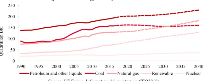
The world consumption of energy has been generally increasing for all fuels over the past years. In addition, the referred consumption is expected to continue to increase, on average, for Petroleum, coal, natural gas, renewable and nuclear (figure 5). Globally, renewable energy is more and more used as a fuel and, it is estimated that, from 2017 to 2040, its consumption will rise by 70%. In addition, renewable energy will account for 17% of all world consumption whereas petroleum and other liquids may account for 31% in 2040.

Figure 5: World energy consumption from 1990 to 2040

Source: US Energy Information Administration (IEO2018)

0 50 100 150 200 250 1990 1995 2000 2005 2010 2015 2020 2025 2030 2035 2040 Qu ad rilli on B tu

(24)

Renewable energy was the source of energy that had the highest growth in 2017 (3.3%). With that increase, the energy storage deployments are increasing as well. According to GTM Research and Energy Storage Association (ESA), energy storage deployments are expected to grow from 2018 to 2019 by 154%, in the US. It is estimated that the market size of energy storage will represent 4,561 million of dollars in 2023 (figure 6). Additionally, this growth is mainly due to the increase in “residential deployments as customers continue to exhibit increased interest in self-consumption and resilience” (GTM Research and ESA, September 2018).

Figure 6: Annual market size of energy storage in the US (in $millions)

Source: GTM Research and ESA

Together with the rise of consumption of renewable energy, the energy generation has been growing in absolute number for all type of sources and, overall, in 2016 and 2017 they saw a rise of 7.3% and 6.9%, respectively (figure 7). The Solar Photovoltaic (Solar PV) was the source that had greater growth, with 32% higher generation in 2017, in relation to the previous year. In fact, the Solar PV may be considered as the most affordable source of electricity generation in many countries.

Figure 7: Renewables’ electricity generation by source from 2015 to 2017 (in TWh)

$4 561 $541 $0 $1 000 $2 000 $3 000 $4 000 $5 000 2023 2018 0 1000 2000 3000 4000 5000 6000 2017 2016 2015 Hydropower Wind Solar PV Other 5,932 5,172 5,549

(25)

4. Tesla Inc. Overview

4.1. Introduction

In 2003, Matin Eberhard and Mar Tapenning founded Tesla, Inc., formerly Tesla Motors, Inc., an American automotive company that designs, develop, manufacture and sells high-end fully electric vehicles as well as powertrain components for electric vehicles. Elon Musk, the current CEO and Co-founder, said in one of his presentations in 2016 that “it is very important to accelerate transition to sustainable transport” and this is the main goal of Tesla.

Nowadays, Tesla is a well-known and recognized worldwide brand. The Company was considered the 4th_{largest automotive company by market value and the largest in the US, in}

early 2017, despite having just sold around 76,000 cars during 2016.

Today, Tesla produces and sells not only electric vehicles but also infinitely scalable clean energy generation and storage products in the US and abroad.Thereby, the Company operates in two segments, the automotive sector and energy generation and storage sector. Tesla operates in the energy sector since 2014, and this stood for 0.13% and 0.36% of the total sales in 2014 and 2015, respectively. During 2017, the first segment represented around 91% of the total revenues and energy generation and storage sector about 9% (figure 8).

Figure 8: % Revenues by business segment in 2017

Currently, the US, China and Norway are the main regions where Tesla’s revenues arise. Figure 9 shows the distribution of total revenue across each geographic area between 2012 and 2017, as well as the total revenues performance in millions of US dollars.

91% 9%

Automotive & Services and Other Segment Energy Generation and Storage Segment

(26)

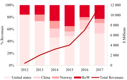
Figure 9: % Revenues by geographic area in 2017

Source: Tesla Annual Report and compiled by the author

In 2013, Tesla expanded its Supercharger network to China, as that country was an important part of Tesla’s growth strategy and was/is perceived to be one of their largest market within a few years.

Along the years, the US continues to play an import role in Tesla’s revenues. In 2017, the US represented about 53% of the total revenues, where China represented around 17% (figure 9). Additionally, Norway, the most significant European country for Tesla, stood for 7% of the total revenues and, the remaining 23%, were distributed in the rest of the world (RoW).

4.2. Automotive Sector

In 2008, Tesla launched the first car, the Tesla Roadster, which was the first fully electric sport car to be sold to the market and costed more than one hundred thousand US dollars. Additionally, at the end of 2012, Tesla stopped the production of this car and sold around 2,450 cars in over 30 countries between 2008 and 2012, mostly in North America and Europe. By 2009, Tesla announced the second model, the Model S, which is considered the first luxury electric car and a prototype was presented in a public exhibition. However, only after 3 years of Model S announcement, the model was available to its customers (in 2012). At the end of that year, Tesla delivered around 2,650 Model S and had 15,000 customer reservations.

0 2 000 4 000 6 000 8 000 10 000 12 000 0% 20% 40% 60% 80% 100% 2012 2013 2014 2015 2016 2017 $ Millio ns % R ev en ues

(27)

to build supercharges through California, in order to enable its customers to make long distant travels. The supercharges are considered as the fasted and most sophisticated charging network in the world. By November 2018, there were 1,375 supercharger stations with 11,414 supercharges around the world.

In early 2013, Tesla was struggling as did not have enough capital to continue Model S production and meet its customer expectations. Furthermore, the Company almost filed for bankruptcy, however, in the first quarter of 2013, Tesla registered profits for the first time since went public and after 10 years of its incorporation.

The goal of Elon Musk with Model 3 is to reach massive production. Only one week after Tesla started to accept pre-orders for Model 3, they received more than 350 thousand pre-orders, which amounts to approximately 14 billion dollars in expected sales. However, the production of this model was delayed and Tesla initial target of production - producing more than five thousand cars per week by the end of 2017 - was not achieved. Consequently, the Company just delivered 1,542 Model 3 cars in 2017. According to Tesla third quarter report, Tesla was producing around 4,300 Model 3 cars per week and delivered 56,065 Model 3. In total, Tesla delivered nearly 70,000 cars in the US in the third quarter. The Company started to accept orders for Model 3 both in Europe and in China during 2018 and will start to deliver it to customers during 2019.

Indeed, Tesla has arranged with Shanghai’s government to allow them to build a Gigafactory 3 in Shanghai, which will be fully owned by Tesla. The EVs market had been increasing significantly in Chine and is by far the largest in the world. Tesla aims to achieve a production of 500,000 vehicles in that factory in 2020/21, which should only meet the Chinese demand. Further to these four models, in November 2017, Tesla unveiled an upcoming semi-trailer fully electric, the Semi Truck. Additionally, in the same presentation, Elon Musk announced the second generation of Roadster as well. The first is expected to be built in full-scale production in 2019 and delivered to customers by 2020. The latter will be the fastest luxury car ever made and should be available in the market also in 2020. However, it is expected that those productions may perhaps be delayed.

(28)

4.3. Energy generation and storage Sector

Another sector where Tesla is operating is the energy generation and storage sector with the aim of creating an entire sustainable energy ecosystem. Tesla Energy was launched in 2015 and is becoming a leader in this sector. Additionally, Tesla acquired SolarCity in November 2016. The Company manufactures and develop energy storage products for homes, commercial use and utilities sites, such as Powerwall, Powerpack and Solar Roof. The first is designed for residential use and was sold for the first time in 2013. This product is an important element for Tesla to achieve the major end goal of energy generation and storage at home. The second product is designed for both commercial and utility sites and was available to customers during 2014. These products generate renewable energy, store it and, afterwards, the energy stored can be consumed. Tesla has been developing a second generation of these systems. The last, Solar Roof, was revealed in 2016 and is conceived to complement and power homes and commercial sites. This solar energy system was installed for the first time in July 2017.

For the Model 3 production of scale and for Tesla energy products, Tesla needs a huge amount of lithium-ion batteries. In fact, Tesla aimed to be able to produce 500 thousand vehicles during 2018 and one million in 2020. This means that to reach these values, the Company would require the entire supply of lithium-ion batteries in the world. Therefore, in 2014, it was announced the plan to construct a giant factory able to produce batteries - the Gigafactory. Nowadays, Gigafactory is already supplying the so-called new generation batteries to cars, houses, companies and some cities. This factory will help to decrease significantly the batteries costs through innovative manufacturing, economies of scale and reduction of waste. The batteries packs’ costs are expected to decrease through the years, as the production of batteries increases. Elon Musk believes that when the Gigafactory will be fully operational by 2020, the price of batteries packs used in its EVs will reduce by 30%. Furthermore, the reduction will allow Tesla to reduce its operational costs in the long-term and reduce its EVs price in the future.

Moreover, one can say that the increasing price of fuel petrol and global warming, as well as the geopolitical factors, may be the reason for Tesla’s long-term survival.

(29)

4.4. Tesla stock market performance

On 29 June 2010, Elon Musk, decided to take Tesla public under the ticker symbol “TSLA” on the Nasdaq Global Select Market, with a total amount of 13,300,000 Initial Public Offer (IPO) shares with a share price of $17. Therefore, the IPO allowed Tesla to raise over $225 million and was the first American automotive company that went public since Ford Motors IPO in 1956. Until today, Tesla is not paying dividends.

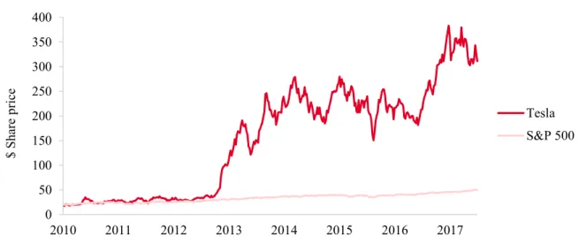
Figure 10 shows Tesla share price development since its IPO and the S&P500 share price development as if on Tesla IPO it would have the same adjusted closed price, i.e., $19.20, then it was considered the same changes of its historical price.

Figure 10: Tesla share price development and S&P500

Source: Thomson Reuters and own calculations

As per the above figure, one shall notice that, up to the beginning of 2013, Tesla share price tracked S&P500 index. However, afterwards, the two-path started to diverge significantly. As a matter of fact, Tesla registered profits for the first time in the first quarter of 2013, since its incorporation. One year later, Tesla’s price had risen by approximately 460%, to $212.37. The stock price achieved a record high of $383, in June 2017.

Although Tesla has been reporting losses of millions of US dollars during the past years, its market capitalization exceeded that of Ford and General Motors in June 2017, corresponding to $60.3, $45.4 and $52.4 billion, respectively. The constant expansion and implemented strategies have made possible for Tesla to exceed the market expectations, which has resulted in a continuous market value increase.

0 50 100 150 200 250 300 350 400 2010 2011 2012 2013 2014 2015 2016 2017 $ Sh ar e pr ice Tesla S&P 500

(30)

5. Tesla Inc. Valuation

An equity valuation is conducted to answer the next question:

What is the value of one Tesla Inc. share?

Both DCF and Relative valuation methods will be used in order to value Tesla’s price per share on 31December 2018.

This chapter will start with the forecasting of financial items from Tesla’s income statement and balance sheet. Further on, the FCFF will be calculated together with the chosen discount rate, WAAC. The succeeding section will concentrate on the calculation of the present value of FCFF and terminal value. All these estimations will consider some assumptions, which are discriminated below. Finally, this chapter will be concluded with a relative valuation.

5.1. Forecasting Income Statement

In this section, several accounting items from the income statement will be forecasted for the next 10 years, i.e. from 2018 to 2027. The financial items’ forecasts are mainly based on the Company’s past performance and assumptions regarding its future performance and of the automotive and energy industry. Nevertheless, a more detailed analysis of those financial items and their forecasts is presented below.

Revenues

Tesla’s total revenues are forecasted by taking into consideration each segment of revenue separately, as follows:

i) Automotive revenue

For the year 2018, only the last quarter of 2018 is necessary to forecast. The automotive revenues of the 2018 fourth quarter wer estimated based on the equivalent quarter of 2017 and the historical growth of the same quarter of the previous year, as follows:

Rev_{fourth quarter2018}= Rev_{fourth quarter2017}∗ (1 + historical growth)

(31)

consequently, the expected number of vehicles delivered and on the average sale price of each model.

Elon Musk aimed to produce 500,000 vehicles during 2018. However, by analysing Tesla’s current situation of its production capacity and past events, it is expected that the production will be higher than 500,000 cars manufactured only by 2023 (appendix 5).

Moreover, it is expected that Tesla will produce higher volumes of Model 3 than Model S and X together. Therefore, it was estimated that the number of Model 3 fabricated will exceed the other models. In addition, Model 3 became the main priority for Tesla, in order to reach mass production and economies of scale in the near future with the purpose of having lower costs of production and higher market share in the EVs market.

It is estimated that that Model S car sales from 2019 to 2023 will follow the same CAGR of the past 3 years, i.e. 4.18%, and then the units sold will growth at the same rate as the forecasted US GDP growth (2%).

Model X was introduced to the market in late 2015. As a result, from 2015 to 2016 the number

of deliveries increased exponentially from 212 to 25,335 (10631%) and from 2016 to 2017 increased by 84% (table 1). Thus, it was estimated that Model X shall increase in percentage more than Model S, with a YoY growth of 10% until the beginning of the steady period (2023). As from 2023, the increase in car deliveries will become more stable and converge to 2% over the steady period.

Table 1: Tesla production and deliveries in units by model and CAGR

2013 2014 2015 2016 2017 1,2,3Q 2018 CAGR

Production _{(without the 4Q 2018)}

Model S 23 187 35 125 50 835 56 022 _{53 092} _{38 793} 23.01% Model X 260 27 900 _{45 250} _{37 599 1219.24%} Model 3 _{2 685} _{91 583} - Total production 23 187 35 125 51 095 83 922 101 027 167 975 Deliveries Model S 22 477 31 655 50 446 50 950 _{54 754} _{37 130} 24.93% Model X 212 25 335 _{46 558} 34 630 1381.94% Model 3 _{1 772} _{82 687} - Total deliveries _{22 477 31 655 50 658 76 285 103 084} _{154 447}

As illustrated in table 1, Tesla ended the year of 2017 producing 2,685 Model 3 and by the end of 2018 third-quarter Tesla reported 82,687 deliveries and a production amounting to 91,583.

(32)

today, Tesla is not able to meet demand due to its production limitations, but this is expected to be diminished with its Gigafactories.

The electric vehicle market is increasing significantly year by year. The global number of EVs sales is expected to grow from 2018 to 2024 at a CAGR of 23.9%, from 9.4 million sales in 2017 to 51.5 million sales in 2024. Additionally, the CAGR of Model S deliveries from 2013 to 2017 corresponds to 24.93% (table 2). As per the above, as from 2019, the Model 3 production was forecasted based on the average of the two mentioned growth rates (24.42%). As from 2023, the growth rate will smoothly decrease over the years to 5%.

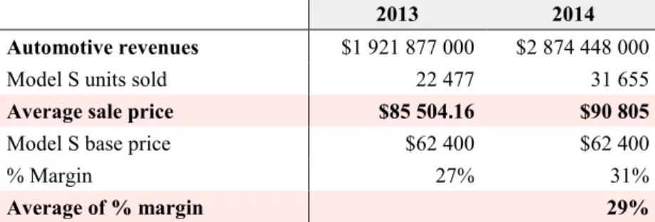
Overall, the main goal of Tesla is to create an EVs priced to compete with its gasoline-powered equivalents and that would be considered the first mass market of EVs in the world. For that reason, in 2027, the Model 3 will account for 87% of automotive revenues (appendix 5). The average sale price was calculated by considering the years 2013 and 2014, as in those years Tesla only sold Model S. By knowing the number of cars sold and its base price in the referred years, the average sale price and its margin was found (table 2).

Table 2: Model S average sale price and its margin in 2013 and 2014

2013 2014

Automotive revenues $1 921 877 000 $2 874 448 000

Model S units sold 22 477 31 655

Average sale price $85 504.16 $90 805

Model S base price $62 400 $62 400

% Margin 27% 31%

Average of % margin 29%

Source: 2013 and 2014 Tesla Annual Reports and own calculations

It is assumed that the average sale price of each model in 2019 will have the same average price margin as the one calculated in table 2, as represented in table 3.

Table 3: Average sale price of Model S, X and 3 in 2019 Base Price Average Sale Price

Model S $74 500 $96 105

Model X $79 500 $102 555

Model 3 $35 000 $44 699

(33)

the company to decrease its vehicles prices to reach more competitive prices and attain a broader target of customers.

Regardless of the expected inflation of 2% and the brand awareness of Tesla, it is forecasted that the increase of competition from well-stablished companies and the reduction of production costs will drive Tesla to decrease its prices until the end of the explicit period.

To sum up, the automotive revenue was estimated based on car deliveries (appendix 5) and the average sale price of each of Tesla model currently available on the marker (apendix 6). Table 4 represents the historical and forecast of the automotive revenues from 2013 to 2027.

Table 4: Automotive revenue by model from 2013 to 2027 (dollars in millions) 2013 2014 2015 2016 2017

Automotive

revenues 1 922 874 2 3 432 5 589 8 535

% Growth 398% 50% 19% 63% 53%

2018E 2019E 2020E 2021E 2022E 2023E 2024E 2025E 2026E 2027E Model S 5 166 5 383 5 608 5 842 5 899 5 957 6 016 6 075 6 134 Model X 5 395 5 934 6 527 7 180 7 677 8 208 8 614 8 869 8 956 Model 3 7 872 9 696 11 943 14 710 17 391 19 699 21 338 22 181 23 057

Automotive

revenues 14 895 18 433 21 013 24 078 27 733 30 967 33 864 35 967 37 124 38 147

ii) Automotive leasing revenue

Tesla only started to obtain this type of revenue as from 2014. As previously stated, the last quarter of 2018 is estimated based on the following equation:

Rev_{fourth quarter2018}= Rev_{fourth quarter2017}∗ (1 + historical growth)

Automotive leasing revenue is related to vehicles sold and, consequently, with the automotive revenue, which, indeed, the correlation between those accounting items is about 99%. Therefore, as from 2019, the automotive leasing revenue is forecasted in function of automotive revenue growth, representing 7% of automotive revenue since 2018.

Table 5: Automotive leasing revenue from 2014 to 2027 (dollars in millions)

2013 2014 2015 2016 2017 Automotive

leasing - 133 309 762 1 107

(34)

2018E 2019E 2020E 2021E 2022E 2023E 2024E 2025E 2026E 2027E

Automotive

leasing 971 1 202 1 370 1 570 1 808 2 019 2 208 2 345 2 420 2 487

iii) Energy generation and storage revenue

Tesla started to generate and storage energy in 2014 and in 3 years it represents already about 9.5% of total revenues. This type of revenue has been following abnormal growth rates since Tesla has entered into that market. Additionally, the increase in revenue is mainly due to the acquisition of SolarCity in November 2016. According to the market expansion and the increase of this method of generating energy and store it, it is expected that those revenues will experience substantial growth.

As the first three quarters of 2018 are known, the last quarter of 2018 was estimated based on the equivalent quarter of 2017 and the historical growth of the same quarter of the previous year. However, for the remaining period, it was made several assumptions regarding the performance of energy generation and storage revenue.

In what concerns energy generation and storage revenue, the two sub-segments were forecasted separately. Forecasted energy generation revenue was based on the growth of the following variables2_{(appendix 8):}

a) Energy consumption of solar photovoltaic generation; b) Electricity price from solar photovoltaic generation;

c) World renewable energy consumption (excluding biofuels).

Energy generation revenue will represent almost 87% of total energy generation and storage revenue in 2018, while in 2027, will correspond to 52% of that revenue.

About energy storage, according to GTM research, in 2017, the USA market energy storage (600 MW) corresponds to 12% of the global market (6000 MW), i.e. around 9 times the USA market. In contrast, a Morgan Stanley report states that the global energy storage market will be 7 to 8 times bigger than the USA market. Based on the above, a more conservative approach was used to estimate the global energy storage market size, 7x of USA market size (appendix 9).

(35)

In line with the GTM research, it is assumed that total USA market size will increase at a compounded annual growth rate of 28.54%. Furthermore, it is expected that the USA market will represent 14% of the global energy storage market size (appendix 9). In 2016, Tesla captured slightly more than 32% of the whole US energy storage market and, it is assumed that Tesla US market share will remain constant until 2027. In agreement with Morgan Stanley report, it is expected that Tesla will capture 10% of the entire sector by the end of 2027 (appendix 10). The US is foreseen to correspond to 92% (RoW 8%) and 46% (RoW 54%) of Tesla energy storage revenue in 2018 and 2027, respectively.

Table 6 shows the energy generation and storage revenue forecasted, which represent a CAGR of approximately 19%, from 2018 to 2027.

Table 6: Energy generation and storage revenue between 2014 and 2027 (dollars in millions)

2013 2014 2015 2016 2017 Energy generation

and storage - 4 14 181 1 116

% Growth 244% 1153% 515%

2018E 2019E 2020E 2021E 2022E 2023E 2024E 2025E 2026E 22027E

Energy generation 2 555 3 360 3 849 4 040 4 153 4 266 4 612 5 001 5 340 Energy storage 379 757 1 085 1 313 1 916 2 307 2 722 3 162 3 627

Energy generation

and storage 1 860 2 933 4 118 4 934 5 353 6 069 6 574 7 334 8 162 8 967

iv) Services and other revenue

Services and other revenues include primarily maintenance services, sales and used car sales. Once more, only the fourth quarter of 2018 was estimated. In 2018, this item accounted for 9% of total automotive revenue and fluctuated between 7% and 10% from 2015 to 2018. As a result, to forecast those revenues, a constant 9% weight of total automotive revenue is considered until the end of the explicit period.

Table 7: Services and other revenue from 2013 to 2027 (dollars in millions) 2013 2014 2015 2016 2017

Services and

other 92 187 291 468 1 001

% Growth 232% 104% 55% 61% 114%

2018E 2019E 2020E 2021E 2022E 2023E 2024E 2025E 2026E 2027E

Services

(36)

Cost of revenues

According to Koller et al. (2010), the cost of revenue should be forecasted based on revenue. Indeed, the cost of revenues item is highly correlated with revenues, 0.999 between 2010 and 2017. Thereby, the cost of revenues is projected based on the annual change of the respective revenue and on the quarter change just for the year 2018, for example:

Cost of revenues fourth quarter2018=

= Cost of revenues_{fourth quarter2017}∗ (1 + % quarter change in revenues_{fourth quarter2017})

Nevertheless, concerning the services and other cost of revenues, the projections will be based on average of the percentage of services and other revenues of the last 5 years (2014-2018) With respect to the automotive cost of revenue, other assumptions were considered on the basis of calculating their projections as from 2019. The battery packs for EVs were never so cheap as today. In 2010, the EVs battery packs cost around $1,000/kWh (figure 11). Currently, it is estimated that the Model 3 battery pack cost approximately $190/kWh.

Elon Musk aims to achieve a battery production cost of 100 kWh by 2020. However, a more conservative approach is applied to forecast the automotive cost of revenues. It is expected that by 2027 battery prices will drop to $94/kWh (figure 11). Nowadays, the worldwide average battery pack cost represents more than 40% of a vehicle total production cost. It is modelled that the referred cost will represent just 23% of total car production cost by 2027 (appendix 11).

Figure 11: Lithium-ion battery pack cost from 2010 to 2023

Source: BNEF and own calculations

0 100 200 300 400 500 600 700 800 900 1000 2010 2012 2014 2016 2018 2020 2022 2024 2026 2028 2030 $/k W H

(37)

Based on above, as from 2019, the forecasted automotive cost of revenues as from is based on revenues’ growth and on the projected decrease of battery packs cost per kWh and the weight that those batteries represent on car cost (appendix 11).

Overall, the forecasted cost of revenues is represented below.

Table 8: Cost of revenue between 2013 and 2027 (dollars in millions)

2013 2014 2015 2016 2017 Total cost of

revenues 1 557 2 317 3 123 5 401 9 536

2018E 2019E 2020E 2021E 2022E 2023E 2024E 2025E 2026E 2027E

Total cost of

revenues 15 947 19 698 22 944 25 789 28 602 31 291 33 447 34 901 36 385 37 739 Operating expenses

Tesla expects that research and development expenses together with selling, general and administrative expenses will, in general, increase over the next years but decrease as a percentage of revenue due to its continuing effort to reduce these expenses with the improvement of operational efficiency. Additionally, Tesla has fired employees during 2017 (corresponding to almost 2% of the total amount of employees) and there are thoughts that Tesla will fire more people as they are cutting positions that are no longer essential.

Thereby, the forecasted R&D and SG&A were calculated based on the total change of revenues and are expected to decrease a percentage of revenue and meet the auto industry average figures3_{. To forecast the last quarter of 2018, the same approach was implemented as in cost of}

revenue.

Table 9: Operating expenses between 2013 and 2027 (dollars in millions)

2013 2014 2015 2016 2017

R&D 232 465 718 834 1 378 SG&A 286 604 922 1 432 2 477

Operating

expenses 518 1 068 1 640 2 267 3 855

2018E 2019E 2020E 2021E 2022E 2023E 2024E 2025E 2026E 2027E

R&D 1 624 1 821 1 849 1 804 2 060 2 305 2 518 2 693 2 813 2 922 SG&A 3 417 4 099 4 518 4 884 5 201 5 401 5 440 5 330 5 055 5 251 Operating expenses 5 041 5 919 6 367 6 688 7 261 7 706 7 958 8 024 7 867 8 173 3_{Damodaran’s website}

(38)

Net interest expense

Tesla net interest expenses item includes interest income, interest expenses and other net expense/income. The last-mentioned accounting item highly depends on foreign exchange rates and the gains and losses arising from the fluctuation of those rates. As a result, this will not be considered on Tesla income statement forecast as it is extremely volatile and difficult to predict its behaviour.

Interest income and expenses should be a function of asset and liability that generates income and expenses, respectively (Koller et al., 2010). In this sense, interest income (expense) forecast was computed by taking into consideration the historical interest income (expense) and financial assets (debt) generating income (expenses).

Table 10: Net interest expenses from 2013 to 2027 (dollars in millions)

2013 2014 2015 2016 2017

Int. income 0.2 1 2 9 20

Int. expense (33) (101) (119) (199) (471)

Net int.

expense (33) (100) (117) (190) (451)

2018E 2019E 2020E 2021E 2022E 2023E 2024E 2025E 2026E 2027E

Int. income 19 31 40 47 54 62 69 75 80 84 Int. expense (683) (1 070) (1 306) (1 494) (1 656) (1829) (1 988) (2 111) (2 189) (2 256)

Net int.

expense (664) (1 039) (1 266) (1 447) (1 602) (1 767) (1 199) (2 036) (2 109) (2 172) Provision for income taxes – effective tax rate

The US provided a tax relief when a company have a negative taxable income (tax losses carryforward). Although Tesla does not have a positive taxable income, the company is paying anyway taxes since it sells more and more cars outside of the US tax jurisdictions.

In general, to estimate income taxes is used the effective tax rate. Thus, to forecast the provision for income taxes, it was assumed the effective tax rate of 2017 (-1.43%) when the EBT is negative and the effective tax rate of the industry, 15,62%4_{, when the forecasted EBT is}

(39)

5.2. Discounted Cash Flow Valuation

5.2.1. The Free Cash Flow to the Firm

To value one share of Tesla Inc. the FCFF approach will be followed by using the succeeding equation:

FCFF = EBIT ∗ (1 − tax rate) + Depreciations − Capital Expenditure − ΔWorking Capital

Hence, the items from the above equation that were not estimated in the previous section, are estimated below for the explicit period, i.e. between 2018 and 2027, as well as the accounting items that should be calculated to estimate the respective items needed to compute the FCFF.

Depreciation and amortization

Koller et al. (2010) recommend that the forecast driver of depreciation should be the previous year net property, plant, and equipment (PP&E). In line with this reasoning, Tesla forecasted depreciation and amortization were estimated based on the historical average weight over PP&E between 2013 and 2017 (appendix 12).

PP&E

PP&E projections were computed in accordance with the annual change of revenues. Additionally, it was taken into account the historical average weigh of PP&E over revenue of the last five years.

Capital expenditures

CAPEX represents mainly the necessary expenditures to maintain business operations and support the company’s growth. CAPEX reflects the increase in net PP&E added to depreciation. Therefore, CAPEX was computed based on the following equation:

CAPEX_t = PP&E_t− PP&E_t−1+ Depreciation_t

Working Capital

To compute the FCFF it is necessary to compute the annual change in working capital (WC). The WC is obtained by the difference between the current assets and current liabilities. In addition, in order to calculate WC, not all current assets and liabilities from the Balance Sheet were considered (appendix 13).

(40)

Current assets

With the purpose to calculate WC, total current assets were estimated. As previously mentioned, not all current assets were estimated, as according to Pinto et al. (2010) “operating WC excludes any nonoperating items, such as excess cash, short-term debt and dividends payable”. Thereby, the remaining items were forecasted as a percentage of revenue or as a percentage of cost of revenue, depending on the specific item (appendix 13).

Current liabilities

Given that WC does not include financial debt (Pinto et al., 2010), not all current liabilities items from Balance Sheet were computed. Most of those items are estimated based on the annual change of revenue but forecasted accounts payable is based on the change of cost of revenue (appendix 13).

Base on the above estimations, the free cash flow was calculated as follows:

Table 11: FCFF estimated from 2018 to 2027 (dollars in millions)

2018E 2019E 2020E 2021E 2022E 2023E 2024E 2025E 2026E 2027E

+ EBIT*(1-tax rate) (1 908) (1 358) (874) 343 1 625 2 471 3 696 5 111 5 820 6 097 + Depreciation 1 908 2 425 2 842 3 278 3 742 4 188 4 573 4 892 5 109 5 308 CF from Operations 926 1 067 1 967 3 620 5 367 6 659 8 270 10 003 10 929 11 405 - CAPEX 5 207 6 032 5 751 6 323 6 986 7 300 4 573 4 892 5 109 5 307 - Change in WC 527 53 135 (90) (187) (183) (230) (329) (15) (17) FCFF (5 733) (5 018) (3 918) (2 612) (1 432) (457) 1 235 3 210 4 323 4 727

5.2.2. Weighted Average Cost of Capital

The WAAC value was achieved with the following equation:

WACC = Rd∗ (1 − T) ∗

D

V+ Re∗ E V

For this purpose, the above components were estimated as described further on in this section.

5.2.2.1. Cost of Debt

Damodaran explains that the cost of debt can be estimated with the sum of the default spread rate associated with a specific company plus the risk-free rate. According to Moody’s (2018),