HVDC Power Transmission Simulation for Offshore Wind System with Three-Level Converter

HVDC Power Transmission Simulation for Offshore

Wind System with Three-Level Converter

M. Seixas, R. Melício SM IEEE, V.M.F. Mendes IDMEC, Instituto Superior Técnico, Universidade de

Lisboa, Lisbon, Portugal

Departamento de Física, Escola de Ciências e Tecnologia Universidade de Évora, Portugal

M. Seixas, V.M.F. Mendes Instituto Superior de Engenharia de Lisboa,

Lisbon, Portugal [email protected]

Abstract—An integrated mathematical model for the simulation of an offshore wind system performance is presented in this paper. The mathematical model considers an offshore variable-speed turbine in deep water equipped with a permanent magnet synchronous generator using multiple point full-power clamped three-level converter, converting the energy of a variable frequency source in injected energy into the electric network with constant frequency, through a HVDC transmission submarine cable. The mathematical model for the drive train is a concentrate two mass model which incorporates the dynamic for the blades of the wind turbine, tower and generator due to the need to emulate the effects of the wind and the floating motion. Controller strategy considered is a proportional integral one. Also, pulse width modulation using space vector modulation supplemented with sliding mode is used for trigger the transistors of the converter. Finally, a case study is presented to access the system performance.

Keywords- Offshore wind system; wind and floating motion; HVDC power transmission; three-level converter; simulation.

I. INTRODUCTION

The challenge of achieve proper energy production in order to assure the demand, while diminish the pollutant emissions is faced throughout the world [1]. Over an extensive period of time the energy production was based on fossil fuels, but not only the supply of oil, coal and natural gas is limited as well as there are major pollution and environmental concerns associated with these fuels. Renewable energy is seen as the most important solution for the future [2]. For example, a study based on the life cycle of a offshore wind farm with 80 wind turbines would generate 53 million MWh and could save 45 million tons of CO΍ [1].

Although offshore wind farms are more expensive than onshore ones, signi¿cantly higher energy output is expected due to the wind higher intensity and persistence further offshore [3]. So, the offshore wind industry is experiencing significant growth [4]. In the first semester of 2015, Europe added 584 commercial offshore wind turbines to the electric network with a total capacity of 2.35 GW. During this period the offshore wind installed capacity increased 200% over the same period the previous year. In total, there are 15 new offshore wind farms under construction that will have a combined capacity of over 4.27 GW [5].

The ¿rst offshore wind farms were installed in shallow waters (5 m to 10 m deep) with fixed-base support structures but, more recent deployments show a tendency to move further away from the coast and into deeper waters [3], since much of the global offshore wind resource is locate in areas having deep water [4]. However, for water depths exceeding 70 m fixed-base support structures are too expensive, hence floating structures are proposed as a better option [6] .

As offshore wind industry is still in a early stage, there are no specific standards adapted to the deep offshore designs. Research on mooring and anchoring systems should benefit from the raised experience in the oil and gas industry, where these type of systems are already in use for many years. So, certification authorities have approached the question by merging offshore wind fixed-based structures with oil and gas standards. However, the outcome was an unnecessary structure over-dimensioning, resulting in an overall cost increase. Augmentation on exchange of knowledge and cooperation with the oil and gas industry would help expanding deep offshore faster with lower cost. Also, new standards must be developed specific to floating systems, which are essential to attain commercial feasibility. Presently standards are under development by several certification authorities, such as International Electrotechnical Commission (IEC), American Bureau of Shipping (ABS) and Det Norske Veritas (DNV) [7].

The inherent challenges of electric connection of the offshore wind farm to the electric network are not significantly different between floating or fixed-based support structures [7]. Bringing the power ashore relies on two types of power transmission technology: high-voltage alternate current (HVAC) or high voltage direct current (HVDC). The distance from the wind farm to shore will influence this choice. For distances below 60 Km HVAC can be used, but for longer distances HVDC is a better option [8] due to lower power losses.

For instance, for Dan Tysk offshore wind farm the alternating current (AC) generated by the wind turbines is converted into direct current (DC). The electricity is transported onto land by submarine cable, where it is converted back into AC power. Thanks to the use of HVDC transmission technology, the losses over the DC links are less

than 4% [1]. The HVDC Transmission Technology [1] is shown in Fig. 1.

Figure 1. HVDC Transmission Technology [1].

Loosened noise concerns with offshore wind turbine operation enables rotor tip-speed additional freedom, which on land operation is usually limited [6], and also an increase on rotor dimensions, allowing an expected significant augment in energy capture.

The increased penetration of wind energy in power systems is an important issue that leads to a growing concern about the electric energy quality [9]. The output of a variable speed wind turbine (VSWT) is a convenient solution due to the characteristics of achieving maximum efficiency at all operational speeds, to improve energy capturing and to reduce the THD of the current injected into the electric network [10].

The VSWT technologies have been focused on synchronous generators and doubly-fed induction generators (DFIGs) equipped with power converters. The lack of reliability of the gearbox has resulted in drive train technologies to move toward direct drives [6]. The use of a permanent magnet synchronous generator (PMSG) direct drive allows operating at low speed, omitting the gearbox [11]. Moreover, the employment of conventional PMSG or PMSG with superconductors in wind power energy instead of conventional generators has the advantage of higher efficiency, due to the absence of copper losses in the rotor [12]. The gearbox exclusion and the introduction of the variable speed control reduces dimensions and weight of nacelle equipment, power loss in conversion as well as maintenance requirements and promotes the system efficiency [11,12].

However, the usage of rare earth minerals in the construction of permanent magnets lays a possible barrier to the deployment of permanent magnet generators, because rare earth minerals are mined in few geographical locations, posing questions on the effectiveness of their supply [6].

A variable speed wind energy conversion system needs a power converter, in order to obtain constant frequency from variable frequency [8]. Power converter is a key component by enabling a technology capable of operating at variable speeds, providing a power capture more effective than their fixed speed equivalents [8].

This paper presents an integrated model for the simulation of an offshore wind system (OWS). This model considers an offshore VSWT in deep water equipped with a PMSG using multiple point clamped full-power three-level converter (TLC), converting the energy of a variable frequency source in injected energy into the electric network with constant frequency, through an HVDC link. The contribution of the paper is on the HVDC transmission applied on offshore wind systems. The model for the drive train is a two mass (TM) model which incorporates the dynamic for the structure and the moving floating surface. The moving floating surface is modeled by one mass describing blades, hub, tower and floating structure. The second mass describes the generator.

Proportional integral (PI) controllers are used in order to obtain the reference currents. Also, pulse width modulation (PWM) by space vector modulation (SVM) associated with sliding mode (SM) is used for trigger the transistor of the converter. The rest of the paper is organized as followed: Section II presents the mechanical and the electric modeling. Section III presents the control strategy. Section IV presents the case study as well as the simulation outcome, using Matlab/Simulink language. Section V presents concluding remarks.

II. MODELING

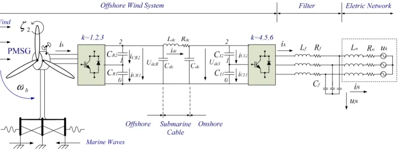
The OWS apart from the wind turbine has a rectifier linking a PMSG to a first set of two capacity banks. An HVDC transmission submarine cable links the first set of two capacity banks to a second one, which in turn is connected to an inverter in order to inject the energy into an electric network through a second order filter to reduce the higher harmonics content in the electric current. The topology of the OWS is shown in Fig. 2.

A. Marine Wave

The marine wave displacement acting on the floating platform can be modeled as in [13] as a convenient sum of harmonics and is given by

)] , , ( ) ( ) ( ) ( cos[ ) ( ) , , ( 1 t y x i i t i i t y x i a ϑ ζ ρ υ η η =

¦

+ − = . (1) where )) ( sin( )) ( cos( ) , , (x yt x _ψ i y _ψ i υ = + . (2)

where η is the wave displacement for x , y position as a function of time, the remaining variables are characteristics for the vector of harmonic waves, particularly, η_a is for amplitudes, _ϑ is for frequencies, _ζ is for phases (random), ρ

is for numbers, ψ is for directions.

The model used for describing the floating platform motion is the phase/amplitude model in which the marine wave displacement is considered to be the sum of enough number of harmonic waves.

b

ω

2

ζ

Figure 2. Offshore wind system with Three-level converter.

B. Turbine and Drive Train

The turbine mechanical power captured from the kinetic energy in the wind is given by

3

1 2

b p

P = φS u C . (3)

where P is the turbine mechanical power, S is the area b

covered by the turbine blades, φ is the air density, u is the average wind speed, Cp is the power coefficient.

The configuration of the simulated TM drive train is shown in Fig. 3.

e

ω

b

ω

Figure 3. TM drive train.

The equations for modeling the motion of the rotor for the TM drive train are based on the second law of Newton torsional version, given by

) ( 1 ah db ts msb b b b _{M M M M M} J dt d − − − + = ω _{. (4)} ) ( 1 e de ae mse ts e e _{M M M M M} J dt d − − − + = ω _{. (5)}

where ωb is the turbine rotor speed, J is the turbine moment b

of inertia, M is the mechanical torque, b Mmsb is the stiffness torque acting on the blades, hub and tower in the deep water,

ts

M is the torsional stiffness torque, Mdb is the turbine

bearing resistant torque, M is the airflow viscosity resistant ah

torque in the hub and blades, ωe is the PMSG rotor speed, J e

is the PMSG moment of inertia, M_mse is the stiffness torque on PMSG, M is the resistant torque in PMSG bearing, de M ae

is the airflow viscosity resistant torque in the PMSG, M is e

the electric torque. In Fig. 3 k_msb are k_mse are elastic coefficients due to the elastic behavior of the tower and the semisubmersible floating platform in deep water caused by the effect of the wave load [14,15].

C. PMSG

The equations for modeling a PMSG can be retrieved in diverse texts [16]. A condition for avoiding the demagnetization in the permanent magnet of the PMSG is imposed by setting a null value for the reference of the stator direct component electric current * ₀

sd

i = [9].

D. TLC

The TLC is a AC-DC-AC converter, equipped with twelve unidirectional commanded insulated gate bipolar transistors (IGBTs), considered as unidirectional and ideal, identified by

ik

S , used as a rectifier and with six similar IGBTs used as an

inverter. The groups of four IGBTs connected to the same phase constitute the leg k of the converter. A switching variable n with _k nk∈{0,1,2} is used to identify the IGBT i

state in the leg k of the three-level converter, determining the

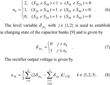
switching function of each IGBT. The switching variables [9] are given by ° ¯ ° ® ­ = = = = = = = 0 ) ( 1 ) ( , 0 0 ) ( 1 ) ( , 1 0 ) ( 1 ) ( , 2 4 3 2 1 4 1 3 2 2 1 4 3 k k k k k k k k k k k k k S e S e S e S S e S e S e S S e S e S e S n . (6)

The level variable δ_jnk with j∈{1,2} is used to establish the charging state of the capacitor banks [9] and is given by

¯ ® ­ ≤ > = k k jn _{j n} n j k ₁ 0 δ . (7)

The rectifier output voltage is given by

¦

¦

≠ = = − = 3 1 2 1 ) 2 ( 3 1 k l l CRj jn j jn sk U u l k δ δ k∈{1,2,3}. (8)

The state equation of the DC voltages at the first set of capacity bank, i.e., at the rectifier side, is given by

¦

=

+

=

2 1

1

j CRj dc Rj dcR

_i

C

C

dt

dU

. (9)

The linking between the first set of two capacity banks on offshore to a second one on onshore is assumed to be a HVDC transmission submarine cable. The impedance of the submarine cable is modeled by a π equivalent electric circuit model [16]. The current i in the submarine cable is given by _dc

) ( 1 dc dc dcI dcR dc dc _{U U R i} L dt di − − = . (10)

The DC voltage at the second set of capacity banks U_dcIj, i.e., at the inverter side, is given by

¦

= + = 2 1 1 j CIj dc Ij dcI _i C C dt dU . (11)

The inverter output voltage is given by

¦

¦

≠ = = − = 6 4 2 1 ) 2 ( 3 1 k l l CIj jn j jn sk U u l k δ δ k∈{4,5,6}_{. (12)} E. Electric Network

A three-phase balanced circuit models the electric network. The state equation for the current injected in the electric network is given by ) ( 1 k fk n fk n fk _{u R i u} L dt di − − = k∈{4,5,6}_{. (13)}

III. CONTROL METHOD

The controllers used in the OWS are PI in order to obtain the reference currents in dq axes. The TLC is a variable structure, because of the transistors on/off switching state. Therefore, the SM control is important for adjusting the TLC, by ensuring the choice of the appropriate space vectors. Moreover, PWM by SVM supplemented with SM is used to trigger the IGBTs. Power transistors are not able to switch at infinite frequency due to physical limitations. So, an error e _αβ

will exist between the reference value and the control value. In order to verify that the system follows the sliding surface

( , )

A e_αβ t is necessary that the error trajectory in the neighboring of the sliding surface, observe the conditions [10] given by

( , ) ( , ) / 0

A e_αβ t dA e_αβ t dt< (14)

A small error is acceptable in practice and a convenient achievement of this strategy is accomplished with hysteresis comparators [12]. If the current error, given by the comparators hysteresis output, σ_αβ, is quantified in five levels is possible to relate the space vectors with the current error. So σ_αβ are integers numbers taking the values in the set {−2,−1,0,1,2}.

The output voltage vectors in the αβ coordinates, as well as the voltage level of phase 1, 2 and 3, respectively, for the TLC are shown in Fig. 4. For the TLC there are 27 output voltage vectors, which include 8 redundant ones.

Figure 4. Output vectors for the TLC.

The control strategy carries out a reduction on the capacitors banks unbalancing voltage by considering three vector tables, which take into account the charging state of each capacitor bank selecting the most appropriate voltage vector according to the voltage level of each converter leg, taking advantage of the redundant output voltage vectors. Table I, Table II and Table III summarizes the vector selection for level 0, level 1 and level 2, respectively.

IV. CASE STUDY

The simulated OWS has a nominal power of 2 MW. The mathematical model for the OWS with the TLC is implemented in Matlab/Simulink. The wind speed considered

is a ramp, with a speed between 5 m/s to 25 m/s and a time horizon of 5 s. The continuous voltage at the submarine cable is 5 kV.

TABLE I. OUTPUT VECTORS SELECTION FOR LEVEL 0

\ β α δ δ -2 -1 0 1 2 -2 3 3 12 21 21 0 6 2 2 20 20 0 9 5 1 10 19 1 8 4 4 22 22 2 7 7 16 25 25

TABLE II. OUTPUT VECTORS SELECTION FOR LEVEL 1 \ β α δ δ -2 -1 0 1 2 -2 3 3 12 21 21 0 6 15 11 11 20 0 9 5 14 23 19 1 8 17 13 26 22 2 7 7 16 25 25

TABLE III. OUTPUT VECTORS SELECTION FOR LEVEL 2 \ β α δ δ -2 -1 0 1 2 -2 3 3 12 21 21 0 6 6 24 24 20 0 9 9 27 23 19 1 8 8 26 26 22 2 7 7 16 25 25

The marine wave displacement is shown in Fig. 5.

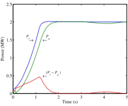
The results for the turbine mechanical power, the PMSG electric power and the accelerating power are shown in Fig. 6.

The results for the capacitors voltage at the rectifier side and the reference voltage are shown in Fig. 7.

The DC current at the submarine cable is shown in Fig. 8.

0 1 2 3 4 5 −15 −10 −5 0 5 10 15 Time (s) Surface elevation (m)

Figure 5. marine wave displacement

0 1 2 3 4 5 0 0.5 1 1.5 2 2.5 Time (s) Power (MW) → Pt ←Pg ←(Pt − Pg )

Figure 6. Mechanical power and electrical power.

0 1 2 3 4 5 0 1 2 3 4 5 6 7 Time (s) Voltage (kV) U_dc* U_CR1 U_CR2 U_dcR

Figure 7. Capacitor Voltage at the rectifier side and reference voltage.

0 1 2 3 4 5 −1 −0.5 0 0.5 1 1.5 2 Time (s) DC current (kA)

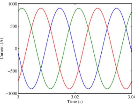
Figure 8. DC current at the submarine cable. The output current at the inverter is shown in Fig. 9.

3 3.02 3.04 −1000 −500 0 500 1000 Time (s) Current (A)

Figure 9. Output current at the inverter.

The current injected into the electric network after the action of the second order filter is shown in Fig. 9.

3 3.02 3.04 −1000 −500 0 500 1000 Time (s) Current (A)

Figure 10. Electric network injected current.

A comparison between Fig. 9 and Fig. 10 illustrates the suitable action taken by the second order filter.

In a previous study made by the authors [17,18], with a similar OWS equipped with a two-level converter the THD for a wind without perturbations is 2.43 %. The THD for the three-level converter is 0.5 %. A comparison of these values exposes the potentiality of the use of the multi-level converters in the improvement of harmonic content.

V. CONCLUSIONS

The increased penetration of wind energy implies research of mathematical models more realistic for offshore systems, particularly, in what regards wind energy offshore simulation. An integrated model for an offshore wind system with HVDC transmission is proposed, taking into consideration the dynamic associated with the action excited by the wind on all physical structure and assuming a wind turbine two mass drive train modeling. A case study is presented, simulating a three level converter topology for the integration of an offshore wind system linked to the electric network through a HVDC transmission submarine cable. The simulations carried out reveal that the model for the offshore wind system is adequate to reveal the performance of the system. Additionally, the case study proves that the offshore wind system can operate with an adequate performance.

ACKNOWLEDGMENT

This work is funded by Portuguese Funds through the Foundation for Science and Technology-FCT under the project LAETA 2015ϋ2020, reference UID/EMS/50022/2013.

REFERENCES

[1] SIEMENS:http://www.siemens.com/press/en/feature/2013/energy/2013-08-x-win.php?content%5B%5D=WP&content%5B%5D=

PS&content%5B%5D=EM&stop_mobi=true.

[2] F. Blaabjerg, and D.M. Ionel, “Renewable energy devices and systems – state-of the-art technology, research and development, challenges and future trends,” Electric Power Components and Systems, vol. 43 (12), pp. 1319-1328, July 2015.

[3] M P.S. Valverde, A.J.N.A. Sarmento, and M. Alves, “Offshore wind farm layout optimization—state of the art,” Journal of Ocean and Wind Energy, vol. 1, pp. 23-29, February 2014.

[4] A. Cordle, and J. Jonkman, “State of the art in floating wind turbine design tools,” in Proc. International Conference on Offshore and Polar Engineering, pp. 1-9, 2011.

[5] A. Ho, and A. Mbistrova, “The European offshore wind industry - key trends and statistics 1st half 2015," A report by the European Wind Energy Association - July 2015.

[6] A. Natarajan, "An overview of the state of the art technologies for multi-MW scale offshore wind turbines and beyond," WIREs Energy Environ, vol. 3, pp. 111-121, 2014.

[7] A. Arapogianni, and A-B. Genachte, "Deep water the next step for offshore wind energy," A report by the European Wind Energy Association, July 2013.

[8] M. Seixas, R. Melício, and V.M.F. Mendes, “Simulation of rectifier voltage malfunction on OWECS four-level converter, HVDC light link: smart grid context tool,” Energy Conversion and Management, vol. 97, pp. 140–153, June 2015.

[9] M. Seixas, R. Melício, and V.M.F. Mendes, “Fifth harmonic and sag impact on PMSG wind turbines with a balancing new strategy for capacitor voltages,” Energy Conversion and Management, vol. 79, pp. 721–730, March 2014.

[10] R. Melício, V.M.F. Mendes, and J.P.S. Catalão, “Modeling and simulation of wind energy systems with matrix and multilevel power converters,” IEEE Latin America Transactions, vol. 7(1), pp. 78-84, March 2009.

[11] M. Dicorato, G. Forte, and M. Trovato, “Wind farm stability analysis in the presence of variable-speed generators,” Energy, vol. 39, pp. 40-47, March 2012.

[12] E. Pican, E. Omerdic, D. Toal, and M. Leahy, “Direct interconnection of offshore electricity generators,” Energy, vol. 36, pp. 1543-1553, March 2011.

[13] F.N. Eikeland, "Compensation of wave-induced motion for marine crane operations,". Msc. Thesis, Norwegian University of Science; 2008, p. 16-26.

[14] J. Brooke, "Wave energy conversion systems," 1st Edition, Elsevier Science, UK, 2003.

[15] L.H. Holthuijsen, "Wave energy conversion systems," Cambridge University Press, Cambridge, UK, 2007, pp. 145 196.

[16] R. Melício, V.M.F. Mendes, and J.P.S. Catalão, “Wind turbines equipped with fractional-order controllers: stress on the mechanical drive train due to a converter control malfunction,” Wind Energy, vol. 14(1), pp. 13-25, January 2011.

[17] M. Seixas, R. Melício, V.M.F. Mendes, and H.M.I. Pousinho “Simulation of offshore wind system with two-level converters:HVDC transmission,” in Proc. International Power Electronics and Motion Control Conference and Exposition, pp. 1384-1389, 2014.

M. Seixas, R. Melício, V.M.F. Mendes, and C. Couto, “Blade pitch control malfunction simulation in a wind energy conversion system with MPC five-level converter,” Renewable Energy, vol. 89, pp. 339–350, April 2016.