Liquidity risk : an opportunity to open the window after closing a door

Carolina Perry da Câmara

April 2014

Abstract

Professor José Faias

Supervisor

Dissertation submitted in partial fulfillment of requirements for the degree of

Master of Science in Finance, at Universidade Católica Portuguesa, April 2014

Liquidity risk: An opportunity to

open the window after closing a door

Investors can incur in substantial losses if they cannot trade an asset at a desired price at a specific moment – this is liquidity risk. However, this may also pose as an advantage. We prove the relevance of liquidity in an investment strategy using liquidity both as a characteristic for investment decision and as an asset, through liquidity sorted portfolios. Liquidity provides significant improvements in investment performance, especially when allocating for small size stocks. After finding the significance of liquidity during recession periods but not during expansions, we propose a successful asset allocation strategy conditional on announcements timing of business cycles. Liquidity is relevant and you can profit from it – it is the open window when all the doors are closed.

Acknowledgments

First, I would like to thank my supervisor, Professor José Faias, for the constant support

and interest during these past months. Without his knowledge, guidance, patience and

comments it would not be possible to overcome all the dead-ends that we faced.

I would also like to extend my thanks to Católica Lisbon and all the Professors that

taught me not only Economics and Finance but also how to be professional and

hardworking, during my Undergraduate and Master’s Degree. I will never forget these

five wonderful years. I also wish to extend a special thanks to “Fundação para a Ciência

e Tecnologia”.

A sincere thanks to my Economic friends, João Pereira de Almeida and Ricardo Monteiro

for encouraging me to do my best. A special thanks to Pavel Onyshchenko, for providing

me such insightful advice on coding. To Marta Casqueiro, for being always there. And

to Marta Francisco, for her constant support and great friendship.

A special thanks to my Parents, for all their effort to provide me love and the best

education and my brothers and sister, for their true love. And to Martim, for always

believing in me and for his love.

Finally, a thanks to my grandparents, for all the days spent with them writing the thesis.

Especially to my Grandmother Lici, for her strength, and to my Grandfather Álvaro,

Contents

1

Introduction... 1

2

Market Illiquidity ... 4

3

Asset Allocation ... 7

4

Is Liquidity Relevant? ... 12

5

Is Liquidity Relevant In Times Of Information Uncertainty? ... 20

Index of Tables

Index of Figures

1

Introduction

From the beginning of the last recession period in the USA in December 2007, the Russell

3000 index, which represent 98% of the US stock market, exhibited a loss of 55% of its

value until September 2008. During this period, investors suffered severe losses and banks

faced liquidity constraints, as short term funding was more difficult and expensive. While

we are certain that liquidity issues existed in the corporate side, it is interesting to

understand whether liquidity played a role in the market turbulence throughout the

recession.1 _{More broadly, we aim to understand if investors can protect themselves and,}

even, benefit from controlling for liquidity in their investment decisions, not only in the

last financial crisis but in several past recession periods.

This dissertation finds empirical evidence that liquidity-based asset allocation provides

superior performance. More specifically, after defining an illiquidity measure, we prove the

relevance of liquidity information both as a decision element and as an asset, through the

use of liquidity sorted portfolios. For the purpose of the asset allocation, we prove that

liquidity is only relevant during recessions and based on this we propose a successful

investment strategy conditional on the NBER communications timing of economic cycles.

Pástor and Stambaugh (2003) define liquidity risk as the threat of not having the “ability

to trade large quantities quickly, at low cost, and without moving the price”. Amihud and

Mendelson (2012) present two types of liquidity costs: the first are direct trading cost and

the second - the one we focus our analysis on - is the price impact caused by a mismatch

between demand and supply for a given stock. However, liquidity risk is non observable.

Previous literature presents different measures to compute proxies for liquidity. Chordia et

al. (2001) use dollar trading volume and turnover. Amihud (2002) presents an illiquidity

measure, the average ratio of daily absolute return to the dollar trading volume. Pástor

and Stambaugh (2003) run regressions on liquidity-based information, such as volume, to

get a parameter that proxy for liquidity. Sadka (2006) propose a liquidity measure defined

as the price-impact induced by trades, using microstructure data. It is strongly accurate

but computationally intensive and has short availability of data. As shown by Goyenko et

al. (2009) low frequency measures (that do not use intraday data) have results close to high

frequency measures. We opt to compute Amihud (2002) illiquidity measure because of the

straightforward intuition and availability of data.

There is an extended literature on the importance of market liquidity in asset pricing.

Pástor and Stambaugh (2003) show that stocks with higher sensitivity to market liquidity

have higher expected returns, even when controlling for size, value and momentum factors.

Amihud (2002) and Datar et al. (1998) also prove the existence of an illiquidity premium,

especially for small size firms. Jones (2002) takes a step further by showing that liquidity

has predictive power over returns.

With the clear awareness of the impact of liquidity in the market performance, we

implement an investment strategy where we include two liquidity characteristics (both level

and change in liquidity) as well as other characteristics that have also shown predictive

power, such as the Term Spread or the Default Spread. We follow Brandt and Santa-Clara

(2006) in a dynamic model for asset allocation that linearly defines the weight of three

different assets (long-term bonds, short-term bonds and Stocks) using market

characteristics. We confirm the relevance of liquidity information as characteristics for two

US market index, both for large and small size firms. We decide to form five liquidity

portfolios and test the asset allocation with the extreme portfolios. We go further and we

(low liquidity portfolio) and Portfolio 5 (high liquidity portfolio) as investment assets in

the asset allocation strategies, providing gains by investing in the difference of liquidity.

But is liquidity relevant for all the periods? Chen et al. (2005) show that low liquidity

stocks only earn higher expected return when their default risk is also higher. It is intuitive

that the overall liquidity of the market is more relevant if there also exists pressure to sell

the assets, caused by a high default risk. Liu (2009) explains that investors only require

higher returns for illiquid stocks as the consumption risk increases during recessions. Also,

Beber et al. (2006) present that during stress periods, investors only care about liquidity

and not credit quality, leading to a “flight-to-liquidity” but not necessarily to quality,

creating devaluation in illiquid assets’ price despite the probability of default. Naes et al.

(2011) find empirical evidence of a strong relation between stock market liquidity and

business cycles, supporting that liquidity is a good predictor of economic crisis. Acharya et

al. (2013) show that the importance of liquidity is conditional on the state of the economy,

the same finding of Fujimoto and Watanabe (2005). To test these implications, we divide

the sample in two different periods, recession and expansions. We find no advantage in

including liquidity during expansions, both for small and large size stocks. During

recessions, however, there is a significant increase in performance. Using the conditional

relevance of liquidity, we propose an innovative conditional asset allocation. We use the

unconditional strategy for expansion periods and liquidity strategies for recession periods,

defined by NBER communications timing.

This dissertation introduces relevant insights to the importance of market liquidity risk by

(1) showing that market liquidity is a valuable characteristic that increases the performance

of an investment strategy, by exploiting the devaluation of illiquid assets, (2) including

liquidity as an asset dramatically increase the performance of asset allocation, using

economic cycles, using liquidity strategies only when they are significant – during

contraction periods.

The remainder of this dissertation is organized as follows. Section 2 presents the

methodology and data for the illiquidity measure while Section 3 presents the methodology

and data for the asset allocation. Section 4 presents the relevance of liquidity in asset

allocation, including liquidity as characteristic and asset. Section 5 proposes a conditional

strategy using NBER communications timing of business cycles and Section 6 concludes.

2

Market Illiquidity

Liquidity risk can be extremely costly for an investor, in the form of direct trading cost or

through the price impact, as evidenced by Amihud and Mendelson (2012). We focus our

analysis in the market price impact as it can lead to substantial unexpected losses.

Furthermore, as shown by Pástor and Stambaugh (2003) and Amihud (2002), market

liquidity has proven to significantly impact in asset pricing and to be a good predictor of

returns, as proved by Jones (2002). This reinforcing the relevance of studying liquidity.

2.1

Methodology

Liquidity risk reflects the inability to trade large quantities quickly, without moving the

price, at a lower cost. As it is not directly observable, Amihud (2002) develops an illiquidity

measure for the “daily price response associated with one dollar of trading volume”. If

liquidity is low, we expect a higher absolute return for a lower volume. Then the illiquidity

measure for each stock in calculated as follow:

𝐼𝑙𝑙𝑖𝑞𝑢𝑖𝑑𝑖𝑡𝑦𝑖,𝑚,𝑦 = 1 𝐷𝑖,𝑚,𝑦× ∑ |𝑟𝑖,𝑡,𝑚,𝑦| 𝑉𝑜𝑙𝑢𝑚𝑒𝑖,𝑡,𝑚,𝑦 𝐷𝑖,𝑚,𝑦 𝑡=1 (1)

where 𝐷_{𝑖,𝑚,𝑦} is the number of days of in month 𝑚, year 𝑦 with positive volume of company

𝑖 and 𝑟_{𝑖,𝑡,𝑚,𝑦} is the stock return on day 𝑡, on month 𝑚 of year 𝑦.

The market monthly illiquidity is given by:

𝐴𝐼𝑙𝑙𝑖𝑞𝑚,𝑦= 𝑀𝑚 𝑀1 × 1 𝑁𝑚,𝑦× ∑ 𝐼𝑙𝑙𝑖𝑞𝑢𝑖𝑑𝑖𝑡𝑦𝑖,𝑚,𝑦× 10 6 𝑁_𝑚,𝑦 𝑖=1 (2)

where 𝑁_𝑚,𝑦 is the number of companies for month 𝑚 of year 𝑦. We weigh the illiquidity

measure with the market value of the companies included in month 𝑚 on month 𝑚 − 1

(𝑀_𝑚), divided by the market value of companies on January 1962 (𝑀₁).2 _{We also compute}

the change in market illiquidity, by computing the difference of the natural logarithm:

∆𝐴𝐼𝑙𝑙𝑖𝑞𝑚,𝑦 = ln⁡(

𝐴𝐼𝑙𝑙𝑖𝑞𝑚,𝑦

𝐴𝐼𝑙𝑙𝑖𝑞𝑚−1,𝑦) (3)

2.2

Data

We compute the market illiquidity measure following Amihud (2002). We use CRSP Daily

File to retrieve daily individual stock return and volume. We adjust prices and shares for

stock splits and dividends distributions. Only common stocks are considered (share code 10

and 11). We use data from January 1962 to December 2012 and we exclude NASDAQ

companies.3 _{We only use stocks that exist in the last day of the previous year and had}

information on market capitalization.

We select companies with at least 200 observations in the previous year and with prices

above $5. We exclude observations in the 1% highest or lowest tails of the distribution in

the previous month.

2 _{The value of one dollar in 1962 is different from the value of one dollar today.}

The market illiquidity is highly persistent, showing a positive autocorrelation close to 0.8.

To better understand the influence of liquidity shocks we computed the change in illiquidity

that presents a negative autocorrelation of 0.25.

In Figure I, we take a closer look to the evolution of the illiquidity measure, and relate it

with recession periods, defined by NBER.

Figure I

Market Monthly Illiquidity evolution

This figure presents the monthly market illiquidity (Equation 2). All stocks used in the computation are from NYSE and AMEX. The number of companies changes every month, from 752 to 1,913 companies. We present the evolution from January 1962 to December 2012. The higher the market illiquidity, the higher the liquidity risk. The grey areas represent the recession periods, defined by NBER.

Naes et al. (2011) find empirical evidence of the connection between liquidity and business

cycles.The monthly evolution of market illiquidity is in line with their conclusion, with the

market presenting a higher level of illiquidity in crisis periods. More specifically, most of

the recession periods are combined with an increase of the market illiquidity. It is the case

of the first oil crisis (1973-1975) that present a significant illiquidity, as well as the second

oil shock (1990), the dot-com bubble (2001) or the last subprime crisis (2007-2009). This

is an important relation, between market illiquidity and recession periods. Several authors

as Acharya et al. (2013) or Fujimoto and Watanabe (2005) present the importance of

liquidity as being conditional on the economic environment, being considerably more

significant during recession periods. This is the case because of the increase in consumption

risk during downturns, as discussed by Liu (2009). The computation of the market

0 5 10 15

illiquidity reinforce the connection between recessions and illiquidity, both level and change.

This link is crucial for our study, since we aim to understand if we can improve the

performance of our strategy using the relevance of liquidity, particularly during recessions.

3

Asset Allocation

We aim to understand if liquidity information improves the performance of an investment

strategy. Jones (2002) finds empirical evidence of the predictive power of liquidity over

returns, as well as Amihud (2002).

3.1

Methodology

Following Brandt and Santa-Clara (2006), we allocate between a combination of different

asset types: stocks, long-term and short-term bonds. The allocation decision is a function

of a set of asset characteristics that maximize the expected utility of the investor. The main

advantage of the strategy is that the weights of each asset depend linearly on 𝐽 asset

characteristics 𝑥_𝑗,𝑡.

𝑤𝑖,𝑡= 𝜃0+ ∑ 𝜃𝑗,𝑡𝑥𝑗,𝑡 𝐽

𝑗=1

(4)

For each month 𝑡, we maximize the expected utility of the investor’s wealth.

⁡𝑈 =(1 + 𝑟𝑝) 1−𝛾

1 − 𝛾 , 𝛾 ≠ 1 (5)

where 𝑟_𝑝 is the portfolio return and 𝛾 the coefficient of risk aversion. We use a power utility

function, as it takes into account all moments of distribution and not only the mean and

standard deviation. Rosenberg and Engle (2002) and Tarashev and Tsatsaronis (2006) show

from option prices that the implicit risk aversion coefficient is between 2 to 8. We consider

estimated parameters and the consequent increase in precision. In addition, we do not need

to make any assumption on the distribution of the returns.

As for the characteristics, we use two different sets. The first (which we designate in short

by BSC onwards) uses the same characteristics used in Brandt and Santa-Clara (2006): the

Dividend-Price ratio (D/P), the Term Spread (TS), the Default Spread (DS) and the

relative T-Bill (RTB). The D/P is the log of the ratio of dividends over price, the TS is the

difference between the long term bond rate and the 3-Month Treasury Bill, the DS is the

difference between the BAA-rated bonds and AAA-rated bonds and the RTB is the

1-month Treasury Bill minus the last year average. All these variables have proven to have

good predictive power over returns. Fama and French (1989) empirically find that Dividend

Price ratio not only forecast returns for stocks but also for bonds as well as Term spread

and Default spread. The same results were confirmed by Chordia et al. (2001) and Keim

and Stambaugh (1986). Also, these variables have proven to be related to business cycles,

as evidenced by Fama and French (1988) or Keim and Stambaugh (1986).

The second set includes the level and the change in market illiquidity. We include liquidity

as a characteristic, as it also seems to be a good predictor of returns, as shown by Baker

and Stein (2004) or Jones (2002). Additionally, Naes et al. (2011) prove the predictive

power of liquidity over business cycles, reinforcing the importance of liquidity during

recessions. Finally, Goyenko and Ukhov (2009) prove that the illiquidity of stock market

has predictive power over bond market.

We rebalance our portfolio monthly, using an expanding estimation. We consider an initial

and compare the results mainly looking at the OOS results. However, we only consider a

strategy as consistently superior when beats its benchmarks both In and Out of Sample.4

3.2

Data

Our strategy allocates between three types of assets: short-term bonds, long-term bonds

and stocks. We use different proxies for the stocks. We use the Russell 2000 (small size

firms stocks) and Russell 3000 (all stocks) indexes, all retrieved from Bloomberg. Amihud

(2002) finds that the impact of market illiquidity is higher for small size firm. By using the

two indexes, we can better understand the relevance of liquidity-based strategies when

allocating for different size firms. All the returns are monthly, from February 1979 to

December 2012. We also form five liquidity portfolios, using the extreme portfolios as

proxies for stock index in asset allocation. Using the illiquidity information of past month,

each month we split the stocks used in the computation of illiquidity into five equally

weighted portfolios. Portfolio 1 contains the less liquid stocks and portfolio 5 contains the

most liquid stocks. This allow us to use liquidity as an asset. For short-term bonds, we use

the 1-month Treasury bill from Fama-French Factors. For the long-term bonds we retrieve

the long term rate from Goyal and Welch database.5 _{All the returns are monthly, from}

February 1962 to December 2012, and adjusted for stock splits and dividend distribution.

We define the weights for each asset using market characteristics. For BSC characteristics,

we retrieved the three characteristics Default Price ratio, Default Spread and Term Spread

from the Goyal and Welch database and the 1-month T-Bill from the Fama-French monthly

Factors. For the liquidity related characteristics, we consider both the level and change of

4 _{For space reasons, we comment on the In Sample performance but we decided not to present the results. However, the}

results are available and we can provide them upon request.

the computed illiquidity measure. All the characteristics are standardized for a better

comparison between the results of the different strategies using an expanding window.

We present the summary statistics for returns of each asset in Table I. To better understand

the influence of liquidity with respect to size, we choose to present the results of the Russell

2000 and Russell 3000 indexes and leave the S&P 500 index for robustness tests. The Russell

2000 and the Russell 3000 indexes are only available from 1984 onwards.

Table I

Summary Statistics for the Assets

This table presents the summary statistics for the assets used in the allocation, for two different estimation periods. We present the summary statistics from March 1967 to December 2012 for Portfolio 1 (low liquidity stocks), Portfolio 5 (high liquidity stocks), short-term bonds (1 Month Treasury Bill) and long-term bonds (Long Term rate). We also present the summary statistics for the Russell 2000 (small size stocks) and the Russell 3000 (all stocks) indexes, from March 1984 to December 2012. The results for short-term bonds and long-term bonds are similar for the second period, and so we opt not to present. Average, standard deviation and Sharpe ratios are annualized.

Summary Statistics

P1 P5 LT Bond ST Bond Russell 2000 Index Russell 3000 Index

Average (%) -3.60 1.98 8.31 5.18 7.06 7.48 St. deviation (%) 21.19 16.90 10.73 0.89 20.21 15.96 Sharpe ratio -0.41 -0.19 0.29 - 0.15 0.21 Skewness -0.71 -0.86 0.38 0.57 -1.22 -1.03 Excess Kurtosis 5.34 2.90 2.36 0.92 4.79 3.47 Minimum (%) -36.80 -26.95 -11.24 0.00 -36.77 11.84 Maximum (%) 28.41 14.20 15.23 1.35 15.20 -25.67

We also present two different time periods ending in 2012, but starting in either 1967 or

1984. Notice that the long-term bond presented the best risk return relation, with

approximately the double Sharpe ratio when comparing to the Russell 2000 index, for

example. However, as evidenced by Markowitz (1952), we can gain from diversification by

investing in several assets with different returns and volatility patterns. Moreover, as we

allow for short selling, the strategies gain not only from positive returns but also from falls

in prices. We expect that an allocation between several assets provides an improvement in

The standardize characteristics change every month of rebalancing. Therefore, we present

in Figure II the evolution of the characteristics, using the all sample for standardization.

Figure II

Evolution of standardize characteristics

This figure presents the evolution of the standardize characteristics (using all sample), from January 1962 to December 2012. In Panel A, we present the Dividend Price ratio, the log of ratio of dividends over price. Panel B presents the Default Spread, the difference between the BAA-rated bonds and AAA-rated bonds. Panel C presents the Term Spread, the difference between the long term bond rate and the 3-Month Treasury Bill. Panel D presents the relative T-Bill, the 1-Month Treasury Bill minus its 12-month average. Panel E presents the market illiquidity (Equation (2)) while Panel F presents the change in market illiquidity (Equation (3)). A: Dividend Price ratio B: Default Spread

C: Term Spread D: Relative T-Bill

E: Market Illiquidity F: Change in Market Illiquidity

We calculate the correlation between the six characteristics, and the BSC characteristics

present low correlation with liquidity characteristics but more significant between each

other. This suggest that liquidity information (both level and change) introduces new

information with respect to the other characteristics. Furthermore, the correlation

significantly increases if we only consider recession periods. Specifically between illiquidity

characteristics and Default Spread and Term Spread, sustaining the evidence to a

connection between liquidity and default. -10,0 -7,5 -5,0 -2,5 0,0 2,5 5,0 7,5 10,0 1962 1967 1972 1977 1982 1987 1992 1997 2002 2007 2012 -10,0 -7,5 -5,0 -2,5 0,0 2,5 5,0 7,5 10,0 1962 1967 1972 1977 1982 1987 1992 1997 2002 2007 2012 -10,0 -7,5 -5,0 -2,5 0,0 2,5 5,0 7,5 10,0 1962 1967 1972 1977 1982 1987 1992 1997 2002 2007 2012 -10,0 -7,5 -5,0 -2,5 0,0 2,5 5,0 7,5 10,0 1962 1967 1972 1977 1982 1987 1992 1997 2002 2007 2012 -10,0-7,5 -5,0 -2,5 0,0 2,5 5,0 7,5 10,0 1962 1967 1972 1977 1982 1987 1992 1997 2002 2007 2012 -10,0 -7,5 -5,0 -2,50,0 2,5 5,0 7,5 10,0 1962 1967 1972 1977 1982 1987 1992 1997 2002 2007 2012

4

Is Liquidity Relevant?

Our aim is to understand the value of liquidity information in asset allocation strategies.

We include liquidity information, using the market illiquidity and the change in it as

characteristics when allocating between different assets. First, we present results for two

different indexes, to better understand the impact in allocation when considering different

size stocks. We use the Russell 3000 index as a benchmark for the all market and the Russell

2000 index for small size stocks. Second, we use liquidity as an asset, by allocating on

liquidity sorted portfolios.

We perform seven different strategies. Strategy (0) is the unconditional strategy. Strategy

(1) uses the BSC characteristics (D/P ratio, Term Spread, Default Spread and Relative

T-Bill). Strategy (2) uses the level of market illiquidity while strategy (3) uses the change in

market illiquidity. Strategy (4) and (5) combines the BSC characteristics with the level of

market illiquidity or the change in market illiquidity, respectively. The last, strategy (6),

uses the level and change in market illiquidity simultaneously. We consider strategy (0)

and (1) as the benchmark strategies to compare with the performance of liquidity-based

strategies.

4.1

Using Liquidity As A Characteristic

A large number of authors reinforce the importance of liquidity in asset pricing and as a

predictor of future market returns (e.g. Pástor and Stambaugh (2003), Amihud (2002),

Datar et al. (1998), Jones (2002)). Based on these results, we test if the inclusion of liquidity

information provide better performance than an unconditional strategy, using the Russell

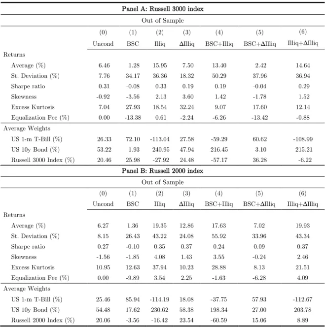
Table II

Comparison Performance Out of Sample

This table presents the results for each strategy OOS. We rebalance the portfolio monthly, using an initial expanding window of 5 years and a level of risk aversion of 4. The results are from February 1984 to December 2012. We allocate between the US 1-m T-Bill, the US 10y Bond and a stock index. Results for the Russell 3000 index are presented in Panel A while for the Russell 2000 index are presented in Panel B. The equalization fee is the yearly fee that the investor would pay to be able to use the conditional strategies over the conditional. Mean, standard deviation and Sharpe ratio are annualized.

We present the results for the Russell 3000 index in Table II Panel A. The IS results show

that all the strategies – except strategy (2) – that use liquidity outperform the ones that

do not account for it. Particularly, strategy (1) exhibit worse results then the unconditional

strategy. All the liquidity strategies present higher average return, but also with a

Panel A: Russell 3000 index Out of Sample

(0) (1) (2) (3) (4) (5) (6) Uncond BSC Illiq ∆Illiq BSC+Illiq BSC+∆Illiq Illiq+∆Illiq Returns Average (%) 6.46 1.28 15.95 7.50 13.40 2.42 14.64 St. Deviation (%) 7.76 34.17 36.36 18.32 50.29 37.96 36.94 Sharpe ratio 0.31 -0.08 0.33 0.19 0.19 -0.04 0.29 Skewness -0.92 -3.56 2.13 3.60 1.42 -1.78 1.52 Excess Kurtosis 7.04 27.93 18.54 32.24 9.07 17.60 12.14 Equalization Fee (%) 0.00 -13.38 0.61 -2.24 -6.26 -13.42 -0.88 Average Weights US 1-m T-Bill (%) 26.33 72.10 -113.04 27.58 -59.29 60.62 -108.99 US 10y Bond (%) 53.22 1.93 240.95 47.94 216.45 3.10 215.21 Russell 3000 Index (%) 20.46 25.98 -27.92 24.48 -57.17 36.28 -6.22

Panel B: Russell 2000 index Out of Sample

(0) (1) (2) (3) (4) (5) (6) Uncond BSC Illiq ∆Illiq BSC+Illiq BSC+∆Illiq Illiq+∆Illiq Returns Average (%) 6.27 1.36 19.35 12.86 17.63 7.02 19.93 St. Deviation (%) 8.15 26.43 43.22 24.08 55.92 33.96 43.34 Sharpe ratio 0.27 -0.10 0.35 0.37 0.24 0.09 0.37 Skewness -1.56 -1.85 4.08 1.43 3.55 -0.24 2.46 Excess Kurtosis 10.95 12.63 37.94 10.23 28.88 8.13 21.51 Equalization Fee (%) 0.00 -9.89 3.54 2.25 -1.63 -6.28 4.09 Average Weights US 1-m T-Bill (%) 25.46 85.94 -114.19 18.08 -37.75 57.93 -112.67 US 10y Bond (%) 54.48 17.62 230.62 58.38 198.34 27.00 203.78 Russell 2000 Index (%) 20.06 -3.56 -16.42 23.54 -60.59 15.06 8.89

significant increase in volatility. It is then crucial to evaluate the risk return relation, using

Sharpe ratio. Strategy (2) provides the best OOS Sharpe ratio, providing a little increase

when compared with the unconditional strategy (0), of approximately 6%.6 _{This is an}

expected result, since Amihud (2002) show that liquidity is more relevant for smaller stocks

and we are allocating mainly for larger stocks. Additionally, this strategy exhibits positive

skewness, being the probability of positive return higher than negative returns.

Furthermore, the cumulative return is three times superior when compared to the strategy

(0). However, notice from the equalization fee that the value for the investor of the

conditional strategy over the unconditional is almost insignificant and may disappear if the

transaction costs are higher than the equalization fee.

As a natural path, we perform the same asset allocation strategies but considering the

Russell 2000 index, a small cap index. When we look to Table II Panel B, the improvements

are considerably more significant. Again, liquidity strategies present a higher return also

with higher volatility. Strategy (3) and (6) improve the Sharpe ratio in comparison with

the unconditional and BSC strategy, both IS and OOS. The results of strategy (6) are

especially relevant, presenting an increase of 35% in the Sharpe ratio from the strategy (0)

as well as positive skewness. The cumulative performance is more than five times superior

to strategy (0).

The main difference on the strategies performance, for both indexes, relies on the allocated

weights. First, strategy (0) does not take advantage of short selling. Second, liquidity

strategies present a significant change of the weights during recessions. Particularly, the

success of the strategies come from the fact that the best strategies in both the Russell 2000

and the Russell 3000 indexes short sell short term bonds and buy long term bonds during

6_{Strategy (2) presents a slightly worse IS Sharpe ratio in comparison with the benchmark strategies. However, the benchmark}

recession periods. Amihud and Mendelson (2012) say that a rise in illiquidity generate a

flow from illiquid assets to more liquid instruments – the well-known “flight-to-liquidity”.

Simply put, investors tend to rebalance their portfolios toward liquid and less risky assets

during economic turbulence as presented by Beber et al. (2006). Acharya et al. (2013) find

that the change from more illiquid instruments to liquid instruments creates an additional

depreciation in prices of illiquid instruments. However, the liquidity strategies are doing

the opposite, moving to less liquid assets during recessions, providing liquidity to the

market. The strategies are buying the assets that investors are selling at a fire sale. After

the liquidity shock, the assets tend towards their true value, providing significant increases

in profitability. This is in line with Acharya and Pederson (2005) and Amihud, Mendelson

and Pederson (2005) that conclude that a persistent liquidity shock is linked with

contemporaneous negative returns but predict future positive returns.

This results confirm our main hypothesis of the relevance of liquidity information in asset

allocation, especially when allocating for smaller size firms. We provide significant

improvement in investment strategies performance by providing liquidity to the market

during recessions, investing in less liquid assets that are temporarily strongly undervalued.

The liquidity strategies beat the benchmark strategies and the market performance.7

4.2

Using Liquidity As An Asset

From previous results, we conclude that the inclusion of liquidity information increases the

performance of an asset allocation strategy. What if we include liquidity not only as a

characteristic but also as an asset? We start by splitting the stocks between equally

7_{In results not reported we run several robustness checks. The first is performing the same application but using S&P 500}

index for an extended period. The results are in line with the Russell 3000 index, showing the significance of liquidity, especially the level. Second, we change the coefficient of risk aversion to 10 to consider a more averse agent. Again, the results do not change, with similar performance. Third, the results are robust to the change to a mean variance utility function. The best strategies are same but with a significant increase in volatility.

weighted portfolios using past month stock illiquidity, from 1 (less liquid) to 5 (more liquid)

and allocate for each of the portfolio. We present an extended period because of longer

availability of data for these portfolios. The results provide a better insight of the

importance of liquidity for different liquidity portfolios.

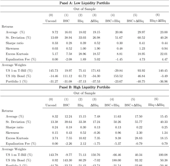
Table III

Comparison Performance Out of Sample

This table presents the results for each strategy OOS. We rebalance the portfolio monthly, using an initial expanding window of 5 years and a level of risk aversion of 4. We allocate between the US 1-m T-Bill, the US 10y Bond and liquidity equally-weighted portfolios. Panel A shows the results using Portfolio 1 (low liquidity portfolio) while Panel B shows the results using Portfolio 5 (high liquidity portfolio). The equalization fee is the yearly fee that the investor would pay to be able to use the conditional strategies over the conditional. Mean, standard deviation and Sharpe ratio are annualized.

Panel A: Low Liquidity Portfolio Out of Sample

(0) (1) (2) (3) (4) (5) (6) Uncond BSC Illiq ∆Illiq BSC+Illiq BSC+∆Illiq Illiq+∆Illiq Returns Average (%) 9.72 16.01 18.02 19.15 20.86 29.97 23.00 St. Deviation (%) 13.69 38.94 33.03 26.98 51.67 60.52 40.28 Sharpe ratio 0.33 0.28 0.39 0.52 0.30 0.41 0.44 Skewness 0.03 0.52 1.00 1.90 0.48 1.23 0.94 Excess Kurtosis 5.17 7.58 28.96 18.57 8.81 18.95 22.01 Equalization Fee (%) 0.00 -2.08 1.89 5.02 -1.45 4.73 4.47 Average Weights US 1-m T-Bill (%) 145.73 19.97 75.41 171.83 -29.84 93.92 140.45 US 10y Bond (%) -14.46 111.12 61.72 -34.30 153.52 46.84 -3.49 Portfolio 1 (%) -31.27 -31.08 -37.13 -37.53 -23.67 -40.75 -36.96

Panel B: High Liquidity Portfolio Out of Sample

(0) (1) (2) (3) (4) (5) (6) Uncond BSC Illiq ∆Illiq BSC+Illiq BSC+∆Illiq Illiq+∆Illiq Returns Average (%) 8.32 12.24 15.15 7.48 11.63 17.50 15.45 St. Deviation (%) 13.38 39.64 33.38 17.24 50.26 55.77 40.33 Sharpe ratio 0.24 0.18 0.30 0.13 0.13 0.22 0.25 Skewness 0.15 0.43 0.52 -0.26 0.96 2.30 1.24 Excess Kurtosis 3.74 7.55 10.82 7.35 9.38 28.83 18.15 Equalization Fee (%) 0.00 -2.26 2.12 -1.75 -5.37 -0.79 0.79 Average Weights US 1-m T-Bill (%) 143.78 -9.77 71.13 150.76 -66.46 40.34 100.08 US 10y Bond (%) 0.92 143.30 80.29 -7.02 188.00 92.32 50.38 Portfolio 5 (%) -44.70 -33.53 -51.42 -43.74 -21.54 -32.66 -50.46

Notice that in Table III Panel A, regarding Portfolio 1 (the most illiquid stocks), the main

results show that the liquidity change information increases the Sharpe ratio by

approximately 50%. Additionally, strategy (3) presents positive skewness and an

equalization fee of 5%. The average weights are close to the unconditional strategy. Almost

all the liquidity strategies beat OOS the unconditional strategy (except for strategy (2)),

reinforcing the importance of liquidity information. The results are in line with the existing

literature. According to Amihud and Mendelson (2012), market liquidity shocks are

especially relevant for low liquidity stocks, because the “flight-to-liquidity” phenomenon

intensifies the decline of low liquidity stock prices. Therefore, we can conclude that the

strategies with the best performance all include change in market illiquidity, being this the

most important factor when negotiating with low liquidity stocks.

From Portfolio 5 results presented in Table III Panel B, we prove that liquidity still plays

an important role but decreases it significance. The increase in the Sharpe ratio in strategy

(2) is much smaller (approximately 30%). Liquidity information is not as relevant as it was

in illiquid stocks, since liquidity risk for these stocks is not significant. Besides, the

“flight-to-liquidity” changes the allocation from less liquid securities to more liquid, meaning that

a negative effect caused by a shock in liquidity may be mitigated by the positive impact in

most liquid stocks, again shown by Amihud and Mendelson (2012) and so the final impact

is not clear. We conclude that for highly liquid stocks the market liquidity level is the best

characteristic to take into account in asset allocation strategies.

As expected, the results for Portfolio 1 are in line with the Russell 2000 index, and for

Portfolio 5 are in line with the Russell 3000. This suggest a strong relation between size

and liquidity proposing that small size stocks are less liquid, which is an expected result.

is higher information asymmetry, as mentioned by Amihud and Mendelson (2012),

increasing the mismatch between the price asked and the price offered.

We find evidence of difference between illiquid and liquid stocks. What if we invest in the

difference of liquidity? Our next step is to allocate between bonds and two different stocks:

the low and high liquidity stocks, through Portfolio 1 and 5. In fact, after proving the

influence of liquidity both in illiquid and liquid stocks, an asset allocation strategy assets

can gain from the difference by invests in both types of. We present the results for the asset

allocation in Table IV.

Table IV

Comparison Performance Out of Sample

In this table, we present the results for each strategy OOS, using an initial expanding window of 5 years and a level of risk aversion of 4. We present results from March 1967 to December 2012. We allocate between the US 1-m T-Bill, the US 10y, Portfolio 1 (low liquidity stocks) and Portfolio 5 (high liquidity stocks). The equalization fee is the yearly fee that the investor would pay to be able to use the conditional strategies over the conditional. Mean, standard deviation and Sharpe ratio are annualized.

First, we prove that all the strategies that use liquidity beat OOS the unconditional and

BSC strategies. As a result of the combination of illiquid and liquid stocks, we show that

both the level and change of market illiquidity are relevant. Nevertheless, only strategy (6)

simultaneously beats OOS and IS the benchmark strategies. This is an expected result and

Out of Sample

(0) (1) (2) (3) (4) (5) (6) Uncond BSC Illiq ∆Illiq BSC+Illiq BSC+∆Illiq Illiq+∆Illiq Returns Average (%) 10.12 39.72 32.20 32.84 68.98 99.82 53.56 St. Deviation (%) 15.79 94.95 60.63 44.23 151.20 180.85 84.47 Sharpe ratio 0.31 0.36 0.45 0.63 0.42 0.52 0.57 Skewness 0.07 4.61 1.70 0.40 5.15 5.96 2.30 Excess Kurtosis 7.45 48.79 22.52 18.05 57.49 59.93 22.01 Equalization Fee (%) 0.00 4.84 8.05 13.83 16.49 38.06 21.95 Average Weights US 1-m T-Bill (%) 146.59 8.65 86.46 205.96 -12.86 161.41 201.19 US 10y Bond (%) -1.84 122.01 47.59 -50.65 94.94 -4.80 -65.75 Portfolio 1 (%) -5.13 41.99 3.90 -36.98 100.64 53.05 -22.59 Portfolio 5 (%) -39.62 -72.66 -37.95 -18.33 -82.72 -109.66 -12.85

reinforces the relevance of the level of market illiquidity for liquid stocks and change in

market illiquidity for illiquid stocks. However, the greater improvement OOS in the Sharpe

ratio results from the inclusion of the change in market illiquidity information. Strategy (3)

presents an increase of approximately 75% and positive skewness. Moreover, the investor

would pay an annual fee of 13% to invest in strategy (3) instead of the unconditional

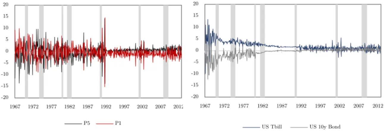
strategy. We present the evolution of the weights for this strategy in Figure III.

Figure III

Evolution of the weights, using Strategy (3)

This figure presents the weight evolution for strategy (3). Panel A present the evolution of weights for Portfolio 1 (low liquidity portfolio) and Portfolio 5 (high liquidity portfolio) while Panel B present for long-term bonds and short-long-term bonds. We present the evolution from March 2007 to December 2012. The grey areas are the recession periods, defined by NBER.

A: Portfolio 1 and Portfolio 5 B: Long-term bonds and short-term bonds

Notice in Figure III Panel A that the weights for each portfolio are almost perfectly

symmetric, with a correlation of approximately -0.97. From Panel B, the same happens but

with bonds, with a negative correlation of -0.94. This reinforce that the strategy is actually

investing on the difference of liquidity, both in equity market and bond market. With this

strategy’s weights, we are on average betting on a decrease of the stock market price,

especially for low liquidity stock that suffer a higher impact with liquidity shocks. We also

strongly invest in short-term bonds. This is a sign of the “flight-to-liquidity” phenomenon,

-20 -15 -10 -5 0 5 10 15 20 1967 1972 1977 1982 1987 1992 1997 2002 2007 2012 P5 P1 -20 -15 -10 -5 0 5 10 15 20 1967 1972 1977 1982 1987 1992 1997 2002 2007 2012 US Tbill US 10y Bond

as on average the strategy allocates more weight for the liquid assets and short sells the

assets that are expected to decrease the price thanks to the increase in liquidity risk.

We provide further evidence on the relevance of market liquidity. By introducing liquidity

not only as a characteristic but also as an asset, we strongly increase the performance of

our strategy in 75%, by investing in the difference of liquidity in the equity and bond

market.

5

Is Liquidity Relevant In Times Of Information Uncertainty?

There is evidence of a significant impact of liquidity in crisis periods. Acharya et al. (2013)

show that the impact of liquidity shocks is conditional on the economical conditions. The

same concludes Liu (2009), by showing that contractions in liquidity are clearly associated

with economic events and that liquidity risk is only relevant during consumption restraints.

We expect the relevance of liquidity to be clearer during recessions. However, the effect on

expansion periods is not clear.

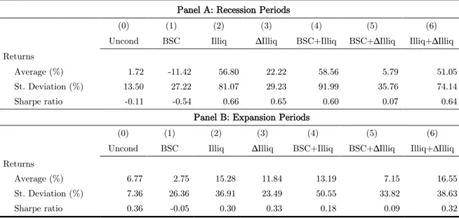
It is then crucial to understand the performance of the strategies during recession periods.

For that purpose, we first divide the performance of each strategy between recession and

expansion periods, for both the Russell 3000 index and the Russell 2000 index. Second, we

perform a conditional strategy on the economic situation. After a close analyses of the

relevance of liquidity depending on the business cycles, we test an innovative conditional

strategy using NBER communications timing. Essentially, after concluding that liquidity

is only relevant during recessions, we use a two regime strategy. When NBER announces

the end of recession, we use the unconditional strategy. When NBER announces the

beginning of a recession, we change to one of the liquidity strategies and only return to the

unconditional strategy when NBER announces the end of the recession. This way, we only

5.1

Recessions And Expansions: Is Liquidity Always Relevant?

We aim to test whether the relevance of liquidity is conditional on the business cycle. In

Table V we present the asset allocation strategies results, divided in expansion and

recessions for the Russell 3000 index.

Table V

Performance OOS of each strategy for the Russell 3000 Index,

divided by recession and expansions

This table presents the performance of each strategy OOS. We rebalance the portfolio monthly, using an initial expanding window of 5 years and a level of risk aversion of 4. The results are from February 1984 to December 2012. We allocate between the US 1-m T-Bill, the US 10y Bond and the Russell 3000 index. The results are divided by contraction periods (Panel A) and expansion periods (Panel B). These periods are defined using NBER information for the US business cycle. We consider 34 months of recession and 313 of expansion. The equalization fee is the yearly fee that the investor would pay to be able to use the conditional strategies over the conditional. Mean and standard deviation are annualized.

During recession, the strategies that include liquidity are always better than the

unconditional and the BSC strategies, except for strategy (3). It is important to highlight

the considerably better performance of strategies that include the level of liquidity. The

Sharpe ratio of the Russell 3000 index was -1.05, meaning that we also beat the market by

a large margin. However, during expansions, none of the liquidity strategies outperform the

unconditional strategy, showing signs of its irrelevance during times where liquidity is not

needed. The better strategies during crisis are the ones that use level of liquidity. This is

Panel A: Recession Periods

(0) (1) (2) (3) (4) (5) (6) Uncond BSC Illiq ∆Illiq BSC+Illiq BSC+∆Illiq Illiq+∆Illiq Returns

Average (%) 0.21 -0.06 37.70 1.36 58.95 3.72 31.47 St Deviation (%) 13.15 35.24 66.69 17.78 93.84 40.53 65.55 Sharpe ratio -0.23 -0.09 0.52 -0.11 0.59 0.01 0.43

Panel B: Expansion Periods

(0) (1) (2) (3) (4) (5) (6) Uncond BSC Illiq ∆Illiq BSC+Illiq BSC+∆Illiq Illiq+∆Illiq Returns

Average (%) 7.14 1.43 13.58 8.17 8.46 2.27 12.81 St Deviation (%) 6.93 34.11 31.48 18.40 43.03 37.74 32.49 Sharpe ratio 0.43 -0.08 0.30 0.22 0.10 -0.05 0.27

reinforce our previous findings, showing that for large size stocks the explanatory power of

liquidity comes from its level and not change. To better test the hypothesis of the

irrelevance of liquidity during expansion periods, we perform the same exercise for the

Russell 2000 index.

Table VI

Performance OOS of each strategy for the Russell 2000 Index,

divided by recession and expansions

This table presents the performance of each strategy OOS. We rebalance the portfolio monthly, using an initial expanding window of 5 years and a level of risk aversion of 4. The results are from February 1984 to December 2012. We allocate between the US 1-m T-Bill, the US 10y Bond and the Russell 2000 index. The results are divided by contraction periods (Panel A) and expansion periods (Panel B). These periods are defined using NBER information for the US business cycle. We consider 34 months of recession and 313 of expansion. The equalization fee is the yearly fee that the investor would pay to be able to use the conditional strategies over the conditional. Mean and standard deviation are annualized.

In Table VI Panel A, we present the results for recessions using the Russell 2000 index. All

the liquidity strategies outperform the benchmark strategies. The Sharpe ratio of the

market was -0.80 which is much lower than the one presented by liquidity strategies during

the recession periods, with strategy (2), (3) and (6) showing very close performances. For

expansions, we have the same result as before, as the unconditional is the best strategy.

However, strategy (2) and (6) present a close performance to strategy (0), suggesting that

during expansions, market illiquidity is more relevant for small firms than for large firms.

Panel A: Recession Periods

(0) (1) (2) (3) (4) (5) (6) Uncond BSC Illiq ∆Illiq BSC+Illiq BSC+∆Illiq Illiq+∆Illiq Returns

Average (%) 1.72 -11.42 56.80 22.22 58.56 5.79 51.05 St. Deviation (%) 13.50 27.22 81.07 29.23 91.99 35.76 74.14 Sharpe ratio -0.11 -0.54 0.66 0.65 0.60 0.07 0.64

Panel B: Expansion Periods

(0) (1) (2) (3) (4) (5) (6) Uncond BSC Illiq ∆Illiq BSC+Illiq BSC+∆Illiq Illiq+∆Illiq Returns

Average (%) 6.77 2.75 15.28 11.84 13.19 7.15 16.55 St. Deviation (%) 7.36 26.36 36.91 23.49 50.55 33.82 38.63 Sharpe ratio 0.36 -0.05 0.30 0.33 0.18 0.09 0.32

These results confirm two of our hypotheses. First, that liquidity plays a special role during

crises. In particularly, Acharya et al. (2013) show that the impact of liquidity shocks in

assets is conditional, being considerably higher during recessions and that there is a

“flight-to-liquidity” that strengthen the decrease effect in small size stocks price while diminishes

the decrease – or even increase – the effect in large stock price. Beber et al. (2006) suggest

that credit quality matters for pricing during expansion periods but not during crises, where

the main role belongs to liquidity. Second, we find evidence that during expansions, the

better strategy is the unconditional, suggesting the irrelevance of liquidity when there are

no consumption restraints or default pressures.

5.2

Conditional Strategy Using NBER Communication Timing

From previous results, we conclude the relevance of liquidity under recession periods but

the insignificance of this information during expansion periods. Using the conclusion of

Acharya et al. (2013), on the conditional impact of liquidity on economic environment, we

decide to perform an investment strategy where we allocate unconditionally during

expansion periods (using strategy (0)) and change to liquidity strategies in recession periods.

However, it is not easy to clearly define the expansion or recession periods. To do so, we

use the periods defined as recession by NBER.8 _{In most of the cases, the communication of}

this information is lagged, sometimes by up to as much as a whole year. For example,

NBER define the last subprime crisis from December 2007 until June 2009. Though, the

announcement on the beginning of the recession was only on the December 1st_{, 2008 and of}

8_{“The NBER does not define a recession in terms of two consecutive quarters of decline in real GDP. Rather, a recession is}

a significant decline in economic activity spread across the economy, lasting more than a few months, normally visible in real GDP, real income, employment, industrial production, and wholesale-retail sales.”, NBER's Business Cycle Dating Committee.

the end on the December 20th_{, 2009. We use the communication timing and not the true}

periods of recession, to have all the information out of sample.

With the definition of recession periods using NBER communications timing, we perform

our investment strategy. When NBER announces that US economy is under a recession,

we change the strategy in the end of the month of communication to a liquidity strategy.

When NBER announces the end of the recession, and the consequent beginning of an

expansion, we return to the unconditional strategy at the end of the month of

announcement. The investment strategy is then conditional on the US economy

environment. Essentially, we are using a strategy that takes into account liquidity when it

is more relevant, during contractions, as argued by Liu (2009). During expansions, we have

already shown that liquidity information does not increase the performance of the portfolio,

so we change to the unconditional strategy in those periods.

We perform the conditional strategy both for the Russell 2000 index and the Russell 3000

index that clearly show a fit in the allocation during recession periods. Strategies (0) to (6)

are the same as before. Strategy (0)+(2) is the use of the unconditional strategy in

expansions and the level of market illiquidity in recessions while (0)+(3) uses the change

of market illiquidity in recessions. Strategy (0)+(4) uses the unconditional strategy in

expansions and the level of market illiquidity plus BSC during recessions, while (0)+(5)

uses changes in market illiquidity plus BSC during recessions. To finish, strategy (0)+(6)

uses the unconditional strategy during expansions and level and change in market illiquidity

during recessions.

We present results for the Russell 2000 index in Table VII. Notice that we have a small

increase in the Sharpe ratio with strategies (0)+(3) and (0)+(5), both of which use the

is more important than the level for small size firms. However, the increase is not significant

when compared to strategy (0) or (3). The main advantage is the decrease in the volatility

of the returns, but the increase in Sharpe ratio is not significant. This is expected as the

difference between liquidity strategies and the unconditional was not significant during

expansions for small size firms.

Table VII

Performance of each strategy, using NBER communications timing

This table presents the performance of each strategy OOS. We rebalance the portfolio monthly, using an initial expanding window of 5 years and a level of risk aversion of 4. We allocate between the US 1-m T-Bill, the US 10y Bond and the Russell 2000 index. The results are divided by the previous defined strategies (Panel A) and the communication strategies (Panel B). The recession periods are defined using NBER communication timing information for the US business cycle. We consider 61 months of recession and 286 months of expansion. The equalization fee is the yearly fee that the investor would pay to be able to use the conditional strategies over the conditional. Mean and standard deviation are annualized.

Nonetheless, when the same strategies are applied to the Russell 3000 index (Table VIII),

all the communication strategies show an increase in the Sharpe ratio in comparison with

strategy (0) and strategy (2). This result highlights the good performance of an adaptive

strategy. Basically, we show that for the whole market - both small and large size companies

- if we take into consideration the market illiquidity between communications of beginning

and ending of recessions from NBER, we can increase the Sharpe ratio performance. This

increase is due to a substantial decrease in the standard deviation of returns. As proven

Panel A: Asset Allocation Strategies (0) Uncond (1) BSC (2) Illiq (3) ∆Illiq (4) BSC+Illiq (5) BSC+∆Illiq (6) Illiq+∆Illiq Returns Average (%) 6.27 1.36 19.35 12.86 17.63 7.02 19.93 St Deviation (%) 8.15 26.43 43.22 24.08 55.92 33.96 43.34 Sharpe ratio 0.27 -0.10 0.35 0.37 0.24 0.09 0.37

Panel B: Conditional Investment Strategy

(0)+(2) (0)+(3) (0)+(4) (0)+(5) (0)+(6) Returns

Average (%) 8.32 9.90 9.86 11.39 7.44 St Deviation (%) 13.35 15.23 16.89 19.51 11.70 Sharpe ratio 0.32 0.38 0.34 0.38 0.29

before, the liquidity strategies in general provide higher returns but with higher risk. When

we adopt the conditional asset allocation we decrease the volatility of the strategy, as we

use the unconditional strategy most of the time.

Table VIII

Performance of each strategy, using NBER communications timing

This table presents the performance of each strategy OOS. We rebalance the portfolio monthly, using an initial expanding window of 5 years and a level of risk aversion of 4. We allocate between the US 1-m T-Bill, the US 10y Bond and the Russell 3000 index. The results are divided by the previous defined strategies (Panel A) and the communication strategies (Panel B). The recession periods are defined using NBER communication timing information for the US business cycle. We consider 61 months of recession and 286 months of expansion. The equalization fee is the yearly fee that the investor would pay to be able to use the conditional strategies over the conditional. Mean and standard deviation are annualized.

This result reinforces the conclusions of Chen et al. (2005) concerning the relevance of

liquidity when the markets are under stress because of higher probability of default. With

higher probability of default, we have a consumption pressure and so there is a flight from

illiquid to liquid stocks creating pressure to sell illiquid stocks and buy liquid assets, also

pressuring the prices.

We propose an adaptive strategy which only consider liquidity when it is mostly needed.

The results confirm that the application of an investment strategy that only uses liquidity

information during recessions provides an increase the strategy performance, by reduction

of the volatility.

Panel A: Asset Allocation Strategies (0) Uncond (1) BSC (2) Illiq (3) ∆Illiq (4) BSC+Illiq (5) BSC+∆Illiq (6) Illiq+∆Illiq Returns Average (%) 6.46 1.28 15.95 7.50 13.40 2.42 14.64 St Deviation (%) 7.76 34.17 36.36 18.32 50.29 37.96 36.94 Sharpe ratio 0.31 -0.08 0.33 0.19 0.19 -0.04 0.29

Panel B: Communication Investment Strategies

(0)+(2) (0)+(3) (0)+(4) (0)+(5) (0)+(6) Returns

Average (%) 8.89 9.60 11.06 12.40 10.89 St Deviation (%) 13.38 14.48 18.86 20.49 18.51 Sharpe ratio 0.36 0.38 0.37 0.41 0.37

6

Conclusion

The 2007 recession motivated us to study the topic of market liquidity, taking into

consideration the substantial losses in the US equity market. Our main challenge was to

measure it and, by incorporating it in investment decisions, reduce losses or even provide

profits for the investors.

This dissertation introduces insightful contributions on the relevance of market liquidity

under asset allocation strategies. We find that the inclusion of liquidity risk information as

a characteristic in asset allocation increases the performance of the strategies, especially for

small size firms. Moreover, we decide to consider liquidity not only as informative but also

as an asset. To do so, we split stocks into five liquidity sorted portfolios and consider each

individually as investment assets, proving that liquidity characteristics provide better

performance when allocating for the low liquidity portfolio. We take a step further and

consider the least and most liquid portfolios as investment assets simultaneously, proving

that the difference in assets’ liquidity provides a 75% increase in Sharpe ratio.

To fully accomplish the aim of our study, we divide our sample between recession and

expansion periods and we empirically find that liquidity is only relevant during recession

periods. Thus, we improve the performance of the asset allocation by proposing an

innovative and successful strategy conditional on the business cycle announcements timing

of NBER. More specifically, this strategy is a combination of the unconditional strategy

during expansions with liquidity strategies in recession periods.

Our results show a clear relevance of market liquidity in providing better investment

strategy performance, fundamentally during recession periods. Liquidity is the open window

References

Acharya, V., & Pedersen, L., 2005. Asset pricing with liquidity risk. Journal of Financial Economics 76, 375-410.

Acharya, V., Amihud, Y., & Bharath, S., 2013. Liquidity risk of corporate bond returns: A conditional approach. Journal of Financial Economics 110, 358-386.

Amiduh, Y., 2002. Illiquidity and stock returns: Cross-section and time-series effects. Journal of Financial Markets 5, 31-56.

Amihud, Y., & Mendelson, H., 2012. Liquidity, the value of the firm, and corporate finance.

Journal of Applied Corporate Finance 24, 17-32.

Amihud, Y., Mendelson, H., & Pedersen, L., 2005. liquidity and asset prices. Foundations and trends in Finance 1, 269-364.

Baker, M. & Stein, J., 2004. Market liquidity as a sentiment indicator. Journal of Financial Markets 7, 217-299.

Beber, A., Brandt, M., & Kavajecz, K., 2006. Flight-to-liquidity or flight-to-quality? Evidence from the euro-area bond market. Review of Financial Studies 22, 925-957

Chen, J., Vassalou, M., & Zhou, L., 2005. The interrelation of liquidity risk, default risk, and equity returns. Working Paper.

Chordia, T., Roll, R., & Subrahmanyam, A., 2001. Market liquidity and trading activity.

Journal of Finance 56, 501-530.

Chordia, T., Subrahmanyam, A., & Anshuman, V., 2001. Trading activity and expected stock returns. Journal of Financial Economics 59, 3-32.

Datar, V., Naik, N., & Radcliffe, R., 1998. Liquidity and stock returns: An alternative test.

Journal of Financial Markets 1, 203-219.

Fama, E. & French, K., 1988. Dividend yields and expected stock returns. Journal of Financial Economics 22, 3-25.

Fama, E. & French, K., 1989. Business conditions and expected returns on stocks and bonds.

Journal of Financial Economics 25, 23-49.

Fujimoto, A., & Watanabe, M., 2005. Liquidity and conditional heteroscedasticity in stock returns, Working Paper.

Goyenko, R., Holden, C., & Trzcinka, C., 2009. Do liquidity measures measure liquidity?

Journal of Financial Economics 92, 152-181.

Goyenko, R., Ukhov, A., 2009. Stock and bond market liquidity: A long-run empirical analysis.

Jones, C., 2002. A century of stock market liquidity and trading. Working Paper.

Keim, D. & Stambaugh, R., 1986. Predicting returns in the stock and bond markets. Journal of Financial Economics 17, 357-390.

Liu, W, 2009. Liquidity and asset pricing: Evidence from daily data over 1962 to 2005. Working Paper.

Markowitz, H., 1952. Portfolio Selection. The Journal of Finance 7, 77-91

Næs, R., Skjeltorp, J., & Ødegaard, B. A., 2011. Stock market liquidity and the business cycle.

The Journal of Finance 66, 139-176.

Pástor, L., & Stambaugh, R., 2003. Liquidity risk and expected stock returns. Journal of Political Economy 11, 642-685.

Rosenberg, J., & Engle, R., 2002. Empirical pricing kernels. Journal of Financial Economics 64, 341-372.

Sadka, K., 2006. Momentum and post-earnings-announcement drift anomalies: The role of liquidity risk. Journal of Financial Economics 80, 309-349.

Tarashev, N., & Tsatsaronis, K., 2006. Risk premia across markets: Information from option prices. BIS Quarterly Review 3, 93-103.