Optimal taxation policy in the presence of idiosyncratic risk

(1)

Optimal taxation policy in the presence of

idiosyncratic risk

Maria Madalena Alves Morais Borges

Dissertation written under the supervision of Professor Catarina Reis

Dissertation submitted in partial ful…llment of the requirements of the Master of Science in Economics

at the

Universidade Católica Portuguesa

(2)

(3)

Acknowledgments

First and foremost, I would like to thank my supervisor, Professor Catarina Reis, who made this work possible by providing unmeasurable help and aspiring guidance throughout the whole process.

Furthermore, I would like to express my sincere gratitude to Professor Pedro Teles and Professor Isabel Horta Correia, who helped me discover my passion for Macroeconomics.

I would also like to thank my family, friends and colleagues for the unfailing support and continuous encouragement over the last months.

Finally, I would like to thank God for making me a curious being and for granting me the capability to write this thesis.

(4)

(5)

Optimal taxation policy in the presence of idiosyncratic risk

Madalena Borges

Thesis supervisor: Professor Catarina Reis June 1, 2017

Abstract

This paper builds on the analysis of Panousi and Reis of a linear capital taxation model where households face undiversi…able capital income risk and labor income risk. It highlights the relevance of consumption taxes in this framework. This paper provides a theoretical and a numerical analysis of the optimal …scal policy in response to capital income shocks and labor income shocks. The results show that consumption taxes have the same capa-bility of providing insurance as capital income taxes, without the downside of a¤ecting the households’capital decision. In this setting, the consumption tax should be used to reduce the volatility in income and in consumption, and the optimal capital income tax is zero.

(6)

(7)

Optimal taxation policy in the presence of idiosyncratic risk

Madalena Borges

Thesis supervisor: Professor Catarina Reis June 1, 2017

Resumo

Esta tese alicerça-se no modelo de Panousi e Reis, no qual é determinada a forma óptima de tributar o capital num contexto em que existe incerteza relativamente ao retorno do capital e ao retorno do trabalho. É realçada a importância que a utilização de um imposto sobre o consumo pode ter neste âmbito. Esta tese deriva em termos teóricos e analisa numericamente a tributação óptima em resposta a choques no retorno do capital e no retorno do trabalho. Os resultados demonstram que a tributação do consumo constitui uma alternativa à tributação do capital, na medida em que permite reduzir a incerteza sem afectar a decisão óptima de capital. Neste modelo, a política …scal óptima consiste na utilização da tributação do consumo com o propósito de diminuir a volatilidade do rendimento das famílias e do seu consumo, juntamente com a não tributação do capital.

(8)

(9)

1 Introduction

Over the years, several economists have focused their work on optimal taxation problems. One recurrent result found in the literature is that capital income should not be taxed. For instance, Chamley (1986) has shown that, in general equilibrium models with in…nitely lived agents, the optimal capital income tax should be zero in the long run. On this matter, Lucas (1990) also argued that capital income should not be taxed. After looking at the data for the U.S., Lucas estimated that the elimination of the tax on capital income would increase signi…cantly the capital stock. Consequently, there would be welfare gains, even though these gains would be downsized due to diminishing returns on capital.

However, this result is not universally veri…ed. Several economists have shown that there are scenarios and market structures that justify the optimality of a capital income tax or capital income subsidy even in the long run. For instance, Aiyagari (1995) showed that the existence of incomplete insurance markets and borrowing constraints lead to a positive steady-state capital income tax. The sign of this tax is justi…ed by the fact that both these speci…cities induce savings and capital accumulation. Aiyagari proved it was optimal to set a positive capital income tax to reduce capital accumulation. Correia (1996) presented another exception to the “Chamley theorem” (1986). Correia showed that when there are no restrictions on the taxation of all factors of production, the zero tax on capital income remains optimal. However, whenever one of the production factors cannot be taxed directly, capital income tax should be di¤erent from zero. Finally, Panousi and Reis (2016) provided another framework where it is optimal to have capital income taxes di¤erent from zero in the long run. They showed that in the presence of idiosyncratic income risk capital income taxes can be used as insurance with the purpose of decreasing uncertainty in this model.

In this paper, we build on the Panousi and Reis (2016) stochastic model for a closed economy as we strive to understand if there is any alternative or complementary con…gura-tion of …scal policy that increases welfare in this economy. We will preserve the underlying assumption that the households’investment decision does not depend on the realization of uncertainty to keep the tractability of the model. On the contrary, the households’decision over consumption is made after the households have full information regarding the shocks they are subject to in the current period.

The theoretical and quantitative results of our work suggest a relevant role for the consumption tax in this model. We conclude that in the presence of uncertainty regarding capital income, the optimal …scal policy consists in the taxation of consumption as a mean to decrease volatility in consumption. Furthermore, contrary to what is veri…ed in Panousi

(12)

and Reis (2016), if the instability in income and in consumption is only induced by shocks in labor income there is a role for …scal policy. We can use consumption taxes constant over time to diminish the variability of consumption without distorting the investment decision. The paper proceeds as follows. In section 2, we describe our model, in particular we characterize the households, the …rms, the government and the markets. In section 3, we derive the competitive equilibrium solution for our stochastic model. Section 4 derives the …rst best for this economy. Section 5 solves the benevolent government’s problem to determine the optimal way to use …scal policy in order to maximize the welfare in our economy. In section 6, we subject our economy to capital income shocks and labor income shocks, individually and jointly, to analyze the optimal …scal policy in each framework. Finally, section 7 concludes.

2 The model

In this section, we consider a neoclassical stochastic model for a closed economy, which is a modi…ed version of Panousi and Reis (2016). Time is discrete and indexed by t. There is a continuum of identical in…nitely lived households of size unity. In each period, there is uncertainty regarding the remuneration of capital and the remuneration of labor. When a household is subject to an idiosyncratic capital income shock ( _t), its pre tax rate of return of capital may increase or decrease by an amount _t. Additionally, if a household faces a labor income shock ("t), it increases or decreases the household’s remuneration of

labor by "t. We maintain the simplifying assumption that the decision of capital investment

is made before the realization of uncertainty. Therefore, the income risk has an e¤ect on the consumption of households but not on the investment decision. Moreover, we consider that the income shocks ( _t and "t) are independent and identically distributed over time,

so that the expectations of the households are not in‡uenced by previous shocks. In this framework, we consider that the …rms are owned by households. However, we do not need to take into account pro…ts since we assume that …rms behave competitively and there are constant returns to scale in production. Lastly, we introduce an additional …scal instrument to the model of Panousi and Reis (2016): a non state contingent consumption tax. The purpose of this consumption tax is to increase e¢ ciency in our economy.

(13)

2.1 The households

Taking into consideration the assumption that households are identical prior to the real-ization of the uncertainty, each household will solve the same maximreal-ization problem. The households derive utility from consumption (Ct). The preferences of each household are

described by the following sum of discounted expected utilities:

U = 1 X t=0 t_{E [u(C} t)] (1)

where 0 < < 1 is the factor at which the households discount future consumption. The utility function, u( ), is strictly increasing (uc;t > 0) and strictly concave (ucc;t < 0)

and the Inada conditions are veri…ed.

Every period t 0, for each unit of work households receive a wage, wt, plus an

in-dividual labor income shock, "t. If households transfer consumption between periods they

receive a rate of return, rt, which is taxed at the non state contingent tax rate kt, and an

individual capital income shock, _t, which is subject to the same non state contingent tax rate k_t. Capital is depreciated at rate, . Households can choose to spend their disposable income in consumption, Ct, which is taxed at the non state contingent tax rate, ct, or in

in-vestment. Additionally, households have to pay lump-sum taxes, Tt. Thus, the household’s

budget constraint for each period t can be written as:

Ct( t; "t)(1 + ct) + Kt+1+ Tt= wt+ "t+ (1 )Kt+ (1 kt)(rt+ t)Kt

Given the initial stock of capital K0 and the shocks to which they are subject to

in every period f t; "tg1_t=0, households choose consumption and capital in each period,

fCt; Kt+1g1t=0, to maximize their utility subject to their individual budget constraints.

Hence, the Lagrangian for the households’problem is given by:

L = 1 X t=0 t_E " u(Ct( t; "t)) t( t; "t) ( Ct( t; "t)(1 + tc) + Kt+1+ Tt wt "t (1 )Kt (1 kt)(rt+ t)Kt )#

(14)

The …rst order condition for consumption, Ct( t; "t), for t 0, is given by:

t( t; "t) =

u0(Ct( t; "t))

1 + c t

The …rst order condition with respect to capital, Kt+1, for t 0, is given by:

E [ t( t; "t)] = E h t+1( t+1; "t+1) h (1 + (1 k_t+1)(rt+1+ t) ii

The optimal solution to the households’problem is summarized by the following equa-tions: Ct( t; "t)(1 + ct) + Kt+1+ Tt= wt+ "t+ (1 )Kt+ (1 kt)(rt+ t)Kt (2) E u 0_(C_t₍ t; "t)) 1 + c_t = E u0(Ct+1( t+1; "t+1)) 1 + c_t+1 h 1 + (1 k_t+1)(rt+1+ t) i (3)

Equation (2) is the household’s budget constraint, and equation (3) is the Euler equation that describes the evolution of capital along its optimal path.

2.2 The …rms

The …rms are perfectly competitive, so they behave as price takers and maximize their pro…ts in each period given the pre taxes prices of the productive factors, rt and wt. The

technology used in production uses labor and capital as inputs: Yt= F (Kt; lt)

We assume that the production function exhibits constant returns to scale, is increasing (Fk(Kt; lt) > 0 and Fl(Kt; lt) > 0) and concave (Fkk(Kt; lt) < 0 and Fll(Kt; lt) < 0) in both

(15)

The optimal solution to the …rms’maximization of pro…ts implies equality between the remuneration of factors and their respective marginal productivity in each period:

Fl(Kt; lt) = wt (4)

Fk(Kt; lt) = rt (5)

2.3 The government

We consider that the government is able to use lump sum taxes or lump sum transfers to balance its budget. Additionally, the government has available two other …scal instruments, proportional non-state contingent time varying consumption taxes ( c_t) and proportional non-state contingent time varying capital income taxes ( k_t), that can be used to increase e¢ ciency in this economy. Thus, the government’s budget constraint can be written as:

Tt= E h c t Ct( t; "t) kt (rt+ t) Kt i = c_tE[Ct( t; "t)] ktrtKt (6)

2.4 Market clearing conditions

The equilibrium solution for this economy requires that all markets are in equilibrium. Thus, in every period t 0, we must have equilibrium in the goods market, meaning that the following resource constraint must be veri…ed:

E [Ct( t; "t)] + Kt+1 Kt(1 ) = F (Kt; lt) (7)

Moreover, it is required equilibrium in the labor market, which implies that the labor demand must be equal to the labor supply. In this model, we assume that the labor supply is inelastic and equal to one. Hence, we should consider an additional market clearing condition, that must be veri…ed in every period:

(16)

3 Competitive equilibrium

De…nition 1 _{A competitive equilibrium is a set of allocations fC}t; Kt+1g1t=0, prices fwt; rtg1t=0

and taxes c_t; k_t; Tt 1_t=0 such that: (i) the households maximize their lifetime expected

util-ity subject to their budget constraints, taking prices and taxes as given; (ii) …rms maximize their pro…ts subject to the technology constraints, taking prices as given; (iii) the government satis…es its budget constraint in every period; and (iv) markets clear.

Given this, conditions (2), (3), (4), (5), (6), (7) and (8) are su¢ cient to characterize the competitive equilibrium for our economy. We are able to summarize these equilibrium conditions in the following equations:

Ct( t; "t)(1 + tc) + Kt+1 ctE[Ct( t; "t)] = F (Kt; 1) + "t+ (1 )Kt+ (1 kt) tKt (9) E u 0_(C_t₍ t; "t)) 1 + c t = E u 0_(C t+1( t+1; "t+1)) 1 + c t+1 n 1 + (1 k_t+1)(Fk(Kt+1; 1) + t+1) o (10)

The equation (9) is the households’budget constraint written as an individual resource constraint. In this model, we have an individual resource constraint instead of an aggregate resource in the sense that each household faces di¤erent income shocks. Condition (10) is the Euler equation that characterizes the investment decision in our economy. This condition is the same for every household due to our assumption that the investment decisions are made before the realization of the shocks, meaning that they are not conditioned by them.

4 First Best

In this section, we de…ne the …rst best solution for our economy. We derive the solution of this problem through the maximization of the households’lifetime utility subject to the aggregate resource constraint:

max U = 1 X t=0 t_{E [u(C} t( t; "t))] s:t: E [Ct( t; "t)] + Kt+1= F (Kt; 1) + (1 )Kt

(17)

Thus, the Lagrangian for this problem can be written as follows: L = 1 X t=0 t_{E [u(C} t( t; "t))] tfE [Ct( t; "t)] + Kt+1 F (Kt; 1) (1 )Ktg

The …rst order condition for consumption, Ct( t; "t), for t 0, is given by: t_u0_(C

t( t; "t)) = t;

which implies that Ct( t; "t) is the same for all shocks so Ct( t; "t) = Ct:

The …rst order condition for consumption, Kt+1, for t 0, is given by:

t+ t+1(1 + Fk(Kt+1; 1) ) = 0

Hence, the …rst best solution can be summarized by the following equation:

E u0(Ct) = E u0(Ct+1) (1 + Fk(Kt+1; 1) ) (11)

In the …rst best situation, the optimal level of consumption and the investment decision are equal for all households independently of the shocks they may face in each individual period. Using …scal policy, this outcome can be replicated with a proportional consumption tax. Through the taxation of consumption, we can reduce the volatility in consumption, since we reduce the disposable income in the good state of nature more than the disposable income in the bad state of nature. Furthermore, as we distribute the government revenues as lump-sum transfers the expected value of consumption remains unchanged.

5 Planner’s Problem

In this section, we derive the optimal taxation policy for our stochastic economy. We consider a benevolent government that is able to choose the allocations that maximize the welfare in our economy.

The problem the benevolent government has to solve is the maximization of the lifetime utility of the households subject to the competitive equilibrium conditions. Hence, the Lagrangian for this problem can be written as:

(18)

L = X tE " u(Ct( t; "t)) t( t; "t) ( Ct( t; "t)(1 + ct) + Kt+1 ctE [Ct( t; "t)] F (Kt; 1) "t (1 )Kt (1 kt) tKt )# X _t tE u0(Ct( t; "t)) 1 + c_t +X t+1 _tE " u0 Ct+1( t+1; "t+1) 1 + c t+1 1 + 1 k_t+1 Fk(Kt+1; 1) + t+1 #

The …rst order condition for consumption, Ct( t; "t), for t 0, is given by:

u0(Ct( t; "t)) = t( t; "t)(1 + ct) + t u00(Ct( t; "t)) 1 + c_t (12) t 1E u00(Ct( t; "t)) 1 + c t 1 + 1 k_t [Fk(Kt; 1) + t]

The …rst order condition with respect to capital, Kt+1, for t 0, is given by:

E [ _t( _t; "t)] = E h t+1( t+1; "t+1) h 1 + Fk(Kt+1; 1) + (1 kt) t+1 ii (13) + _tE " u0 Ct+1( t+1; "t+1) 1 + c_t+1 1 k t+1 Fkk(Kt+1; 1) #

The …rst order condition with respect to the non state contingent capital income tax,

k

t+1 , for t 0, is given by:

E _t+1( _t+1; "t+1) t+1Kt+1 = tE " u0 Ct+1( t+1; "t+1) 1 + c t+1 Fk(Kt+1; 1) + t+1 # (14)

Finally, the …rst order condition with respect to the non state contingent consumption tax, _ct , for t 0, is given by:

(19)

E [ _t( _t; "t)(Ct( t; "t) E[Ct( t; "t])] = tE " u0(Ct( t; "t)) (1 + c_t)2 # (15) + _{t 1}E " u0(Ct( t; "t)) (1 + c_t)2 1 + 1 k t [Fk(Kt; 1) + t] #

5.1 Optimal taxation policy

Lemma 1 The Euler equation never binds, if and only if the capital income tax is always equal to zero.

Proof. Firstly, we consider that the capital income tax is zero and derive the planner’s problem without using the Euler equation (10) as a restriction. The …rst order conditions for consumption (Ct( t; "t)) and capital (Kt+1) in this maximization problem can be written

as:

u0(Ct( t; "t)) = t( t; "t)(1 + ct)

E [ _t( _t; "t)] = E t+1( t+1; "t+1) 1 + Fk(Kt+1; 1) + t+1

Together these …rst order conditions imply that equation (10) is veri…ed: E u 0_(C t( t; "t)) 1 + c t = E u 0_(C_t+1₍ t+1; "t+1)) 1 + c t+1 [1 + Fk(Kt+1; 1) + t ]

Thus, we know that when the capital income tax is zero the multiplier associated with the Euler equation (10), _t, is zero.

Then, we consider that the multiplier associated with the Euler equation (10), _t, is zero. Given this assumption, we can use the expression of the multiplier associated with the individual resource constraint (9) for period t + 1 ( _t+1) to write the derivative of the Lagrangian with respect to the capital income tax as:

@L @ kt+1 = t+1E _{t+1 t+1}Kt+1 = t+1E " u0 _C_t+1₍ t+1; "t+1) 1 + ct+1 t+1 Kt+1 # (16)

(20)

Under the optimal taxation policy, it is optimal to tax consumption at the highest rate possible. When the consumption tax is in…nite, the derivative of the Lagrangian with respect to the capital income tax (16) is zero. Consequently, we should set the capital income tax to zero in this set up. Therefore, we conclude that when the Euler equation does not bind the optimal capital income tax is zero

Proposition 1 In the presence of idiosyncratic capital or labor income risk, the optimal consumption tax is in…nite and the optimal capital income tax is zero.

Proof. We are going to assume that the Euler equation is not binding ( _t= 0). Given this, we can write the derivative of the Lagrangian with respect to the consumption tax ( c_t) as:

@L @ c t

= tE [ _t( _t; "t)(Ct( t; "t) E[Ct( t; "t])]

From the …rst order condition for consumption (Ct( t; "t)), we derive that the multiplier

associated with the individual resource constraint ( _t( _t; "t)) is given by:

t( t; "t) =

u0(Ct( t; "t))

1 + c_t

Using the expression above for the multiplier associated with the individual resource constraint, we are able to rewrite the derivative of the Lagrangian with respect to the consumption tax as:

@L @ c t = tE u 0_(C t( t; "t)) 1 + c t (Ct( t; "t) E[Ct( t; "t]) = tCov u0(Ct( t; "t)) 1 + c_t ; Ct( t; "t)

The optimal taxation policy regarding the consumption tax depends on the sign of this derivative. Given the properties of the utility function that we considered, we know that the marginal utility of consumption decreases with consumption. Therefore, we know that the covariance between consumption (Ct( t; "t)) and its marginal utility (u0(Ct( t; "t))) is

(21)

We need to check that if = 0 and c is in…nite, then the …rst order condition for the capital income tax is met, so all …rst order conditions are met. We are able to prove that using the expression of the multiplier associated with the individual resource constraint for the period t + 1 ( _t+1( _t+1; "t+1)) and equation (14):

E _t+1( _t+1; "t+1) t+1Kt+1 = 0 () E " u0 Ct+1( t+1; "t+1) 1 + c t+1 t+1Kt+1 # = 0

As we have seen, it is optimal to tax consumption at the highest rate possible. When the consumption tax is in…nitely large, the derivative of the Lagrangian with respect to the capital income tax is equal to zero. Since it is optimal to set the capital income tax to zero, our initial assumption holds, in other words the Euler equation does not bind.

Corollary 1 Under the optimal policy (consumption tax is in…nite and capital income tax is zero), the economy is in the …rst best.

Proof. From the individual resource constraint (9), we know that when the consumption tax is in…nite consumption is constant and equal to average consumption.

lim c t!1 Ct( t; "t)(1 + ct) c tE[Ct( t; "t)] = _clim t!1 c tE[Ct( t; "t)] c tE[Ct( t; "t)] + lim c t!1 F (Kt; 1) + "t+ (1 )Kt+ (1 kt) tKt Kt+1 c tE[Ct( t; "t)] () limc t!1 Ct( t; "t) E[Ct( t; "t)] = 1

Furthermore, under the optimal policy, the …rst order condition with respect to capital in the planner’s problem (13) and the …rst order condition with respect to capital in the …rst best (11) are equal:

E u0(Ct( t; "t)) 1 + c_t = E u0_(C_t₍ t; "t)) 1 + c_t+1 h 1 + Fk(Kt+1; 1) + (1 kt) t+1 i () E u0(Ct( t; "t)) = E u0 Ct+1( t+1; "t+1) (1 + Fk(Kt+1; 1) )

(22)

In conclusion, under the optimal …scal policy, we are able to fully eliminate the volatil-ity in consumption. In other words, every household has the same level of consumption independently of the income shocks they are subject to in each period. Therefore, we are able to achieve the best welfare situation for our economy.

6 Numerical simulation

In this section, we simulate numerically the steady state for our economy in order to further analyze the optimal taxation policy in this framework. In particular, we consider what is the optimal taxation policy if, for exogenous reasons, the consumption tax is not allowed to be in…nite. In this case, we will set the consumption tax as high as possible, but we may use the capital income tax to reduce consumption volatility.

6.1 Model speci…cation and parameterization

The technology is de…ned by a Cobb-Douglas production function, where the income share of capital, , is equal to 0.5 and the total productivity factor, A, is equal to 1. The rate at which the capital is depreciated, , is equal to 0.25. Furthermore, we considered that households discount future consumption at a rate, , equal to 0.8. Lastly, the utility function we used in this analysis is isoelastic, with a coe¢ cient of risk aversion, , equal to 1.5. Considering this parameterization of our economy, we then modelized uncertainty in such a way that in each period there are two possible states of nature that occur with equal probability.

6.2 Optimal taxation policy with only capital income risk

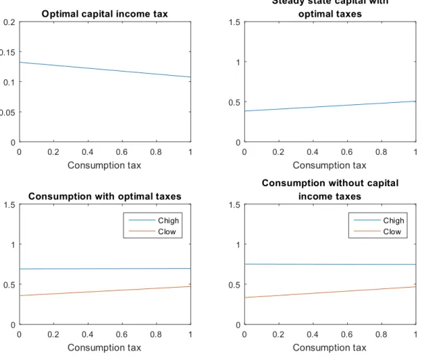
Firstly, we considered that in each period households were only subject to capital income shocks ( ). Given our simplifying assumption regarding the possible states of nature, we have that in each period households face either a positive capital income shock ( = ) or a negative capital income shock ( = ). In other words, the households’pre tax rate of return of capital can increase or decrease in each period. In …gures 1 and 2, we consider that is equal to 0.5.

Figure 1 illustrates the optimal taxation policy when households face only capital in-come risk. The optimal capital inin-come tax decreases as we increase the consumption tax.

(23)

of capital. This happens because there is a trade-o¤ between the capital income tax and the consumption tax. The purpose of the capital income tax in this model is to provide insurance against the idiosyncratic capital income risk, since it reduces the volatility in in-come and consequently the volatility in consumption. If we reduce the consumption tax we decrease the insurance capability of this …scal instrument. However, at the same time we are increasing the capital income tax, which can also be used as an instrument to diminish volatility in our stochastic model. However, using the capital income tax has a cost since it also a¤ects capital accumultation. Notice that although we vary the maximum consumption tax between 0 and 100%, the optimal capital income tax does not vary much.

0 0.2 0.4 0.6 0.8 1 Consumption tax 0 0.05 0.1 0.15

0.2 Optimal capital income tax

0 0.2 0.4 0.6 0.8 1 Consumption tax 0 0.5 1 1.5

Steady state capital with optimal taxes 0 0.2 0.4 0.6 0.8 1 Consumption tax 0 0.5 1

1.5 Consumption with optimal taxes

Chigh Clow 0 0.2 0.4 0.6 0.8 1 Consumption tax 0 0.5 1 1.5

Consumption without capital income taxes

Chigh Clow

Figure 1: Optimal consumption tax with capital income risk

(24)

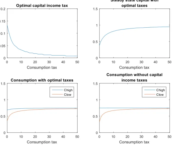
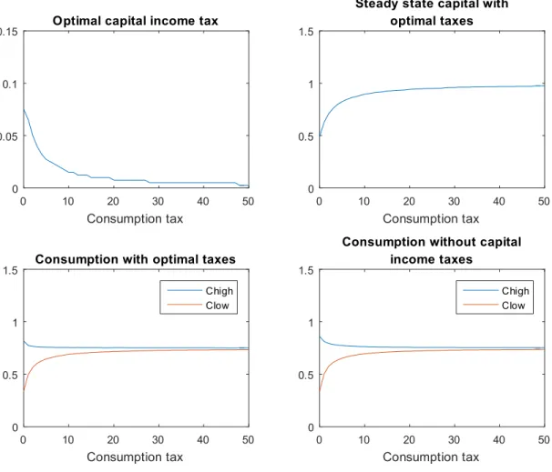
level of the consumption tax, the …rst best is attainable. As seen, the optimal taxation policy is not to tax capital and to tax consumption at an in…nitely large rate. However, we see that it takes an incredibly large consumption tax to reach our limit result. If this scenario was feasible, the steady state level of capital would converge to the …rst best level of capital, and the volatility of consumption would be fully eliminated. Thus, we would achieve the best possible welfare in our economy.

0 10 20 30 40 50 Consumption tax 0 0.05 0.1 0.15

0 10 20 30 40 50 Consumption tax 0 0.5 1 1.5

Steady state capital with optimal taxes 0 10 20 30 40 50 Consumption tax 0 0.5 1

Chigh Clow 0 10 20 30 40 50 Consumption tax 0 0.5 1 1.5

Chigh Clow

Figure 2: Optimal consumption tax with capital income risk, as the maximum consumption tax increases

(25)

6.3 Optimal taxation policy with only labor income risk

We now consider that households make their decisions in the presence of only labor income risk ("). In each period, households may be subject to a positive labor income shock (" = ) that results in an increase on their labor remuneration of , or they may face a negative labor income shock (" = ) that reduces their labor remuneration by . In the following graphical analysis we considered a equal to 0.5.

Figure 3 illustrates the optimal taxation policy in the presence of only labor income risk. The …rst result is that the capital income tax should be zero independently of the consumption tax. Since in our model the capital income tax was used as insurance against capital income shocks, it is reasonable that in this particular scenario it should be set to zero. 0 0.2 0.4 0.6 0.8 1 Consumption tax 0 0.05 0.1 0.15

0 0.2 0.4 0.6 0.8 1 Consumption tax 0 0.5 1 1.5

Chigh Clow

(26)

Furthermore, from the results of Section 5 we know that the households’decision over capital at the steady state level is not a¤ected by the consumption tax. This is veri…ed in the second frame, where we see that the steady state capital level is equal to the …rst best capital level. Even though the households’ decision regarding capital is not a¤ected by the consumption tax, this …scal instrument is relevant in this framework. Similarly to what happens in the presence of idiosyncratic capital income risk, the consumption tax can be used to reduce the volatility of consumption. In the bottom frames, we see that when the government increases the consumption tax the volatility of consumption decreases. The intuition is that in the good state of nature, when the households face positive labor income shocks, the government uses proportional consumption taxes to reduce consumption. In the bad state of nature, the government also taxes consumption, however there is a positive income e¤ect due to the lump-sum transfers that results in an overall increase in consumption. By increasing consumption when a household faces a negative labor income shock and decreasing consumption when a household is subject to a positive labor income shock, the consumption tax behaves once again as an insurance.

Figure 4 reinforces the results obtained in Section 5.1. Once more, we see that the optimal taxation policy in our economy is setting the capital income tax to zero and taxing consumption as much as possible. As the consumption tax rate converges to in…nity, we observe that the consumption in the good state of nature decreases signi…cantly and that the consumption in the bad state of nature increases exponentially. If it was feasible to apply such tax rates, the variability of consumption would be entirely suppressed and we would be in a …rst best situation.

(27)

0 10 20 30 40 50 Consumption tax 0 0.05 0.1 0.15

0 10 20 30 40 50 Consumption tax 0 0.5 1 1.5

Chigh Clow

Figure 4: Optimal consumption tax with labor income risk, as the maximum consumption tax increases

6.4 Optimal taxation policy with capital income risk and labor income risk

In this section, we will consider that households may be subject to both types of risk simultaneously. Furthermore, we will assume that the capital income shock and the labor income shock are correlated.

(28)

6.4.1 Negatively correlated capital income risk and labor income risk

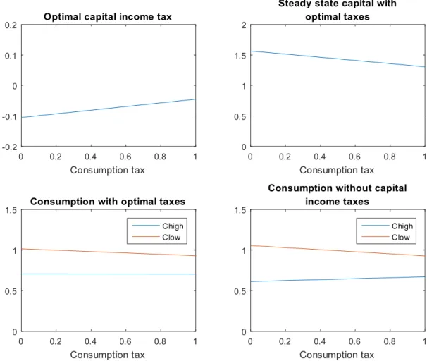
We start by considering a perfect negative correlation between the income shocks. We consider that in one state of nature a household faces a negative capital income shock ( = 0:2) and a positive labor income shock (" = 0:5), whereas in the other state of nature the household is subject to a positive capital income shock ( = 0:2) and a negative labor income shock (" = 0:5).

Figure 5 illustrastes the optimal taxation policy with capital and labor income risk when the magnitude of the labor shock is high. In this set up, we conclude that it is optimal to subsidize capital and that the subsidy decreases with the consumption tax.

0 0.2 0.4 0.6 0.8 1 Consumption tax -0.2 -0.1 0 0.1

0 0.2 0.4 0.6 0.8 1 Consumption tax 0 0.5 1 1.5 2

Chigh Clow

Figure 5: Optimal consumption tax with negatively correlated capital income risk and labor income risk

(29)

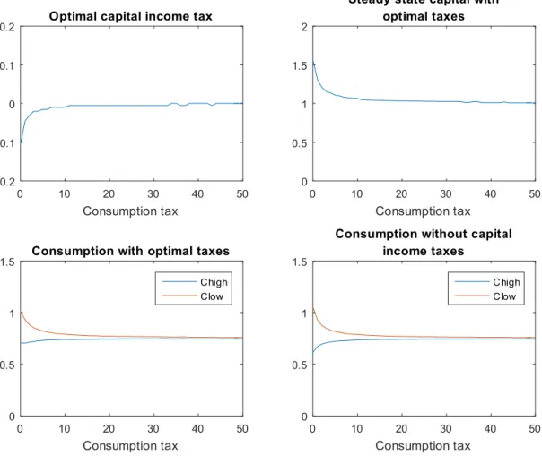
In Figure 6, analyze the optimal …scal policy in this set up as we increase the range of possible values for the consumption tax. We observe that if we use an in…nitely large consumption tax instead of subsidizing capital we eliminate the variability in consumption and the steady state level of capital converges to the …rst best level of capital.

0 10 20 30 40 50 Consumption tax -0.2 -0.1 0 0.1

0 10 20 30 40 50 Consumption tax 0 0.5 1 1.5 2

Chigh Clow

Figure 6: Optimal consumption tax with negatively correlated capital income risk and labor income risk, as the maximum consumption tax increases

6.4.2 Positively correlated capital income risk and labor income risk

We then considered a perfect positive correlation between the income shocks. In other words, we assumed that in one state of nature a household faces simultaneously a negative capital income shock ( = 0:3) and a negative labor income shock (" = 0:1), whereas

(30)

in the other state of nature the household is subject to a positive capital income shock ( = 0:3) and a positive labor income shock (" = 0:1).

0 0.2 0.4 0.6 0.8 1

Consumption tax

0 0.05 0.1

0 0.2 0.4 0.6 0.8 1 Consumption tax 0 0.5 1 1.5

Chigh Clow

Figure 7: Optimal consumption tax with positively correlated capital income risk and labor income risk

Figure 7 illustrates the optimal …scal policy in this set up. Firstly, we observe that the optimal capital income tax slightly decreases as we increase the consumption tax. This result is similar to the one obtained in Section 6.2. and the reasoning behind this result is the same, we use the consumption tax as a mean to reduce volatility so the role of the capital income tax as an insurance measure becomes less relevant. Furthermore, we observe that under this speci…cation of uncertainty consumption becomes less volatile as we increase the

(31)

an in…nitely large rate and to set the capital income tax to zero in order to fully eliminate the volatility in consumption and to reach the …rst best level of capital.

0 10 20 30 40 50

Consumption tax

0 0.05 0.1

0 10 20 30 40 50 Consumption tax 0 0.5 1 1.5

Chigh Clow

Figure 8: Optimal consumption tax with positively correlated capital income risk and labor income risk, as the maximum consumption tax increases

7 Concluding remarks

In this work we show that, even though the potential of consumption taxes is neglected at times, they can be powerful …scal instruments. In our set up, we provide an example of a stochastic model in which a tax on consumption can be used to provide insurance against capital income shocks and labor income shocks.

(32)

In the presence of idiosyncratic capital or labor income risk, we concluded that it is optimal to tax consumption at the highest rate possible. Given the reasonable levels for the consumption tax, we are not able to eliminate the capital income tax entirely. However, we are able to reduce the capital income tax which has a positive e¤ect on the steady state level of capital and on the welfare in our economy.

When households face a labor income shock, the capital income tax should be zero. But, uncertainty created by the labor income shocks can be signi…cantly reduced using consumption taxes. In the periods in which a household is subject to a positive labor income shock consumption tax is used to decrease the disposable income and consequently decrease consumption. On the other hand, when a household faces a negative labor income shock is able to smooth the e¤ect of this shock due to the lump sum transfers that result from the taxation of consumption of the other households.

In conclusion, in our stochastic neoclassical model the non state contingent consumption tax ful…lls the purpose of reducing the variability in the households’income, thus increasing the overall welfare in this economy.

References

[1] Aiyagari, S. Rao (1995) “Optimal Capital Income Taxation with Incomplete Markets, Borrowing Constraints, and Constant Discounting”, Journal of Political Economy 103, 1158-1175.

[2] Chamley, Christophe (1986) "Optimal Taxation of Capital Income in General Equilib-rium with In…nite Lives", Econometrica, 54, 607-622.

[3] Correia, Isabel H. (1996) “Should capital income be taxed in the steady state?”, Journal of Public Economics, 60, 147-151.

[4] Lucas, Robert E. (1990) “Supply-Side Economics: An Analytical Review”, Oxford Eco-nomic Papers, 42, 293-316.

[5] Panousi, Vasia and Reis, Catarina (2016) "A uni…ed framework for optimal taxation with undiversi…able risk", Working Paper.

(33)

8 Appendices

8.1 Numerical analysis

In this appendix, we derive the expressions that were needed to the perform the numerical analysis of the optimal taxation problem.

8.1.1 Expected value of consumption

We made the simplifying assumption that there were two states of nature to enable com-putations. Furthermore, in order to have the expected value of the shock capital income shock and the expected value of the labor income shock being both equal to zero (E( ) = 0 and E(") = 0), we assumed that each state of nature occurs with equal probability.

Then, we derived the expression for consumption in each state of nature and the expected consumption. From the individual resource constraint we know that the consumption of a household can be written as a function of the income shocks:

Ct( t; "t)(1 + ct) + Kt+1 ctE [Ct( t; "t)] = F (Kt; 1) + (1 )Kt+ "t+ (1 kt) tKt

C( ; ") = AK K + " + (1 k) K + cE [C( ; ")] 1 + c

Given our simplifying assumption, we are able to write the expected value of consump-tion as: E [C( ; ")] = 0:5Ch+ 0:5Cl E [C( ; ")] = 0:5 AK K + (1 k) K + cE [C( ; ")] 1 + c +0:5 AK K + (1 k) K + cE [C( ; ")] 1 + c

(34)

E [C( ; ")] = 0:5AK K 1 + c + 0:5AK K 1 + c + 0:5 + 0:5 1 + c + 0:5(1 k) K 0:5(1 k) K 1 + c + 0:5 cE [C( ; ")] + 0:5 cE [C( ; ")] 1 + c E [C( ; ")] = AK K 1 + c + cE [C( ; ")] 1 + c E [C( ; ")] 1 c 1 + c = AK K 1 + c E [C( ; ")] = AK K (17)

Finally, using equation (17) we obtain the following expressions for the consumption in the two states of nature:

Ch = C( ; ) = AK K + (1 k) K + cE [C( ; ")] 1 + c Ch= AK K + (1 k) K + c[AK K] 1 + c Ch = AK K 1 + c +(1 k) K 1 + c (18) Cl= C( ; ) = AK K + (1 k) K + cE [C( ; ")] 1 + c Cl= AK K + (1 k) K + c[AK K] 1 + c (1 k) K

(35)

8.1.2 Planner’s problem

We reach the optimal solution of the planner’s problem when the …rst order conditions with respect to the decision variables are veri…ed. Thus, we solved this problem by imposing that the derivatives of the Lagrangian with respect to the endogenous variables needed to be equal to zero.

Firstly, we set the …rst order condition with respect to the capital income tax ( k) to

zero and obtained an expression for the multiplier associated with the Euler equation ( ): @L @ k t+1 = 0 () t+1E _t+1( _t+1; "t+1) t+1Kt+1 t t E " u0 _C_t+1₍ t+1; "t+1) 1 + c_t+1 Fk(Kt+1; 1) + t+1 # = 0 () E u 0_{(C( ; "))} 1 + c [Fk(K; 1) + ] = E [ ( ; ") K] () E u 0_{(C( ; "))} 1 + c [Fk(K; 1) + ] = E [ ( ; ") K] () 0:5Ch + 0:5Cl 1 + c Fk(K; 1) + 0:5C_h 0:5C_l 1 + c = (0:5 _h K 0:5 _l K) () 0:5Ch_{1 +}+ 0:5Cl c AK 1+0:5Ch 0:5Cl 1 + c = K(0:5 _l 0:5 _h) () 0:5Ch_{1 +}+ 0:5Cl c AK 1+ 0:5Ch 0:5Cl 1 + c = 0:5 K Cl 1 + c 0:5 K C 1 l (1 + c)2 (1 k) AK 1 0:5 K Ch 1 + c + 0:5 K C 1 h (1 + c)2 (1 k) AK 1+

(36)

() 0:5Ch + 0:5Cl 1 + c AK 1+0:5Ch 0:5Cl 1 + c = 0:5 K Cl 1 + c C_h 1 + c 0:5 K C 1 l (1 + c)2 (1 k) AK 1 ! + 0:5 K C 1 h (1 + c)2 (1 k) AK 1+ ! () 2 6 6 6 6 6 6 6 6 4 0:5C_h + 0:5C_l 1 + c Fk(K; 1) + 0:5C_h 0:5C_l 1 + c +0:5 K C 1 l (1 + c)2 (1 k) AK 1 ! 0:5 K C 1 h (1 + c)2 (1 k) AK 1+ ! 3 7 7 7 7 7 7 7 7 5 = 0:5 K Cl 1 + c C_h 1 + c () = K Cl 1 + c C_h 1 + c 2 6 6 6 6 4 C_h + C_l 1 + c Fk(K; 1) + K C_l 1 (1 + c)2 (1 k) AK 1 ! +Ch Cl 1 + c K C 1 h (1 + c)2 (1 k) AK 1+ ! 3 7 7 7 7 5 (20)

Afterwards, since we know that the …rst order condition with respect to consumption also needs to be binding, we were able to derive an expression for the multiplier associated with the individual resource constraint as a function of the income shocks ( ( ; ")):

@L @Ct( t; "t) = 0 u0(Ct( t; "t)) = t( t; "t)(1 + ct) + t u00(Ct( t; "t)) 1 + c_t u00(C( ; "))

(37)

( ; ")(1 + c) = u0(C( ; ")) u00(C( ; ")) 1 + c + E u 00_{(C( ; "))} 1 + c + u 00_{(C( ; "))} 1 + c [(1 k) [Fk(K; 1) + ] ] ( ; ") = u 0_{(C( ; "))} 1 + c + u 00_{(C( ; "))} (1 + c)2 [(1 k) [Fk(K; 1) + ] ] ( ; ") = C 1 + c C 1 (1 + c)2 (1 k) AK 1+ (21)

From equation (21) we can derive the expression for the multiplier associated with each state of nature: h = ( ; ) = C_h 1 + c C_h 1 (1 + c)2 (1 k) AK 1+ (22) l= ( ; ) = C_l 1 + c C_l 1 (1 + c)2 (1 k) AK 1 (23)

Finally, using equations (22) and (23) we imposed that the …rst order condition with respect to capital needed to be binding:

@L @Kt+1 = 0 E [ _t( _t; "t)] = E h t+1( t+1; "t+1) h 1 + Fk(Kt+1; 1) + (1 kt+1) t+1 ii + _tE " u0 Ct+1( t+1; "t+1) 1 + c_t+1 1 k t+1 Fkk(Kt+1; 1) #

(38)

E [ ( ; ")] = E [ ( ; ") [1 + Fk(K; 1) + (1 k) ]] + E u 0_{(C( ; "))} 1 + c (1 k) Fkk(K; 1) [0:5 _h+ 0:5 _l] = 0:5 _h 1 + AK 1+ (1 k) + 0:5 _l 1 + AK 1 (1 k) + 0:5Ch + 0:5Cl 1 + c ( 1)AK 2(1 k) [ _h+ _l] = _h 1 + AK 1+ (1 k) (24) + _l 1 + AK 1 (1 k) + Ch + Cl 1 + c ( 1)AK 2(1 k)

In conclusion, after imposing that the …rst order conditions for the capital income tax ( k) and for consumption (Ct( t; "t)) were equal to zero, we found the optimal taxation