Improving malware detection with neuroevolution : a study with the semantic learning machine

i

Improving Malware Detection with

Neuroevolution: A Study with the Semantic

Learning Machine

Mário José Santos Teixeira

Project presented as partial requirement for obtaining the

Master’s degree in Business Intelligence and Knowledge

Management

ii

NOVA Information Management School

Instituto Superior de Estatística e Gestão de Informação

IMPROVING MALWARE DETECTION WITH NEUROEVOLUTION: A

STUDY WITH THE SEMANTIC LEARNING MACHINE

by

Mário José Santos Teixeira

Project presented as partial requirement for obtaining the Master’s degree in Business Intelligence, with a specialization in Knowledge Management and Business Intelligence

Advisor: Professor Ivo Gonçalves, PhD Co-Advisor: Professor Mauro Castelli, PhD

iii

ACKNOWLEDGMENTS

I would like to thank my supervisor Ivo Gonçalves for his guidance and support during this though challenge. Thank you also to my co-supervisor Mauro Castelli for his contribution, support and constant availability. For both of you to have properly introduced me into the world of Artificial Intelligence, with such a good and recent algorithm to work with, it was truly a great experience. A big thanks also to my mother, father and grandmother, who have always supported me throughout my whole academic life, pushing me to always do my best and really helped relieve me from other tasks so I could focus on my work.

A thank you to my work colleagues, that everyday incentivize me to be a better me and have always been very supportive to this project.

Last but definitively not least, to Bruna Ribeiro, that has been by my side through every single step of this hard journey, not letting me off the track for even a little bit, always giving me motivation and strength to continue, being my role model and a big part of this projects’ final result. A huge thank you.

iv

ABSTRACT

Machine learning has become more attractive over the years due to its remarkable adaptation and problem-solving abilities. Algorithms compete amongst each other to claim the best possible results for every problem, being one of the most valued characteristics their generalization ability.

A recently proposed methodology of Genetic Programming (GP), called Geometric Semantic Genetic Programming (GSGP), has seen its popularity rise over the last few years, achieving great results compared to other state-of-the-art algorithms, due to its remarkable feature of inducing a fitness landscape with no local optima solutions. To any supervised learning problem, where a metric is used as an error function, GSGP’s landscape will be unimodal, therefore allowing for genetic algorithms to behave much more efficiently and effectively.

Inspired by GSGP’s features, Gonçalves developed a new mutation operator to be applied to the Neural Networks (NN) domain, creating the Semantic Learning Machine (SLM). Despite GSGP’s good results already proven, there are still research opportunities for improvement, that need to be performed to empirically prove GSGP as a state-of-the-art framework.

In this case, the study focused on applying SLM to NNs with multiple hidden layers and compare its outputs to a very popular algorithm, Multilayer Perceptron (MLP), on a considerably large classification dataset about Android malware. Findings proved that SLM, sharing common parametrization with MLP, in order to have a fair comparison, is able to outperform it, with statistical significance.

KEYWORDS

Geometric semantic genetic programming; Artificial Neural Networks; Genetic Programming; Supervised Learning; Semantic Learning Machine; Multilayer Neural Networks

v

INDEX

1. Introduction ... 1

1.1. Background and Problem Definition ... 1

1.2. Study Objectives ... 2

1.3. Study Relevance and Importance ... 2

1.4. Structure ... 2

2. Literature Revision ... 3

2.1. Supervised Learning ... 3

2.2. Genetic programming ... 5

2.2.1. Individual representation ... 5

2.2.2. Initial population ... 7

2.2.3. Diversity operators ... 7

2.2.4. Fitness ... 9

2.2.5. Selection criteria ... 9

2.2.6. Implementation ... 10

2.3. Geometric Semantic Genetic Programming ... 11

2.3.1. Geometric semantic mutation ... 12

2.3.2. Geometric semantic crossover ... 13

2.4. Artificial Neural Networks ... 15

2.4.1. Biological neural networks ... 15

2.4.2. Learning ... 16

2.4.3. Network initialization ... 16

2.4.4. Hyper parameters ... 17

2.4.5. Other considerations ... 18

2.4.6. Gradient Descent ... 19

2.4.7. Backpropagation ... 19

2.4.8. Multilayer Perceptron ... 21

2.4.9. Evolutionary Neural Networks ... 24

2.5. Semantic Learning Machine ... 26

3. Methodology ... 30

3.1. Data ... 30

3.2. Algorithms ... 30

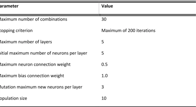
3.2.1. SLM configuration ... 31

vi

4. Results and analysis ... 35

4.1. First test ... 35

4.1.1. SLM variants ... 35

4.1.2. MLP variants ... 37

4.1.3. Overall comparison ... 41

4.2. Second Test ... 42

4.2.1. SLM variants ... 42

4.2.2. MLP variants ... 44

4.2.3. Overall comparison ... 47

5. Conclusions ... 48

6. Bibliography ... 49

LIST OF TABLES

Table 1 - SLM parameters ... 31

Table 2 - MLP parameters ... 34

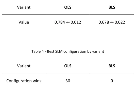
Table 3 - Validation AUROC for each SLM variant considered ... 35

Table 4 - Best SLM configuration by variant ... 35

Table 5 - Learning step for SLM-BLS ... 36

Table 6 - Number of iterations for each SLM variant considered ... 36

Table 7 - AUROC values for each MLP variant considered ... 37

Table 8 - Best MLP configuration by variant ... 37

Table 9 - Number of iterations for each MLP variant considered ... 37

Table 10 - Learning rate by MLP variant ... 38

Table 11 - L2 penalty by MLP variant ... 38

Table 12 - Activation functions use by MLP variant ... 38

Table 13 - Batch size by MLP variant ... 38

Table 14 - Batch shuffle use by MLP variant ... 39

Table 15 - Number of layers for each MLP variant considered ... 39

Table 16 - Total number of hidden neurons for each MLP variant considered ... 39

Table 17 - Momentum in MLP SGD ... 39

Table 18 – Nesterov’s momentum use in MLP SGD ... 40

Table 19 - Beta 1 in MLP Adam ... 40

vii

Table 21 - Validation AUROC for each SLM variant considered ... 42

Table 22 - Best SLM configuration by variant ... 42

Table 23 - Learning step for SLM-BLS ... 43

Table 24 - Number of iterations for each SLM variant considered ... 43

Table 25 - AUROC values for each MLP variant considered ... 44

Table 26 - Best MLP configuration by variant ... 44

Table 27 - Number of iterations for each MLP variant considered ... 44

Table 28 - Learning rate by MLP variant ... 44

Table 29 - L2 penalty by MLP variant ... 45

Table 30 - Activation functions use by MLP variant ... 45

Table 31 - Batch size by MLP variant ... 45

Table 32 - Batch shuffle use by MLP variant ... 45

Table 33 - Number of layers for each MLP variant considered ... 46

Table 34 - Total number of hidden neurons for each MLP variant considered ... 46

Table 35 - Momentum in MLP SGD ... 46

Table 36 – Nesterov’s momentum use in MLP SGD ... 46

Table 37 - Beta 1 in MLP Adam ... 46

Table 38 - Beta 2 in MLP Adam ... 46

LIST OF FIGURES

Figure 1 - Stoppage of training before starting to overfit (Henriques, Correia, & Tibúrcio, 2013)

... 4

Figure 2 - Simple GP individual represented as a syntax tree ... 6

Figure 3 - GP crossover diversity operator example ... 8

Figure 4 - GP mutation diversity operator example ... 8

Figure 5 - Genotype to semantic space mapping (Vanneschi, 2017) ... 12

Figure 6 – Biological Neuron (Karpathy, n.d.) ... 15

Figure 7 – Perceptron (Dukor, 2018) ... 16

Figure 8 - Simplest form of a multilayered artificial neural network ... 26

Figure 9 - SLM Mutation (Gonçalves, 2016) ... 27

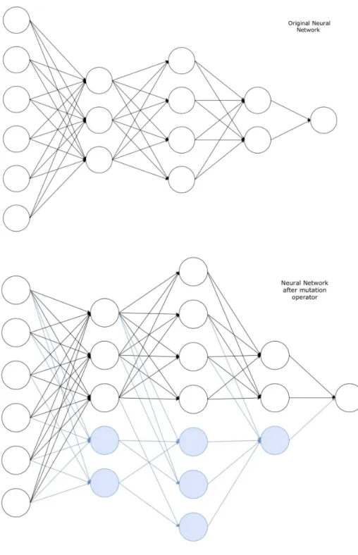
Figure 10 - Multilayer SLM mutation operator example ... 33

viii

Figure 12 - Boxplots respective to the second test for the AUROC values of SLM and MLP

algorithms respectively ... 47

ix

LIST OF ACRONYMS AND ABBREVIATIONS

GSGP Geometric Semantic Genetic Programming

GP Genetic Programming

ANN Artificial Neural Network

EANN Evolutionary Artificial Neural Network

SLM Semantic Learning Machine

1

1. INTRODUCTION

This chapter’s goal is to provide the reader an introduction of this study’s work, clarifying its background and the motivation and relevance that led to its development, as well as the objectives and structure of this work.

1.1. B

P

D

Machine Learning statistical methods and algorithms go as early as the 1950’s decade, with a continual growth of evolution throughout the years. A particular goal for these systems is to output intelligence comparable to the output a human being would be able to give, being therefore new human-competitive systems (Gonçalves, 2016; Koza, Keane, & Streeter, 2003; Turing, 1950).

A big focus on this topic has been the development of systems capable of self-sustainability and continual improvement, such as evolutionary artificial neural networks (Yao, 1993, 1999). The continuous aim on this topic has been to replicate as closely as possible the behavior of biological neural networks that, based on several distinct biological sensorial inputs, generate specific knowledge from it. On this particular subject, machine learning refers to the task of generating knowledge (predictive patterns) based on a set of examples of unseen data. The maintenance for these systems is to keep being fed data in order to have more distinct training cases, to better assess and perfect the evaluation model that generates the predictive output, avoiding the typical challenge of overfitting in order to be successful.

A specific topic on this subject is Genetic Programming (GP) algorithms that are a class of computational methods inspired by natural evolution, having the great characteristic of flexibility on model’s evolution, having no a priori constrains that could restrict the set of functions or structure to be used. The downside of GP is the constant concern on overfitting (Gonçalves, 2016; Gonçalves, Silva, & Fonseca, 2015a).

The system in focus on this study, Geometric Semantic Genetic Programming (GSGP), is a recently proposed strand of GP focused on smoothing the fitness landscape as unimodal (no local optima solutions) with a linear slope, which allows for an easier search of the semantic space. This characteristic can be applied to any variation of supervised learning task, with great results when compared to other learning algorithms while still having already evidence of not falling into the overfitting problems of standard GP (Gonçalves et al., 2015a; Moraglio, Krawiec, & Johnson, 2012; Vanneschi, 2017).

Gonçalves studied the application of GSGP to artificial neural networks, creating the Semantic Learning Machine (Gonçalves, 2016; Gonçalves, Silva, & Fonseca, 2015b). All recent studies to test SLM have proven that it can outperform state of the art evolutionary algorithms as well as classic algorithms on several distinct benchmark tasks (Gonçalves et al., 2015b; Jagusch, Gonçalves, & Castelli, 2018). The aim of this project is to expand the knowledge on SLM’s competitive ability, implementing it on multilayer neural networks and testing how it will perform against the well-established Multilayer Perceptron (MLP) algorithms on large datasets.

2

1.2. S

O

The scope for this project is to implement the SLM algorithm on neural networks with multiple hidden layers. Afterwards, it will be put to the test on a large dataset and compare its results against MLP’s results on the same dataset.

In pursuance of this project’s vision, the following objectives have been defined:

1. Evaluate the state of art on artificial neural network algorithms, focusing on MLP 2. Define common parameters for SLM and MLP for a fair comparison

3. Implement the SLM model containing GSGP algorithm and expand it to neural networks with multiple hidden layers

4. Implement a popular MLP algorithm

5. Test both algorithm’s performance against the same dataset 6. Compare results and analyze conclusions

1.3. S

R

I

The proposed project implementation has impact on the fields of Genetic Programming, Geometric Semantic Genetic Programming, Artificial Neural Networks and Semantic Learning Machine. GSGP and SLM has already proven themselves with some interesting results on other study applications (Castelli, Vanneschi, & Silva, 2014; Gonçalves et al., 2015b; Jagusch et al., 2018; Vanneschi, 2017) by outperforming traditional genetic programming algorithms. There are still areas of study that need to be assessed for GSGP to be considered a state of art. One of them is the lack of evidence on multi-layered neural networks (Gonçalves, 2016).

The expected outcome is for SLM to have consistently better accuracy on the results versus MLP. If successful, the results would reinforce that GSGP is capable of being applied to any artificial learning system of any kind of complexity, proving its ability of generalization. This would also mean that even for more complex artificial learning systems, there would not be a need for the concept of population and convergence operators such as crossover. This will also allow for more opportunities for proof of concepts for this approach in comparison to other fields of study.

1.4. S

This chapter intends to guide the reader, detailing the structure for this document.

Alongside this chapter, the document is composed of 6 chapters. Chapter 2 contains the literature background required for the reader to be contextualized and integrated with previously existing studies. Chapter 3 details the methodology used to obtain the results. Chapter 4 presents and analyzes the results obtained. Chapter 5 summarizes the key points to retain from this study. Chapter 6 presents the bibliography used.

3

2. LITERATURE REVISION

2.1. S

L

Supervised learning comprehends a machine learning task in which, for a given set of instances, a model should be able to build an algorithm capable of understanding the pattern that the input instances represent, in order to be able to predict any future unseen instance as precisely and accurately as possible (Gonçalves, 2016). These features not only aim to complement knowledge where humans cannot extract alone from direct data analysis, but also provide other means of comparison, validation of results, and a more accurate version of outcomes when referring to prediction tasks based on relation between multiple variables (Kotsiantis, 2007).

The training is supervised, meaning that all input data is represented by the same features and also that every instance has an assigned target value. The dataset is a collection of labelled vectors {(𝑥$, 𝑦$)}$)*+ , in which each dimension 𝑗 = 1, … , 𝐷 contains a value that is part of the description of

the example, also named as feature. All features 𝑥1 _{should translate the same knowledge about the}

𝑥₂, for all 𝑥2, 𝑘 = 1, … , 𝑁 on the dataset. Label 𝑦$ can either be an element of a set of classes

{1,2, … , 𝐶} or a real number (Burkov, 2018). The model’s algorithm aims at being capable of inferring a function that reflects the underlying pattern behind the variables to obtain the predicted outcome, with the least deviation possible from the actual target. The relation pattern of the features in comparison to the target variable is the learning goal of the algorithm (Cunningham, Cord, & Delany, 2016).

Depending on the type of prediction, different learning tasks can be defined. For a numerical value problem, a regression task is assigned, while when trying to label the instance to a given set, a classification task is preferred. The case when the target varies between two values is referred to as binary classification (Gonçalves, 2016; Kotsiantis, 2007).

Since the goal of the model will be to predict unidentified individuals, another crucial aspect to consider when producing the model is its generalization ability. The generalization of a model reflects its accuracy when applied to unseen data. If the full dataset was provided for the model to train upon, the end result would be an algorithm perfectly shaped to that particular input dataset, but with a poor prediction power for new unseen instances. The main goal of a model is to have the best result possible on the prediction of unseen data, in other words, having a good generalization ability. Therefore, a supervised learning model should have the best generalization ability possible (Gonçalves, 2016). Since supervised learning can be implemented to countless scopes, each has its own metrics and performance priority preferences. Due to this, sometimes trade-offs are inevitable, and the error metrics also vary according to the applied domain, being possibly even biased by it (Cunningham et al., 2016). For this reason, it has been proven that the same algorithm performs differently according to its parametrization, which can lead to models excelling on some metrics but failing the threshold of others. Some of the best overall performing predictors, according to benchmark tests, are Bagged Trees, Random Forests and Neural Networks (Caruana & Niculescu-Mizil, 2006).

In order to improve the generalization ability of the model, the provided dataset is usually split into two different sets. The first one, the training dataset, will be used to train and evolve the model. From here, the algorithm should already be able to infer a relation between the input features. The second

4 set, referred to as the testing dataset, will be used to evaluate the performance of the model on unseen data and therefore understand the generalization ability of the algorithm. A model should aim to perform well in test data as it translates on good performance upon future unseen data. However, models may output better results on training data than on unseen data. Such models are said to be overfitting, translated to an exaggerated modulation to the pattern of the training data. Learning the algorithm to predict the training data is useless on the overall scheme since, as previously mentioned, the aim is to fit the model to unseen data (Gonçalves, 2016). Figure 1 shows how the testing set can be used to stop training before it starts overfitting.

5

2.2. G

Genetic programming (GP) (Koza, 1992) is an extension of the genetic algorithms (GA) theoretical approaches, dealing with GA’s representation limitations by applying them to dynamically flexible structures of computer programs. Therefore, as well as GA, GP mimics its premises on the principles of biological processes that nature has perfected over the years. Nature’s structures have evolved over long periods of time as a consequence of Darwin’s natural selection as well as of extremely rare random genetic mutations (Banzhaf, Martín-Palma, & Banzhaf, 2013). In nature, those same structures would be put to test up against the environment, on which the fittest to it would be the ones to survive for further generations, creating a new population. Keeping the same mindset, originated the drive to understand how could computer programs evolve by themselves and assure a better result on each generation (Angeline, 1994; Krawiec, Moraglio, Hu, Etaner-Uyar, & Hu, 2013).

The most frequently used GP representation explains the computer programs as trees, known as standard GP, but there also exist other representations such as linear GP and graph GP. Standard GP consists on nodes, that can be either functions or input, further explained below, connected amongst themselves by branches (Fan, Gordon, & Pathak, 2005; Gonçalves, 2016; Krawiec et al., 2013).

The process itself remains fairly similar to nature’s approach and also to the genetic algorithm’s one, which in the case of computer programs, the goal is to evolve an algorithm up to a solution that has the best results possible. Let a computer program solution be named onwards as individual. The best individual would be the one that best represents the solution that is closest to the optimal one. All the individuals pass through an evaluation as a way to understand how well each one performs solving the task at hand, being then assigned a correspondent value. In order for an individual to be considered better than another, a performance measure must be defined, related to the problem under analysis, being that measure named fitness. In GP, due to the selective pressure, the fittest individuals will be the ones to reproduce into the next generation. The individual with the highest fitness is the one with the least distance from the optimal solution and therefore is considered to be the best individual (Fan et al., 2005; Krawiec et al., 2013).

2.2.1. Individual representation

In GP, an individual represents a computer program. There have been several distinct representations proposed by researchers, such as the cartesian (Miller, 1999), linear (Banzhaf, 1993) and, the one that fits the purpose of this project, syntax trees (Koza, 1992). Figure 2 displays a simple GP individual represented as a syntax tree.

6

Figure 2 - Simple GP individual represented as a syntax tree

There are two sets of components on a syntax tree: nodes and leaves. Nodes are populated from a existing function set, while the leaves, also known as terminals, can be set based on an also pre-existing terminal set. All individuals will be built based on the same function set and terminal set, meaning that the creation of these two defines the boundaries on how GP programs can be generated (Koza, 1992; Poli, Langdon, McPhee, & Koza, 2008).

The function set 𝐹 = {𝑓*, 𝑓9, … , 𝑓:} contains all possible operational functions to be used by the

program. These can be logical functions (AND, OR, NOT, IF, etc.) or mathematical (+, -, *, sin, cos, etc.) (Koza, 1992). Koza also defined an important property, named closure, meant to keep the programs’ integrity. This assures the programs’ safety by avoiding forbidden operations, such as the division by 0, that was replaced by safe division, which returns 1 when encountering a division by 0. It also maintains the program’s functionally by ensuring a type consistency, for instance, avoiding mixing the sum of a mathematical terminal with a Boolean result (Koza, 1992).

The terminal set 𝑇 = {𝑇1, 𝑇2, … , 𝑇𝑁} contains the program’s available arguments. These can be the program’s input variable, possible constant values or even random values.

Taking into consideration the individual in Figure 2, one can understand it was built with, at least, function set 𝐹 = {+,∗} and 𝑇 = {𝑥, 𝑦, 1} .

7

2.2.2. Initial population

At the start of the evolution process, a new population of individuals is created. The number of individuals created depends on the parametrization given to the specific GP program. Upon creation of the population, the following parametrization is shared by all individuals:

• Function set (F) - which are the available functions for individuals to use;

• Terminal set (T) - all the input variables and constants that are added when there is enough knowledge on the problem to do so;

• Depth (d)- determines how many levels shall an individual have at maximum.

There are three possible methods to create new individuals. The first, the full growth method, sees an individual to be created with maximum depth level on all the possible branches of the tree, generating a tree with 2𝑑 – 1 nodes total. The second way to create individuals is the growth method, that, at each tree level, randomly selects if the node will be a terminal or a function, until depth 𝑑 – 1, to which afterwards all nodes are considered as terminals. The third and final growth method is called ramped half-and-half, which initializes half of the population by using the full method and the other half with the growth method (Koza, 1992).

2.2.3. Diversity operators

GP has at its disposal two operators to be applied to individuals, to create some genetic diversity amongst the population, and hopefully create better and more robust individuals. The operators are crossover and mutation, both needing individuals from an existing population, denominated as parents, producing the same number of new individuals, called children or offsprings. Both operators may be applied depending on a probability assigned for each one, but not at the same time (Koza, 1992; Krawiec et al., 2013; Poli et al., 2008). Commonly, crossover is applied with higher frequency than mutation (Gonçalves, 2016).

2.2.3.1. Crossover

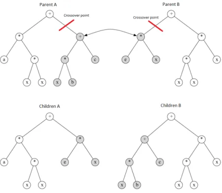
The crossover operator requires two parents from the existing population and produces two children. It randomly selects two different nodes (one from each parent) known as crossover points and, subsequently, it swaps the subtrees rooted at the selected crossover points. Subtree from parent A is added to parent B at its crossover point, producing the first children. The symmetrical process is then applied again to get the second children. These new structures will be the two new children of the current generation (Gonçalves, 2016; Koza, 1992). Figure 3 illustrates this procedure.

8

Figure 3 - GP crossover diversity operator example

2.2.3.2. Mutation

The mutation operator requires only one parent. It is intended to allow for random diversity to be induced in the population (Koza, 1992). A random point on the tree is selected, called mutation point. A random tree is then generated and the subtree from the parent is cut off, to be replaced by the new random tree. The new structure will be the offspring to be included in the current generation (Gonçalves, 2016). Figure 4 illustrates the mutation procedure.

9

2.2.4. Fitness

The fitness of an individual is not directly tied to it. It is merely a representation of that individual’s quality over a specific set of data. This allows different individuals to be compared amongst each other, when presented to the same set of data, under the same fitness evaluation measure, named the fitness function. The closest an individual gets from correctly evaluating a set of input instances according to their respective targets, the higher fitness value that individual has (Koza, 1992).

A very common fitness function is the Root Mean Square Error (RMSE), also applied to this study’s tests. Its goal is to evaluate the overall distance from all the computed outputs upon comparison to their targets. Being 𝑦$ the computed output for observation 𝑖 and 𝑦B$ its actual target, RMSE is:

𝑅𝑀𝑆𝐸 = G∑:$)*(𝑦B$− 𝑦$)9 𝑛

2.2.5. Selection criteria

Through fitness evaluation of individuals, it is possible to compare them and rank them by fitness value. The best-ranked individuals will be used to evolve the population, while the worst ones are discarded. All individuals have an attached probability of being selected for future generations, falling the choice on the selection criterion applied.

Different approaches can be taken when considering, first, which individuals will be chosen as parents to apply the diversity operators to and, second, which population should carry on evolving into the next generations. One method of selection is using Tournament Selection, that randomly groups a certain number of individuals with uniform probability and the best one is selected according to its fitness output. The survivor selection is used as well, being the most common method the elitist survival, to which only the best individuals are kept going further into next generations. Several precautions need to be taken into consideration when parametrizing the selection criteria. Keeping only the best individual might convert the solution into a local optima one. Keeping too many individuals and the search process is heavier and more sparse space, to which usually new offsprings get better results on. Parametrizing on a balanced search is a key aspect to be taken into consideration (Gonçalves, 2016; Krawiec et al., 2013).

10

2.2.6. Implementation

To implement GP, one must define distinct parameters as Koza suggested (Koza, 1992): • Function set

• Terminal set

• Fitness evaluation function • Population initialization method • Maximum tree depth (optional) • Selection operator

• Crossover probability • Mutation probability • Stopping criterion

It should be noted that some parameters require additional parametrization. For instance, if Tournament Selection is the chosen selection operator, the number of individuals to be considered for the Tournament should also be defined.

After defining these, the algorithm works by: 1. Initializing the population

2. While the stopping criterion is not met: 1. Evaluate all the individual’s fitness 2. Apply selection operator

3. For each new individual to be created:

1. Calculate what diversity operator will be applied 2. Choose the parent

3. Apply the diversity operator 4. Replace the population with a new one 3. The best individual of all will be the final solution

It should also be noted that, due to GP’s main goal of freely exploring the search space, it is possible that even with the same parametrization, two GP programs might produce different end results.

11

2.3. G

S

G

P

In 2012, genetic operators for GP were introduced, denominated as geometric semantic operators, whose main feature of interest was the induction of a fitness landscape characterized by the absence of locally sub-optimal solutions (unimodal fitness landscape), for any supervised learning problem where the program’s fitness is a distance between a set of target values and the corresponding set of calculated outputs (Gonçalves, Silva, Fonseca, & Castelli, 2016; Moraglio et al., 2012; Vanneschi, 2017). The semantics of a program is defined as the mathematical function to which afterwards corresponds a respective fitness output, when applied to an input vector of data. The n-dimensional space to which the vector belongs to is denominated as semantic space. The target vector itself is a point in the semantic space (Figure 5) (Vanneschi, 2017). Traditional GP operators act on the syntactic representation of individuals, their genotype, ignoring their actual significance in terms of semantic value. Moraglio et. al. question if such a semantically apathetic evolution would fit well across problems from different domains, since the meaning of the problems determines their search success (Moraglio et al., 2012).

Although these new semantically aware methods outputted with greater performance than traditional methods, they had the drawbacks of being very wasteful since they were focused on a trial-and-error approach and also that they do not provide insight on how syntactic and semantic searches relate to each other (Moraglio et al., 2012).

Moraglio et al. proposed a formal implementation of these semantically aware operators of GP, named Geometric Semantic Genetic Programming (GSGP) (Moraglio et al., 2012). GSGP has a great advantage in terms of evolvability, given by a unimodal fitness landscape. One limitation that persists is the task of visualizing and understanding the final solution generated. Not having any locally sub-optimal solution makes any symbolic regression easy to optimize for GP, regardless of the size of data. This eliminates one of the GP limitations of being extremely difficult to study in terms of fitness landscapes, due to the extreme complexity of the genotype/phenotype mapping and also the complexity of the neighbourhoods induced by GP crossover and mutation. The characteristic of having a unimodal error surface is quite rare on machine learning and should give GP a clear advantage compared to other systems, at least in terms of evolvability (Gonçalves, 2016; Moraglio et al., 2012; Vanneschi, 2017; Vanneschi, Castelli, Manzoni, & Silva, 2013).

12

Figure 5 - Genotype to semantic space mapping (Vanneschi, 2017)

2.3.1. Geometric semantic mutation

The objective of the Geometric Semantic Mutation (GSM) is to generate a transformation on the syntax of GP individuals that has the same effect as the box mutation (Gonçalves et al., 2015a; Vanneschi, 2017). GSM always has the possibility of creating an individual whose semantics is closer to the target than before. The definition (Moraglio et al., 2012) is:

Definition – Given a parent function 𝑃: 𝑅: _{→ 𝑅, the geometric semantic mutation with mutation step}

ms returns the real function 𝑃𝑀 = 𝑃 + 𝑚𝑠 . (𝑇Q* – 𝑇Q9), where 𝑇Q* and 𝑇Q9 are random real

functions.

Each element of the semantic vector of PM is a slight variation of the corresponding element in P’s semantics. The variation is of small proportion since it is given by a random expression centered in zero. By changing the mutation step ms we are able to tune the impact of the mutation.

In order to make the perturbation even weaker, it is useful to limit the codomain of the possible outputs of the random trees into a given predefined range. This allows for a better control of the mutation. To guarantee that the output of the random trees assume values in [0,1], it is possible to use the output of a random tree as the input of a logistic function (Vanneschi, 2017).

The importance of having random individuals included in the mutation instead of random numbers is that when an individual is mutated, the aim is to perturb each one of its coordinates by a different amount. The perturbation must have the following properties (1) it has to be random; (2) it has to be likely to be different for each coordinate; (3) it does not have to use any information from the dataset. A random expression is likely to have different output values for different fitness cases. The difference between two expressions is used instead of just one random expression because, it may happen that, especially in the final part of a GP run, some of the coordinates have already been approximated in a satisfactory way, while others have not and in that case, it would be useful to have the possibility of

13 modifying some coordinates and not modifying others. The difference between two random expressions is a random expression centered in zero. By using the difference between two random expressions we are imposing that some coordinates may have a perturbation likely to be equal, or at least as close as possible, to zero (Gonçalves et al., 2015a; Moraglio et al., 2012; Vanneschi, 2017; Vanneschi et al., 2013).

2.3.2. Geometric semantic crossover

Geometric crossover generates one offspring that, for each coordinate I, a linear combination of the corresponding coordinates of the parents p and q, with coefficients included in [0,1], whose sum is equal to 1.

oi = (ai * pi) + (bi*qi)

where ai ∈ [0,1], bi ∈ [0,1] and ai + bi = 1

The offspring can geometrically be represented as a point that stands in the segment joining the parents. The objective is to generate a tree structure that stands in the segment joining the semantics of the parents. The definition states (Moraglio et al., 2012):

Definition – Given two parent functions 𝑇*, 𝑇9: ℝ:→ ℝ, the geometric semantic crossover returns the

real function 𝑇TU = (𝑇* . 𝑇Q) + ((1 − 𝑇Q) . 𝑇9), where 𝑇Q is a random real function whose output

values range in the interval [0,1].

Using a random expression TR instead of a random number can be interpreted analogously as the same

as to Geometric Semantic Mutation. For the geometric crossover, the fitness function is supposed to be measured with the Manhattan distance; if the Euclidean distance is used instead, then TR should be a random constant instead (Moraglio et al., 2012; Vanneschi, 2017).

Since the offspring 𝑇TU stands between the semantics of both parents 𝑇* and 𝑇9, it cannot be worse

than the worst of its parents.

Geometric semantic operators create offsprings that contain the complete structure of parents plus one or more random trees, therefore the size of the offspring is always much larger than the size of their parents. To respond to this issue, an automatic simplification after each generation, on which the individuals are replaced by semantically equivalent ones, was suggested (Moraglio et al., 2012). This, however, increases the computational cost of GP and is only a partial solution to the growth. Automatic simplification can also be a very hard task.

Another implementation was originally presented assuming a tree-based representation (Castelli, Silva, & Vanneschi, 2015; Vanneschi et al., 2013) but can actually fit any type of representation. This algorithm is based on the idea that an individual can be fully described by its semantics. At every

14 generation, a main table containing the best individuals is updated with the semantics of new individuals and the information needed to build new ones is saved. In terms of computational time, the process of updating the table is very efficient as it does not require the evaluation of the entire trees. Evaluating each individual requires constant time, independent from the size of the individual itself. There is also a linear space and time complexity with respect to population size and number of generations. The final step of this implementation is the reconstruction of the individuals, focusing only on the final best one. Disregarding the time to build and simplify the best individual, which can be made offline after the algorithm runs, the proposed implementation allowed to evolve populations for thousands of iterations with a considerable speed up with respect to standard GP (Gonçalves, 2016; Gonçalves et al., 2015a; Vanneschi, 2017).

15

2.4. A

N

N

With the continuous developments on artificial intelligence, scientists/investigators decided to study and find a way to mimic the human brain, dating the first experiences as far as 1943 (McCulloch & Pitts, 1943). Artificial Neural Networks (ANN) are machine learning models that intend to replicate the human brain’s operational behaviour. They are extremely powerful due to their non-linear interpolation ability as well as the fact that they are universal approximators, all of this while being completely data driven. Three elements are particularly important in any model of artificial neural networks: structure of the nodes; topology of the network and the learning algorithm used to find the weights (Buscema et al., 2018; Haykin, 2004; Raul Rojas, 1996). ANNs are usually used for regression and classification problems such as pattern recognition, forecasting, and data comprehension (Gershenson, 2003).

2.4.1. Biological neural networks

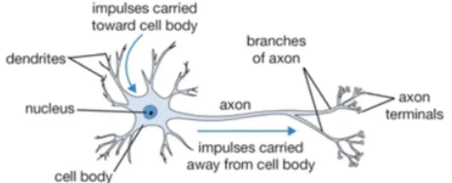
The information flow of the human brain happens via form of neurons, approximately 100 billions of them (Herculano-Houzel, 2009), forming extremely complex neural networks. Each neuron, as the one represented on Figure 6, is composed by the dendrites that receive ions through electrical stimuli called synapses. All the synapses flow into the neuron cell body, denominated as nucleus, responsible for processing the input signal. Via the neuron’s axon, all the synapses’ ‘information’ is propagated to its neighbours, depending only on the strength of the connection and sensitiveness to the signal. The axon terminals of a neuron are connected to its neighbours’ dendrites. Researchers conservatively estimate there are more than 500 trillion connections between neurons in the human brain. Even the largest artificial neural networks today don't even come close to approaching this number (Patterson & Gibson, 2017).

Figure 6 – Biological Neuron (Karpathy, n.d.)

ANNs reflect the exact same behaviour. Each ANN is represented by neurons and their connections to each other. To the connection between neurons are associated weights. ANNs are also split by layers, in order to dictate an information flow. Neurons of one layer communicate only with the neurons of the next layer, and to each connection a weight is assigned. There is no communication between neurons that belong to the same layer. The minimum structure of an ANN must contain one input layer and one output layer. In between, more layers can be added to the structure, being those layers denominated as hidden layers. Each ANN can contain between zero and infinite hidden layers.

16 The simplest form of an ANN is called the perceptron (Figure 7), which is represented by containing merely one layer of input neurons connected to a single output neuron. The number of neurons of the first layer, denominated as input layer, will be the same as the number of variables of the problem to which the neural network is being applied to and the value for each one of these neurons is the value of each variable. The value of each input neuron is then multiplied to the assigned weight between that neuron and the neuron of the next layer. The result of the output neuron is the sum of all input neurons times their weights. To the calculated value, a transfer function called activation function is applied, making all results that are brought into the network have an output that can be split by a linear function. Therefore, a limitation of the Perceptron is that it can only be applied to linearly separable problems (Gershenson, 2003; Gonçalves, 2016; Raul Rojas, 1996; Yao, 1999).

Figure 7 – Perceptron (Dukor, 2018)

2.4.2. Learning

The process of implementation of a neural network includes two phases: learning and testing. To define how can the neural network learn, a definition of learning must be set. Everyday learning can be translated into an increase of knowledge on a subject by means of studying, experience or being taught. Comparing this concept with what was described above as Supervised Learning, the learning process of neural networks is the ability to optimize either its weight values or structure, so that with the input values it takes, based on the difference of the network’s output compared to the actual value, it can optimize itself to produce the lesser error possible, which translates to better results. The testing refers to the application of the model built (Gonçalves, 2016).

2.4.3. Network initialization

The topology of an ANN references its external structure, stating the layers, the neurons and the connections between them. Its configuration can determine the success or failure of the model. However, there are no pre-determined rules to define it. Different types of ANNs will have different

17 topologies, however best the specialists responsible for the experiment find fit to be applied to it. It can have between a single layer up to a large number of them. For instance, the multilayer perceptron (MLP) is a standard multilayer feed forward network (the calculation between neurons is feed forward from the input nodes to the output nodes) with one input layer, one output layer, and one or multiple hidden layers. Because of the importance of the topology, it would make sense to use a GA to determine it, but researches showed it does not give better results (Yao, 1993).

All of these decisions influence the ANNs performance. However, the most efficient way is still to have an expert on both ANNs as well as the problem at hand to initialize them, as there is no scientific way of automatic optimization. These choices involve not only all of the ANNs hyperparameters, but others relevant to the learning process such as population size, number of generations, probability of crossover and mutation operations and what the best selection method is if an evolutionary training approach is considered (Buscema et al., 2018; Gershenson, 2003; Yao, 1999).

2.4.4. Hyper parameters

ANNs, as mentioned on the chapter above, are distinguished from each other based on their parametrization. Topology wise, there have already been mentions to the number of hidden layers of a network as well as the number of hidden neurons on each layer, again, not existing a scientific approach to assign values to these two.

Apart from those parameters, there are other tuning parameters that heavily affect the final outcome. First of those is the decision when to stop training the neural network and to those we name the stopping criterion. These can vary between knowledge specific suggestions, such as to stop training when the output reaches a certain threshold, to mathematical as the error deviation variation criteria, that takes into account how much the error differs from one training epoch to the other. There are also other options more generic, as stopping training after a certain amount of time, after a certain number of training epochs or if there is no improvement after a defined number of training epochs. Another very important parameter is the learning rate (or also known as learning step), that controls the “navigation” of the neural network within the fitness landscape. A high learning step sets a high variability on the results, since it will always try to compensate the gap between the target values and the current output with a high correction. A low learning step might make the ANN stuck on a local minimum on the fitness landscape as well as increase the processing time. A general good approach is to have a relatively high learning step at first and decrease it after each training epoch. Other experiments have tried setting different rates for different layers (Haykin, 2004; Srinivas, Subramanya, & Babu, 2016).

Another part of Neural Network’s optimization decisions is the choice of the activation functions. These are particularly useful to induce non-linearity to the model, a key aspect on their universal approximator ability. Apart from this, different activation functions come with different perks. The vastly most used are the sigmoid function, squashing values between 0 and 1, tangent function that tends to center the output to 0 which has an effect of better learning on the subsequent layers, also with negative and positive output values considered as 0 and 1 respectively and finally one that is drawing a lot of interest which is the ReLU function, which removes the problem of vanishing gradient

18 faced by the above two (i.e. gradient tends to 0 as x tends to +infinity or -infinity). ReLU has the disadvantage of having dead neurons which result in larger NN's without an associated benefit. All the neurons on the network except the input layer one’s should have an activation function being applied to them (Gershenson, 2003).

The number of neurons on the output layer is dependent on the specific case being studied. In case the final output is binary, either one value or another, or the target is a continuous number, a single output neuron is required. In case there are three or more output classes, an output neuron must be created for each target class and each instance should have only one of those output neurons set to 1 (Buscema et al., 2018).

2.4.5. Other considerations

Even if they are to be considered irrelevant when compared to their trade-off, a few drawbacks still need to be considered on ANNs. If not properly parametrized or when data contains noise, the resulting ANN can become excessively complex compared with statistical techniques in some scenarios. Another big common critique relates to its interpretability, since they work like black-boxes. Some intermediary determinations are meaningless to humans and the final result is in most of the cases unable to be explained in human terms. In cases of improper parameter tuning can also make the ANN unable to achieve reasonable results, as, for instance, a learning rate too high can result a high fluctuation on the search space, making the ANN unable to land on a local or global optimum. Some of these downsides can be solved by making an adjustment in the ANN using gradient descent or genetic algorithms, applying them to determine the connection weights, the network topology or even defining the learning rules. These ANNs are considered innovative and the literature about them is still relatively poor (Priddy & Keller, 2009; Srinivas et al., 2016; Yao, 1999).

19

2.4.6. Gradient Descent

A simple iteration of any kind of neural network bases itself on taking the data through the input layers, propagating it onward to the neurons on the hidden layers and getting a final output, which is then compared to the actual target to measure the accuracy of the model. The behavior of the network from the moment the first iteration ends until the end of training is what usually characterizes it (Rumelhart, Hinton, & Williams, 2013).

The most common, and with better results shown, ANNs are those whose weights are randomly generated on the beginning of the training process and are then iteratively updated at the end of each learning iteration. The most common methods to achieve this are gradient descent methods, such as backpropagation, simulated annealing or genetic algorithms. Gradient descent refers to the use of the gradient of the error function on the error surface. The gradient is the slope of the error surface, indicating the sensitivity of the error to weight changes (Buscema et al., 2018).

To avoid getting stuck on local optima solutions, algorithms have included the possibility of accepting a worse error or to perform jumps within the search space, if the result is not found to be good enough (Bottou, 2012; Wanto, Zarlis, Sawaluddin, & Hartama, 2017).

2.4.7. Backpropagation

Backpropagation (BP) (Rumelhart et al., 2013) is a very well-known learning algorithm for multi-layer neural networks and perhaps the most commonly applied gradient descent algorithm.

BP’s goal is to iteratively adjust the weights in the network to produce the desired output, by minimizing the output error. It works by randomly initializing weights and optimizing all of the network’s weights based on feedback from the output neurons. The input is received, propagated through the network, getting an output from it and then the loss function value is calculated for it, this usually being target output minus actual output. For each neuron, BP calibrates the weight by multiplying its value with the backpropagated error and afterwards, re-iterate by forward propagating the inputs again. The process is repeated until any stopping criteria is met.

BP, however, is very susceptible to local optimas in the search space of the fitness landscape. This means the starting point of the local search influences the final input of the algorithm, therefore several attempts of random initial networks should be tried out in order to try to avoid local optimas. For BP to generate competitive results, a precise tuning of its parameter is required (Wanto et al., 2017). When applied to classification problems, its generalization ability can be subpart of its optimum result, due to the evaluation criteria difference between pattern classification and generalization ability (Tomomura & Nakayama, 2004).

20

2.4.7.1. Weight updating process

Given an input vector propagated through the network, its error output can be measured by a distance metric, such as the squared error. BP’s objective is to minimize the error:

𝐸$ = V |𝑦B$− 𝑦$| :

$)*

Where 𝑦B$ is the known target value and 𝑦$ was the resulting output of the network.

Backpropagation updates the weights by calculating: ∆𝑤_$ = 𝜂 𝛿𝐸

𝛿𝑤$

Where 𝜂 is positive if the output was lower than the target value, or negative otherwise. The reader is referred to (Priddy & Keller, 2009) for a detailed breakdown on how to reach the weight updating formulae.

21

2.4.8. Multilayer Perceptron

The Multilayer Perceptron (MLP) are layered feedforward networks typically trained with basic backpropagation (Baldi & Hornik, 1995). MLPs allow signals to travel only from input layer to output layer, having each layer composed of a large and highly interconnected neurons. The size of the input layer (the size of a layer is always correspondent to the number of neurons it contains) is determined by the number of features of the dataset. The number of output neurons is also defined based on the problem at hand. However, the number of hidden layers and hidden neurons are free parametrization, chosen by mere user experience and problem knowledge. These two parameters highly influence the balance between underfitting and overfitting (Phaisangittisagul, 2016).

The MLP is a very general model. One popular deployment of the MLP with possibility of customizing several of its parameters is Scikit-Learn’s implementation of MLP (Pedregosa, Weiss, & Brucher, 2011). This will be the version implemented in this study and used for all future references of MLP.

MLP’s algorithm is the merging of multi-layered neural networks with Backpropagation algorithm. It revolves around feeding the network with a set of training data, calculating its output values and based on the error produced, iteratively optimize its internal weights until it starts overfitting. Backpropagation’s goal is to minimize the cost function used to calculate MLP’s error. On neural networks with multiple hidden layers, the gradients are the partial derivative of the cost function on every weight, multiplied by the learning rate and subtracted from the current weight value. The gradients point to a reduction of the cost function surface space which, by maintaining a fixed topology from the beginning, only revolves around the network’s weights. Therefore, Backpropagation, by iteratively computing the weights, is in theory blindly moving towards a minimum on the fitness landscape.

More than the two basic parameters referred above that control the network’s topology, MLP allows for other types of customization to improve its results. The first parameter to be considered is the Backpropagation variation algorithm used to train MLP. The two most popular available solvers are Stochastic Gradient Descent (SGD) (Bottou, 2012) and Adam (Kingma & Ba, 2015). SGD is an iterative approach to discriminative learning of linear classifiers under convex loss functions. SGD is considered very efficient and easy to implement. Considering a pair (𝑥, 𝑦) represented as 𝑧 of arbitrary input 𝑥 and scalar output 𝑦, a loss function ℓ(𝑦B, 𝑦) that measures the cost of predicting 𝑦B when facing the real output 𝑦 and a family ℱ of functions 𝑓_(𝑥) parametrized by weight 𝜔. The goal is to seek the function

𝑓 ∈ ℱ that minimizes the loss 𝑄(𝑧, 𝜔) = ℓ(𝑓_(𝑥), 𝑦). Gradient descent approximates it throughout

all the available examples. Each iteration updates the networks weight 𝜔 based on the gradient of the error function:

𝑤bc* = 𝑤b− 𝛼

1

𝑛V ∇_ 𝑄 (𝑧$, 𝑤b)

: $)*

Where a represents the learning step parameter. SGD simplifies this expression by, instead of computing the whole gradient, each iteration estimates the gradient on a single randomly picked example 𝑧b :

22 While SGD maintains a single learning rate for all weight updates and the learning rate does not change during training, in Adam, a learning rate is maintained for each network weight (parameter) and separately adapted as learning unfolds. Kingma & Ba state that the algorithm takes advantage of the benefits of both Adaptive Gradient Algorithm, that maintains a parameter specific learning rate which improves the performance on problems with sparse gradients, and also Root Mean Square Propagation, that also maintains parameter specific learning rates that are adapted based on the average of recent magnitudes of the gradients for the weight, as in how quickly it is changing (Kingma & Ba, 2015).

Since most problems require complex networks to solve them, MLPs naturally tend to overfitting (Phaisangittisagul, 2016). Researchers proposed the application of a penalty term to control the magnitude of the model parameters. One very popular and to be considered on this particular study is the 𝐿9 regularization, derived from Tikhonov’s regularization (Tikhonov, 1943). This technique

discourages the complexity of the model, penalizing the loss function. Regularization works under the assumption that smaller weights generate simpler models and thus help avoid overfitting. Having a loss function represented as 𝐿(𝑥, 𝑦) = ∑: (𝑦_$− ℎ_h(𝑥_$))9

$)* , by applying 𝐿9 regularization it will be

then represented as:

𝐿(𝑥, 𝑦) = V(𝑦_$− ℎ_h(𝑥_$))9 : $)* + 𝜆 V 𝜃_$9 : $)*

Where 𝜆 is the regularization parameter that determines how severely should the weights be penalized. 𝐿9 is considered to not being robust to outliers, delivers a better prediction when the output

variable is a function of all input features and is also able to learn complex data patterns.

Another possibility on MLP’s parametrization is the batch size parameter, as well as the possibility of batch shuffle. The known advantages of using batch sizes smaller than the number of available samples are first, for computing efficiency, as it takes less memory to train the network with fewer samples, and also that the MLP is usually able to train faster. Since the weights are updated at the end of the processing of samples, by reducing the available samples, the error is backpropagated quicker. The obvious drawback to this technique is that, the smaller the batch size is, the less accurate the estimate of the gradient will be. The option to have a shuffle every time a batch is generated aims on reducing the discrepancy of samples, especially on the last batch, theoretically providing the algorithm a batch that is more reflective of the dataset (Bello, 1992).

Another parameter that, for the SGD variant of the framework, allows to configure how it should explore the solution landscape is called momentum. This method allows to accelerate gradient vectors, theoretically leading to a faster conversion and avoiding of some local optima solution. It also helps to ignore noise on the data, focusing on getting an approximation of the end function by the calculating weighted averages. Let the momentum parameter be represented as 𝛽, then the new sequence follows the equation:

23 𝑉b = 𝛽𝑉bm*+ 𝛼∇_𝐿(𝑊, 𝑋, 𝑦) , 𝛽 ∈ [0,1[

𝑊 = 𝑊 − 𝑉_b

Where L is the loss function, Ñ is the gradient and 𝛼 is the learning rate. Upon expanding the expression for three consecutive elements, it results in:

𝑉_b = 𝛽𝛽(1 − 𝛽)𝑆_bm9+ … + 𝛽(1 − 𝛽)𝑆_bm*+ … + (1 − 𝛽)𝑆_b

Where 𝑆b are the gradients for a particular element. The older values of S get much smaller weight and

therefore contribute less for overall value of the current point of V. The weight is eventually going to be so small that it can be forgotten since its contribution becomes too small to notice.

Within the same scope, SGD has also the possibility of using a momentum variant, named Nesterov’s Momentum (Nesterov, 2004). It slightly differs from the momentum detailed above, by updating is formula as:

𝑉b = 𝛽𝑉bm*+ 𝛼∇_𝐿(𝑊 − 𝛽𝑉bm*, 𝑋, 𝑦) , 𝛽 ∈ [0,1[

𝑊 = 𝑊 − 𝑉_b

The main difference is in classical momentum, the velocity is corrected first and then take a considerable step on the solution space according to that velocity (and then repeat). In Nesterov’s momentum, the algorithm first performs a step into the velocity direction and then corrects to a velocity vector based on new location (and then repeat) (Sutskever, Martens, Dahl, & Hinton, 2013). For the Adam algorithm variance, it contains two parameters, named beta1 and beta2, that represent a similar notion to the concept of momentum. Adam calculates an exponential moving average of the gradient and the squared gradient, and the parameters beta1 and beta2 control the decay rates of these moving averages. The initial values of beta1 and beta2 close to 1 (not inclusive), result in a bias of moment estimates towards zero. Beta1 reflects the exponential decay rate for the first moment estimates while Beta2 reflects the exponential decay rate for the second moment estimates.

Wilson et al. observed that the solutions found by adaptive methods generalize worse than SGD, even when these solutions have better training performance. The results suggest that practitioners should reconsider the use of adaptive methods to train neural networks (Wilson, Roelofs, Stern, Srebro, & Recht, 2017).

24

2.4.9. Evolutionary Neural Networks

Evolutionary Neural Networks (EANN) combine the field of ANN with the evolutionary search procedures of GP. General EANN evolution practices are applied to a scope of three common ANN features: the connection weights, the architectures and the learning rules, being the latest the least explored. A stand out feature of EANNs is that they are able to evolve towards the fittest solution if set on an environment without interference and given enough time to explore the solution space (Yao, 1993).

Supervised learning is mostly considered a weight training optimization, finding the best set of connection weights for a network according to a certain criterion, with its most popular algorithm being the detailed on chapter 2.4.7, Backpropagation, that tries to minimize the total mean square error between the produced output and the actual target. This error is the one used to search the weight space. Although successful in many areas, BP has the drawbacks of getting stuck on local optima solutions and it is considered inefficient when searching on a vast, multimodal and nondifferentiable function. Yao refers that a way to overcome these gradient descent search algorithms is to consider them an evolution towards an optimal set of weights defined by a fitness function. This would allow for global search procedures to be used to train EANNs. The author breaks down the approach into first deciding the representation of the connection weights and second evolve it through Genetic Algorithms (GA), in this case by means of GP due to their representation. For this evolution, the topology and learning rule would be pre-defined and fixed. The procedure can be described as:

1. Decode individuals into sets of connection weights

2. Calculate their total mean square error and define the fitness of the individuals 3. Reproduce children with a probability associated to their fitness

4. Apply crossover, mutation or inversion

Results showed that the evolutionary approach was faster, the larger the EANN was, which implies the scalability of evolutionary training is better than that of BP training. Simple sets of genetic operators can be equally used in evolutionary training, such as the Gaussian random mutation, Cauchy random mutation, etc. The evolutionary training approach can also have the ANN’s complexity and improve its generalization ability by adding a penalty to the error function, with the tradeoff of the computational cost for such measures. Evolutionary training is usually more computationally expensive and slower than gradient descent training. GAs are often outperformed by fast gradient descent algorithm techniques on networks with a single hidden layer, however evolutionary training is more efficient than BP on multilayer neural networks. The author also suggested a hybrid approach that incorporated local search procedures on evolutionary training exploratory ability, combining GA’s global sampling with a local search algorithm to find the fittest of solutions on the neighborhood of the GA’s result . Yao also explored the evolution of EANNs architectures and results showed that EANNs trained by evolutionary procedures had a better generalization ability than EANNs trained only by BP. Some referred approaches impacted feature extraction by encoding only the most important features. This accelerated training as resulted on more compact representations of EANNs. The procedure of the topology evolution followed these steps:

25 1. Decode each individual into an architecture with the necessary details

2. Train each EANN with fixed learning rules and random initial weights

3. Calculate the fitness of the individual, that could be based on the training error, generalization ability, training tie, etc.

4. Reproduce children with probability according to their fitness 5. Apply crossover, mutation or inversion

The author reflected that the architecture representation of EANNs depended heavily on the application and prior knowledge. Also, the fitness evaluation for encoded architectures was very noisy since an individual’s first fitness evaluation is based on random initialization of weight values. The crossover performed the best between groups of neurons rather than individual neurons, still not answering the question of the boundary to be considered a large group.

Finally, Yao explored the evolution of learning rules, where their evolution cycle consisted on:

1. Decode each individual into a learning rule

2.

3.

4.

5.

Similar to the architecture’s results, the fitness evaluation turned out to be noisy once more due to the randomness of the topology creation.

26

2.5. S

L

M

Having already assessed the advantages of GSPS and its ability to be implemented on any supervised learning task, Gonçalves et al. proposed a new algorithm that utilizes GSGP’s concept of the unimodal fitness landscape with the world of ANNs, the Semantic Learning Machine (Gonçalves, 2016; Gonçalves et al., 2015b).

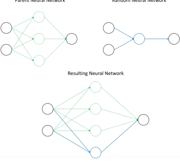
SLM bases its premises on GSGP’s mutation operator, developing a mutation operator that performs a linear combination on two individuals, one from the existing population (𝐼*) and a randomly

generated individual (𝐼9). The mutation will be performed by including 𝐼9 on a branch of 𝐼*. In this

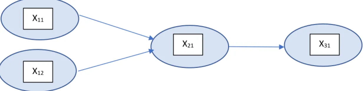
scenario, 𝐼9 will be the simplest form of a multilayered neural network, one with a single hidden layer

containing a single hidden neuron, as shown in Figure 8. This neural network is the one that is going to be merged through mutation to the original ANN.

Figure 8 - Simplest form of a multilayered artificial neural network

A single neuron is added to each hidden layer. Having a number of layers 𝑁 ∈ [3, +∞[, the new neuron added to layer 𝐿:, takes as input layer 𝐿:− 1’s data and gives output to new neurons of the layer

𝐿_:+ 1, or to the output layer for the case of the last hidden layer (Figure 9). The degree of impact of the mutation will be controlled by the mutation step parameter ((Gonçalves, 2016; Gonçalves et al., 2015b). Any activation function can be assigned to the generated neurons, although it should be non-linear to be able learn non-non-linearities from the data. The semantic impact of this mutation is weighted by the connection between the new neuron and the output layer neurons that is the learning step parameter, interchangeable for all connections. The input weights from the layer previous to the added neuron are all randomly generated. There are no restrictions applied to the weights’ initialization.

X12

X11