Elsevier Editorial System(tm) for Applied Soft Computing
Manuscript Draft
Manuscript Number: ASOC-D-18-02084
Title: Classification of mice hepatic granuloma microscopic images based on a deep convolutional neural network
Article Type: VSI: BioMedical Data Analysis
Keywords: Hepatic Granuloma; Microscopic imaging; Image Classification; Deep Learning
Corresponding Author: Dr. Fuqian Shi,
Corresponding Author's Institution: Wenzhou Medical University First Author: Yu Wang, MD
Order of Authors: Yu Wang, MD; Yating Chen, MD; Ningning Yang, MD; Longfei Zheng, MD; Nilanjan Dey, PhD; Amira S Ashour, PhD; V.
July 1, 2018 Editor-in-Chief
Applied Soft Computing Dear Editor,
I am honored to submit our novel and unique contribution manuscript titled: “Classification of mice hepatic granuloma microscopic images based on a deep convolutional neural network”, to your esteemed journal “Applied Soft Computing: VSI: Bio-medical Data Analysis” for kind consideration and publication.
Hepatic granuloma develops in the early stage of liver cirrhosis which can seriously injury liver health. At present, medical microscopic images assessment is necessary for various diseases and employing artificial intelligence technology to assist pathology doctor in pre-diagnosis is the trend of future medical development. In this paper, we try to classify mice liver microscopic images of normal, granuloma-fibrosis1, granuloma-fibrosis2 using convolutional neural networks and 2 conventional machine learning methods: support vector machine and random forest. We also propose a method of data preparation to deal with the problem of insufficient image number and recognizable texture features are extracted and selected using gray level co-occurrence matrix, local binary pattern and pearson correlation coefficient. With the contrast of other classifiers in this paper, we evaluate our own convolutional neural networks in classification accuracy which is 82.78% and confusion matrix, which are satisfied and have clinical significance.
We are very much honored to submit this manuscript to your Journal. We chose the Applied Soft Computing because of its reputation and because we felt this as the most appropriate target for this contribution.
We confirm that the work described has not been published previously (except in the form of an abstract, a published lecture or academic thesis, that it is not under consideration for publication elsewhere, that its publication is approved by all authors and tacitly or explicitly by the responsible authorities where the work was carried out, and that, if accepted, it will not be published elsewhere in the same form, in English or in any other language, including electronically without the written consent of the copyright-holder.
We confirm no conflict of interest. Thank you very much.
Best regards,
Corresponding author#
Fuqian Shi, Ph. D, IEEE Senior Member
#7B-219, Wenzhou Medical University, Wenzhou, 325035, P.R. China Tel. +86-577-86689913
e-mail: [email protected] Cover Letter
Classification of mice hepatic granuloma microscopic images
based on a deep convolutional neural network
Yu Wang1, Yating Chen1, Ningning Yang1, Longfei Zheng1, Nilanjan Dey2, Amira S. Ashour3, V. Rajinikanth4, João Manuel R.S. Tavares5, and Fuqian Shi1, *
1. College of Information and Engineering, Wenzhou Medical University, Wenzhou 325035, People Republic of China
2. Department of Information Technology, Techno India College of Technology, West Bengal, 740000, India
3. Department of Electronics and Electrical Communications Engineering, Faculty of Engineering, Tanta University, Tanta 31111, Egypt
4. Department of Electronics and Instrumentation Engineering., St. Joseph’s College of Engineering, Chennai 600119, Tamilnadu, India
5. Instituto de Ciência e Inovação em Engenharia Mecânica e Engenharia Industrial, Departamento de Engenharia Mecânica, Faculdade de Engenharia, Universidade do Porto, Porto, Portugal
* Corresponding author: Fuqian Shi, email: [email protected], Tel.: +86-577-86689913, Fax: +86-577-86699222
This work is supported by Zhejiang Provincial Natural Science Foundation (Grant no: LY17F030014).
Declarations of interest: none
Abstract
Hepatic granuloma develops in the early stage of liver cirrhosis which can seriously injury liver health. At present, the assessment of medical microscopic images is necessary for various diseases and the exploiting of artificial intelligence technology to assist pathology doctors in pre-diagnosis is the trend of future medical development. In this article, we try to classify mice liver microscopic images of normal, granuloma-fibrosis1 and granuloma-fibrosis2, using convolutional neural networks and two conventional machine learning methods: support vector machine and random forest. We also propose a method of data preprocessing to deal with the problem of insufficient image number and recognizable texture features are extracted and selected using gray the level co-occurrence matrix, local binary pattern and pearson correlation coefficient. Relatively to the other classifiers studied, the suggested solution based on convolutional neural networks was evaluated in terms of classification accuracy, which was of 82.78%, and confusion matrix, which shown to be promising and with clinical significance, and revealed its preeminence.
Keywords: Hepatic Granuloma; Microscopic imaging; Image Classification; Deep Learning
1 Introduction
Hepatic cirrhosis is a degenerative and chronic liver disease, which has as the main characteristic the fact that normal liver cells been replaced by collagenous scar (fibrosis). In the early stage of cirrhosis, especially in primary biliary cirrhosis, the pathologist may uncover one or more granulomas in a biopsy specimen, diagnosing the stage of underlying liver injury [1]. Granuloma is commonly defined as a distinct nodular lesion formed by macrophages and their evolution of
*Manuscript
localized infiltration and proliferation, which are presented as red-brown and annular grouped cells arranging disorderly and densely. All these characteristics are commonly delineated in microscopic images.
Microscopic imaging is as an important medical imaging modality, which carries rich but complex information including about the various structures of biological tissue, the state of different cells and others that pathology doctors demand. However, the complexity of the acquired images and doctors’ subjectivity often cause disagreement even among experienced pathologists [2], which suggests an increasing demand for robust and stable computational approaches to improve the diagnosis efficiency [3, 4, 5].
In recent years, deep learning, especially convolutional neural networks (CNNs) [6], as an excellent machine learning method for image classification, has also been proposed to analyze images in digital pathology. There have been many researches in digital microscopic image analysis employing CNNs. Philipp kainz et al. [7] used CNN classifier architectures to segment and classify the colorectal cancer in histopathological images, suggesting a new combination of separate-net and object-net. In [8], epithelial and stromal regions in stained H&E images were automatically extracted features and classified using deep CNNs, which outperformed the traditional classification methods. Although several approaches based on CNNs have already proposed with success, the comparations among them are not available. In [9], a comprehensive tutorial with seven use cases, such as nuclei segmentation, lymphocyte detection and mitosis detection, has been presented, outlining a guide for other researchers to study in digital pathology domain by leveraging CNNs.
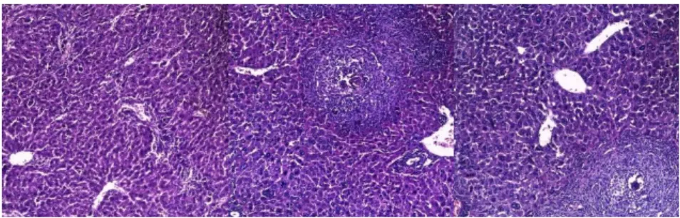
A typical microscopic image of hepatic granuloma encompasses four tissue components: multinuclear giant cells derived from macrophage, cytoplasm, epithelia and lymphocytes. The multinuclear giant cells are grouped by epithelia that connect other tissues appearing fibrous, generating the granuloma annular, in which the numerous nucleuses usually arrange densely, and centre lymphocytes. The difference between normal and abnormal microscopic images can be shown in Figure 1. In the figure of granuloma-fibrosis2, the annular area of granuloma is larger and the background is more fibrotic.
Figure 1 – Form the left to the right: mice microscopic images of normal and two degrees of hepatic granuloma.
In this article, we describe our CNN-based multi-classification strategy for the mice hepatic granuloma microscopic images taken into account three classes: normal, granuloma-fibrosis1 and granuloma-fibrosis2. To our knowledge, there are no previous studies on hepatic granuloma
microscopic images based on the application of artificial intelligence technology. Thus, referring to works on other disease microscopy images, we also propose a method of data preprocessing to overcome the problem of insufficient image numbers. In order to evaluate the performance of the proposed CNN model, we compare the classification results against the results obtained by other two traditional classifiers: support vector machine with polynomial kernel (SVM) [10] and random forest (RF) [11], as well as against a famous and classic CNN model: AlexNet [12]. All the training processes were based on 4-fold cross validation for assuring the robustness of the final results. In addition, when employing conventional machine learning approaches, we use gray level co-occurrence matrix (GLCM) and local binary pattern (LBP) to extract texture features including energy, contrast, correlation and uniformity. Various features could be calculated through GLCM, the eight features used in this work are the widespread and most typical features in the field of image feature extraction. Furthermore, hepatic granuloma and local annular fibrosis can be well described by LBP. Therefore, we hypothesized that this two feature extraction methods can attain the information about image textural characteristics. After attaining all the features of the input images, we use pearson correlation coefficient as the feature selection method to remove useless features from complete feature set, which also benefits to the final classification performance. In terms of accuracy and details in confusion matrix, our proposed CNN performed better: the total accuracy was 82.78% (Normal class, 92.5%; Granuloma-fibrosis1, 76.67%; Granuloma-fibrosis2: 79.17%). Three postgraduates of the pathology department exchanged advices of what features should be extracted and how to split the datasets with us, making our experiment with more clinical practice significance.
The majority of previous works regarding hepatic cirrhosis image analysis is mainly focused on ultrasound images, which usually include tasks of image segmentation and classification. In [13], a computer-aided cirrhosis diagnosis system based on ultrasound images was proposed, and a CNN was employed to extract deep level features which were proved better than hand-crafted features like HOG and LBP. Suganya and Rajaram achieved accurate categorization of cirrhosis ultrasound images using the methods: modified Laplacian pyramid nonlinear diffusion filter as image preprocessing and gray level co-occurrence matrix, local binary pattern and scale invariant feature transform as image feature extraction. In the result of image classification using a CNN, the accuracy was of 100% that overcame considerably the accuracies obtained by decision tree and SVM [14]. When confronting onerous hand-crafted features, feature selection is an ideal solution for researchers to improve the classification performance. Some classic and efficient approaches gave been suggested, such as genetic algorithm [15], particle swarm optimization [16] and singular value decomposition [17]. In [18], liver cirrhosis, normal liver and hepatocellular carcinoma were classified through applying the multiresolution wavelet packet texture descriptors. With the feature selection method of Genetic algorithm-SVM, the classification performance did improve significantly.
Although numerous differences exist between ultrasound images and microscopic images about liver cirrhosis, we can still refer them to improve our solution. On one hand, the original ultrasound images of liver cirrhosis should not be cropped neither other data augmentation methods used, otherwise that would be unavailable for physicians to diagnose liver disease. However, when applying CNNs in tasks of image classification, a large amount number of data is
indispensable to avoid overfitting. But as to medical image data, it is always difficult to obtain sufficient and qualified image data. Obviously, data augmentation has widely used in various kinds of medical image applications [6], such as to skin cancer [19], lung cancer [20] and cell detection [21]. Our new method of data preprocessing towards hepatic granuloma microscopy focuses on how to crop the input image in order to obtain an ideal classification result by the CNN model. On another hand, liver cirrhosis in the ultrasound imaging shows the liver capsule as thickness with jagged, wavy and stepped changes. Comparatively, microscopic images can carry more rich information even after cropped, providing the accurate degree of fibrosis and the numbers of granuloma annular.
The rest of this article is structured as followings: The details of the main used methods are provided in Section 2. Then, the specific explanations of our experimental setups are given in Section 3. The results and discussion are presented in Section 4. Concluding remarks and future works are pointed out in Section 5.
2. Methods
2.1 Convolutional neural networks
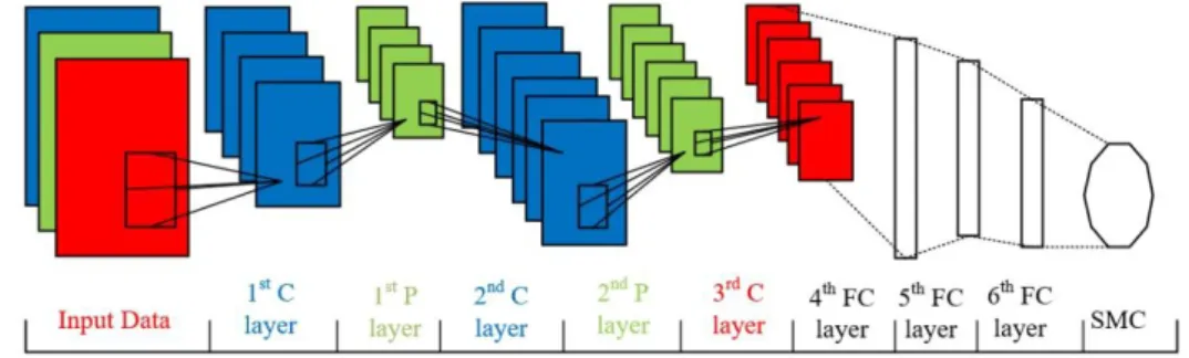
Convolutional neural networks are from the artificial neural network field with a strong deep learning ability. Deep learning algorithms are based on the deep architectures of continuing layers which orderly separate into convolutional layer, full-connection layer and the output layer. In our CNN architecture, the output layer is the Softmax classifier (SMC) [22], which is a common choice for multi-classification tasks. And, after been cropped, the microscopic images are fed into every single layer successively. The framework of our proposed CNN architecture is shown in Figure 2.
Figure 2 Proposed CNN architecture.
2.1.1 The architecture of the convolutional layers
Typically, the convolutional layers include some alternative convolutional layers (C layers) and max-pooling layers (P layers). The convolution and max-pooling feature maps can be built by these C and P layers, respectively. Then, strong features can be extracted from the feature maps and then combined.
Let’s assume that X (m,n)k
represents the inputting 2-dimensional map of the k-th channel, and
l (m,n)
k
H is the convolution kernel, being m and n the dimensionality and k and l the number of input channels and output channels so the size of the convolution kernel be k l . Hence, we have:
-1 -1 -1 0 0 0 ( , ) ( , ) * ( , ) ( , ) ( , ){ 0,1,..., ; 0,1,..., ; 0,1,... } l k kl K I J k kl k i j Y m n X m n H m n X m i n j H i j k K i I j J
(1) Where l (m,n)Y is the outputting 2-dimensional feature map of the l-th channel and kl H (m,n), with size of I J , means the 2-dimensional kernel of the l-th column and k-th row.
After attained the l (m,n)
Y , the result must be multiplied by the activation function: Rectified Linear Unit (ReLU) [29] before transferring the data downward to the next layer; the used activation function is:
(x)
max(0, x)
(2)The range of ReLU function is
[0,
)
.2) P layers
The features obtained by the convolution layers can be processed again in the other layers, thus CNN setups pooling layers to reducing the calculated quantity. In this work, we employ the max-pooling method which attains to compute the maximum value of a given feature in a certain feature map.
2.1.2 The architecture of full-connection layers
In full-connection layers (FC layers), every node is connected to other nodes from the adjacent layers. Calculated by matrix multiplication with vectors, full-connection layers transform each input feature into a vector.
2.1.3 Pipeline of the proposed CNN based classifier
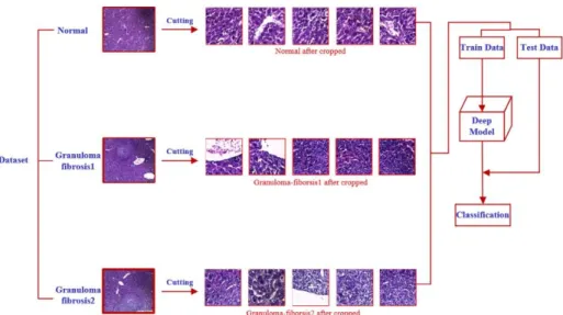
Figure 3 presents the whole process of liver classification into normal, hepatic granuloma-fibrosis1 and hepatic granuloma-fibrosis2 tissues in microscopic images. Firstly, the raw microscopic images are labelled, cropped and separated before fed into the proposed CNN model. This step is described in Section 3. Secondly, we train the CNN model through train data that are split into four sets to conduct 4-fold cross validation. And finally, we use test data to evaluate the completed CNN model and assess the classification accuracy.
Figure 3 The pipeline of the proposed CNN based classification.
2.2 Pipeline of the SVM and RF based classifiers
The developed pipeline of the SVM and RF based classifiers, shown in Figure 4, can be resumed by the following five steps:
Step 1: Labelling of all the raw microscopic images and cropped them to the size of
256 256
pixels;Step 2: Extraction of the texture features using the GLCM and LBP methods; Step 3: Division of the input image dataset into training and testing datasets; Step 4: Training of the SVM and RF based classifiers using the training data; Step 5: Evaluation the classification performance of the classifiers.
Figure 4 Pipeline of the SVM and RF based classifiers.
2.2.1 Gray level co-occurrence matrix
digital images through calculating the spatial relationship of each image pixel. The implemented method is based on the joint conditional probability density among image grayscale levels, whose function is: L-1 L-1 0 0 ( , | , ) (( , ) | ( , ) , ( , ) ; x, y 0,1, 2,..., N 1) i j Q i j d x y f x y i f x dx y dy j
(3)where
(i,j)
is a pair of image pixels with distance equal to d and an angle θ equal to: 0 , 45 , 90 or135 , and L is the maximal gray level value presented in the input image of size N*N . Therefore,Q i j d
( , | , )
can be also defined taken into account the emergence probability of the given pair pixels, which arei=f(x,y)&j=f(x+dx,y+dy)
, where(x,y)
represents the pixel location in the input image, with the distance d and angleθ, respectively. Various image features can be extracted from GLCM. Referring the current research methods of analyzing microscopic images and combining with the characteristics of granuloma microscopy, we choose eight texture features: energy, contrast, entropy, correlation, mean, texture variance, dissimilarity and homogeneity: 1) Energy: -1 1 2 0 0ner
=
( , )
L L i jE
gy
Q i j
(4) 2) Contrast: -1 -1 * 2 * 0 0( , ) | - | (
( , )
( , ))
L L t i jC
Q i j i j
Q i j
normalize Q i j
(5) 3) Entropy: -1 1 0 0-
( , ) ln(
( , ))
L L i jE
Q i j
Q i j
(6) 4) Correlation: -1 -1 1 2 0 0 1 2(
)(
)
( , )
L L i ji
j
Q i j
C
(7) where: -1 -1 1 0 0( , )
L L i jiQ i j
(8) -1 -1 2 0 0( , )
L L i jjQ i j
(9) -1 -1 2 1 1 0 0(
)
( , )
L L i ji
Q i j
(10) -1 -1 2 2 2 0 0(
)
( , )
L L i jj
Q i j
(11) 5) Mean:-1 1 0 0
Mean=
( , )
L L i jQ i j
i
(12) 6) Texture Variance -1 1 2 0 0=
( , ) (
)
L L i jTV
Q i j
i
Mean
(13) 7) Dissimilarity: -1 1 0 0D=
( , ) |
|
L L i jQ i j
i
j
(14) 8) Homogeneity: -1 1 2 0 01
H=
( , )
1 ( - )
L L i jQ i j
i j
(15)2.2.2 Local binary pattern
Local binary pattern (LBP) method [24] intends to describe the local features of an input image and has been improved according to several novel variants, such as circular the LBP method [25] used in this work. The original LBP algorithm divides the image into many 3 3 cells, where the gray value of a central pixel determines the neighborhood threshold. In each cell, all the gray values of other eight pixels neighboring the central pixel are compared against a threshold value; if the value of the surrounding pixel is greater than of the central pixel, then the pixel is marked as 1 (one) or 0 (zero).
A formal description of the LBP operator is:
-1 0
( ,
)
2
(
- )
P P c c P c PLBP x y
s i
i
(16)where
(x ,y )
c c is the coordinates of the central pixel with gray value denoted byi
c, andi
Pmeans the gray values of the surrounding P pixels, and s is a sign function defined as:
1 0 ( ) 0 if x s x esle (17)
By computing these two functions, the LBP value can be obtained, which is a two-valued binary code. The LBP feature values are represented here by a vector consisted of ten characteristics.
2.2.2 Feature selection
Texture feature selection is an efficient method to reduce characteristic dimension in medical microscopic image classification. With a proper feature selection technique, we can not only shorten the execution time in the training process, but also improve the classifier performance. Pearson correlation coefficient (PCC) [26] is a suitable approach to measure the correlation between feature variables, as well as to assist researchers to understand the relationship between characteristics and response variables. The results of PCC are ranged between 1 (one) to -1 (minus one), which can give the strength and monotonicity of the variables’ relationship.
3. Experimental setup
3.1 Used dataset and preprocessing
The used hepatic cirrhosis microscopic images were labelled as normal, granuloma-fibrosis1 and granuloma-fibrosis2 without lesions location label. Our labelled dataset contains 30 mice liver histopathological images of size
1536 2048
pixels divided into 10 normal images, 10 granuloma-fibrosis1 images and 10 granuloma-fibrosis2 images.Firstly, all the original images were cropped in patches of size equal to
256 256
pixels, and then after disordered, the patches were recombined to new images also of size equal to1536 2048
pixels; secondly, we repeated the first step to obtain the final patches and separated them into three datasets: training dataset, validation dataset and testing dataset. Except for the CNN model, the validation and the training datasets were mixed.Figure 5 An original input microscopic image (left) and the correspondent image after rearrange and combine the built image patches (right)
With this data preprocessing, we enlarged the image dataset from 30 to 1,440 images (expand 48 times) and were divided into 3 image data sets: one of 720 training images, another one with 360 validation images and a last one of 360 testing images. That is, we augmented our initial dataset of 30 medical microscopic images to a dataset of 1,440 images. The details of the achieved dataset are given in Table.1.
Table.1 The dataset of the microscopic images after augmentation Microscopic image types Training images Validation images Testing
images Total images
Normal 360 120 120 480 (10*6*8=480)
Granuloma-fibrosis1 360 120 120 480 (10*6*8=480)
Granuloma-fibrosis2 360 120 120 480 (10*6*8=480)
(2)
(3)
Figure 6 Examples of five cropped images resultant from normal (1), granuloma-fibrosis1 (2) and granuloma-fibrosis2 (3) images
3.2 Extracting and selecting features from patches
We extracted the texture features from all patches by using GLCM and LBP methods, obtaining 18 characteristics to train our CMN based classifier. Then, we selected the optimal features using the PCC based approach.
3.3 Training model with SVM and RF
SVM and RF based classifiers were trained with 1,440 cropped images of size equal to
256 256
pixels. For the SVM classifier, we used LIBSVM [27]. All the images were separated using 4-fold cross validation before every experiment, and we employed the polynomial kernel and 5-fold cross-validation to seek the optimal parameters of the polynomial kernel according to a stride of optimization of 0.1 and raging from -5 to 5. For the RF classifier, a quarter of 1,440 image data was randomly selected as testing data for cross validation; we adopted 180 estimators, i.e. the number of decision trees used, and a random generator number of 20.3.4 Details of CNN layer
The proposed CNN architecture, which was motivated by the AlexNet architecture, consists of 3 convolutional layers, 3 pooling layers, 3 full-connection layers and the output layer with SMC. Table 2 presents details of each layer (Figure 2). The size of the input data is equal to
224 224
after normalization, and R, G, B are the 3 input color channels. For C1~C3, the output feature maps of every layer are of size equal to:C
1=55 55
,P
2=27 27
,C
2=12 12
,P
2=6 6
and
C
3=6 6
, respectively. Correspondingly, the outputted of every layer has the size of: 64, 64, 32, 32, and 16. A function that describes the relationship among the other parameters of layers is:Size(InputData)
(Kernel)
2 Pad
Size(Feature map)=
Size
1
Stride
(18) For example, the size of feature map in P1 layer is
55 55
, calculated as:224 8 2 0
Size(C1 Feature map)=
1=55
4
Table 2 Output and parameters of the used CNN model.
layers ratio Input Data (3, 224, 224) C 1 (64, 55, 55) 8 4 0 P 1 (64, 27, 27) 3 2 0 C 2 (32, 12, 12) 8 2 2 P 2 (32, 6, 6) 3 2 0 C 3 (16, 6, 6) 3 1 1 FC 1 (1024) 0.5 FC 2 (512) 0.5 FC 3 (3)
3.5 Parameter setting for training the CNN
In the process of training the proposed CNN model, the learning rate policy determines how to adjust the learning speed of each layer, and the adopted parameters were: a base learning rate (base-lr) of 0.01; the learning method (lr-policy) was “step”; and “gamma” and “stepsize” were 0.5 and 10000, respectively. Another critical parameter setup is the approach of seeking optimal solution, which is “AdaDelta” in this work [28].
3.6 Experimental platform
All experiments were conducted on a NVIDIA GeForce GTX 1070 GPU under the Community Enterprise Operating System (CentOS) 7.3 and on a PC (Intel Core (TM) i7-6700HQ, 2.6 GHz processor with 8 GB of RAM). The software implementation was performed using MATLAB 2016A and Caffe framework [29].
4 Results and Discuss
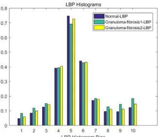
The image features extracted using GLCM method are indicated in Table 3, which includes the mean values of all 8 texture features calculated from the 1,440 microscopic patches built after taking into account the angles of: 0 , 45 , 90 , and135 . Figure 7 presents the differences found among the three types of microscopy images in terms of the LBP characteristic vector.
Table 3 Mean values of the 8 texture features extracted using the GLCM method
Texture feature Normal Granuloma-Fibrosis1 Granuloma-Fibrosis2
Contrast 0.1149 0.1018 0.0945 Correlation 0.5011 0.6711 0.6270 Energy 0.8951 0.8835 0.8939 Homogeneity 0.3942 0.4727 0.4596 Entropy 2.6811 2.8128 2.8562 Dissimilarity 0.8189 0.7919 0.7947 Texture Mean 4.1104 3.7889 3.9598 Variance 2.4657 2.9229 3.0670
Figure 7 The histogram of the LBP feature values for the three image types under study
Table 4 The Pearson Correlation Coefficient results Texture feature PCC (scores,
p-value)
Texture feature PCC (scores, p-value) Contrast (0.318, 8.652e-13) LBP feature-vetor1 (0.190, 2.747e-05) Correlation (0.438, 6.397e-24) LBP feature -vetor2 (0.196, 1.499e-05) Energy (0.098, 0.031) LBP feature -vetor3 (0.240, 9.687e-08) Homogeneity (0.453, 9.650e-26) LBP feature -vetor4 (0.365, 1.346e-16) Entropy (0.396, 1.586e-19) LBP feature -vetor5 (-0.050, 0.270) Dissimilarity (0.443, 1.331e-24) LBP feature -vetor6 (0.188, 3.221e-05) Texture Mean (0.020, 0.646) LBP feature -vetor7 (0.131, 0.003)
Variance (0.205, 5.908e-06) LBP feature -vetor8 (0.167, 0.000) LBP feature -vetor9 (-0.008, 0.858) LBP feature -vetor10 (0.157, 0.000)
After the feature selection step, we are aware of the features that are useful or useless. We can find that in Table 4, the high positive correlations and high scores are noted such as for Correlation, Homogeneity, Contrast and Dissimilarity; on other hand, the LBP feature-vector5 and vector9 are negative, meaning that these features may be weak. These experimental results are consistent with the actual diagnosis of liver cirrhosis: as in the initial stage, the histopathological images of hepatic granuloma ought to have higher Correlation and lower Contrast because liver granulomas will group cells disorderly and densely arranged. Actually, in our experiment, the texture features extracted using the GLCM method are stronger than the LBP based features.
The confusion matrix [30] is a visualization tool to assess the performance of a classifier commonly used in artificial intelligence technology. In image multi-classification tasks, the confusion matrix displays each class result and compares the classification results with the actual measured values.
Table 5 presents the classification results of every class elaborately in a confusion matrix. 100 images were correctly predicted in 120 images labelled “Normal”; there were 36 “Normal” images predicted to be “Granuloma-fibrosis1”; and 52 images were misjudged to “Granuloma-fibrosis2” instead of “Normal”. Table 6 indicates the accuracy computed for each class under study.
Table.5 The confusion matrix of the classification results using SVM-Polynomial Normal Granuloma-fibrosis1 Granuloma-fibrosis2
Normal 100 5 15
Granuloma-fibrosis1 7 101 12
Granuloma-fibrosis2 10 9 101
Table.6 The accuracy of the classification results using SVM- Polynomial
Microscopic image types Accuracy Total / True
Normal 83.33 % 120 / 100
Granuloma-fibrosis1 84.17 % 120 / 101
Granuloma-fibrosis2 84.17 % 120 / 101
The correspond results as RF, AlexNet and proposed CNN based classifiers are presented in Tables 7 to 12. Compared with the SVM, RF and AlexNet based classifiers, according to the confusion matrix, our proposed CNN based model has many advantages: Firstly, the Normal class gains the highest accuracy score: 92.5%, and for the cases of misjudgment: only 7 Normal samples were wrongly classified to Granuloma-fribrosis1, which can be justified by the fact that the early stage of liver cirrhosis resembles the normal state. Secondly, for the Granuloma-fibrosis 1 and 2, although the accuracy is inferior than the ones of SVM and RF based classifiers, the number of Granuloma-fibrosis2 misjudged to Normal is too high, which could nonplus the pathologists due to the evident differences between them. However, the proposed CNN and AlexNet based classifiers avoid this case, which also suggests that the CNN based classifier is superior to the traditional classifiers studied in this work for comparison purpose. In addition, our CNN based classifier overcome the AlexNet classifier by having a more concise architecture: 3 C and 3 P layers, 3 FC layers and the SMC classifier.
Table 7 Confusion matrix of the classification results obtained using the RF based classifier Normal Granuloma-fibrosis1 Granuloma-fibrosis2
Normal 92 8 20
Granuloma-fibrosis1 9 96 15
Granuloma-fibrosis2 18 9 93
Table 8 Accuracy of the classification results obtained using the RF based classifier
Microscopic image types Accuracy Total / True
Normal 76.67 % 120 / 92
Granuloma-fibrosis1 80 % 120 / 96
Granuloma-fibrosis2 77.5 % 120 / 93
Table 9 Confusion matrix of the classification results obtained using the AlexNet classifier Normal Granuloma-fibrosis1 Granuloma-fibrosis2
Normal 108 10 2
Granuloma-fibrosis1 12 86 22
Granuloma-fibrosis2 7 15 98
Table 10 Accuracy of the classification results obtained using the AlexNet classifier
Microscopic image types Accuracy Total / True
Normal 90 % 120 / 108
Granuloma-fibrosis1 71.67 % 120 / 86
Table 11 Confusion matrix of the classification results obtained using the proposed CNN based classifier
Normal Granuloma-fibrosis1 Granuloma-fibrosis2
Normal 111 7 2
Granuloma-fibrosis1 6 92 22
Granuloma-fibrosis2 5 20 95
Table 12 Accuracy of the classification results using the proposed CNN based classffier
Microscopic image types Accuracy Total / True
Normal 92.5 % 120 / 111
Granuloma-fibrosis1 76.67 % 120 / 92
Granuloma-fibrosis2 79.17 % 120 / 95
Table 13 presents the global accuracy obtained by each of the four classifiers under comparison. Despite our experimental results are not satisfactory as to the RF based classifier, we cannot deem that the RF classifier is unpromising as the lack of enough training data can also lead to failure. In [13, 14, 18], very high classification accuracies and of other evaluation criteria do notarize the success of this classifier. However, when in multi-classification tasks, it is not enough only to attain a high classification accuracy. We also completed the 2-classification task in the mice hepatic microscopic images which reached a satisfied classification accuracy in our previous works [31].
Table 13 Global accuracy obtained by each classifier
5 Concluding Remarks and Future works
This research article has presented our designed CNN architecture that shown to be competent to classify mice liver microscopic images into normal, granuloma-fibrosis1 and granuloma-fibrosis2 cases. In order to assess the performance of the proposed CNN based classifier, we conducted the classification experiment using other three common classifiers: SVM with polynomial kernel, RF and AlexNet. The experimental results were discussed evaluated based on the confusion matrixes built. Moreover, the results of the SVM and RF based classifiers were also satisfactory, suggesting that our methods of data preprocessing and feature extraction are reasonable. After the feature selection step, we figured out that the texture features obtained using the GLCM method are highly distinguishable.
In future works, we still entail to deal with the problem of insufficient number of training images. Because when we trained the classifiers by augmenting data to avoid overfitting, the classification results were not quite desirable which should be better if we can acquire sufficient images. And in
Classifiers Accuracy
RF 78.05 %
SVM-Polynomial 84.17 %
AlexNet 81.11 %
order to assist pathologists more comprehensively, apart from the final classification results, we should also try to segment the lesion areas: the annular granulomas and other diagnostic relevant information employing CNNs.
Acknowledgement
Dalia S. Ashour, Assistant Professor of Medical Parasitology and Dina M. Aboraya, Lecturer of Medical Parasitology, Medical Parasitology Department, Faculty of Medicine, Tanta University, in Egypt, performed the microscopic experiment and preprocessed the acquire image dataset.
Reference
[1] Wehmeyer, M., et al, Clinical presentation, natural history and treatment of hepatic sarcoidosis: A case-series of 39 patients with histologically proven hepatic sarcoidosis, Journal of Hepatology. 68 (2018) S616-S617.
[2] Pavlides M, Birks J, Fryer E, et al, Interobserver Variability in Histologic Evaluation of Liver Fibrosis Using Categorical and Quantitative Scores, American Journal of Clinical Pathology. 147 (4) (2017) 364.
[3] Shouvik Chakraborty, Sankhadeep Chatterjee, Nilanjan Dey, Amira S. Ashour, Ahmed S. Ashour, Fuqian Shi, Modified cuckoo search algorithm in microscopic image segmentation of hippocampus, Microscopy Research and Technology, Microscopy Research and Technique. 80 (10) (2017) 1051-1072.
[4] Zairan Li, Nilanjan Dey, Amira S. Ashour, Convolutional neural network based clustering and manifold learning method for diabetic plantar pressure imaging dataset, Journal of Medical Imaging and Health Informatics. 7 (3) (2017) 639-652.
[5] Amira S. Ashour, Samsad Beagum, Nilanjan Dey, Ahmed S. Ashour, Dimitra Sifaki Pistolla, Gia Nhu Nguyen, Dac-Nhuong Le, Fuqian Shi, Light microscopy image de-noising using optimized LPA-ICI filter, Neural Computing and Applications. 29 (12) (2018) 1517-1533.
[6] Rawat W, Wang Z, Deep Convolutional Neural Networks for Image Classification: A Comprehensive Review, Neural Computation. 29(9) (2017) 1.
[7] Kainz, P., M. Pfeiffer, and M. Urschler, Segmentation and classification of colon glands with deep convolutional neural networks and total variation regularization, PeerJ. 5 (3) (2017) e3874. [8] Xu, J., et al., A Deep Convolutional Neural Network for segmenting and classifying epithelial and stromal regions in histopathological images, Neurocomputing. 191 (2016) 214-223.
[9] Andrew, Janowczyk, M. Anant, Deep learning for digital pathology image analysis: A comprehensive tutorial with selected use cases, Journal of Pathology Informatics. 7 (1) (2016) 29. [10] Majdar R S, Ghassemian H, A probabilistic SVM approach for hyperspectral image classification using spectral and texture features, International Journal of Remote Sensing. 38 (15) (2017) 4265-4284.
[11] Jog A, Carass A, Roy S, et al., Random forest regression for magnetic resonance image synthesis, Medical Image Analysis. 35 (2017) 475-488.
[12] Alex Krizhevsky, Ilya Sutskever, Geoffrey E. Hinton, ImageNet Classification with Deep Convolutional Neural Networks, in Proc. NIPS, Advances in Neural Information Processing Systems 25 (NIPS 2012). 2012.
Ultrasound Image Classification, Sensors. 17 (1) (2017) 149.
[14] Suganya R, Rajaram S, An efficient categorization of liver cirrhosis using convolution neural networks for health informatics, Cluster Computing. 3 (2017) 1-10.
[15] Jiang S, Chin K S, Wang L, et al., Modified genetic algorithm-based feature selection combined with pre-trained deep neural network for demand forecasting in outpatient department, Expert Systems with Applications. 82 (C) (2017) 216-230.
[16] Xue B, Zhang M, Browne W N, Particle swarm optimization for feature selection in classification: a multi-objective approach, IEEE Trans Cybern. 43 (6) (2013) 1656-1671.
[17] Meuwissen T, Indahl U G, Ødegård J, Variable selection models for genomic selection using whole-genome sequence data and singular value decomposition, Genetics Selection Evolution, 49 (1) (2017) 94.
[18] Virmani J, Kumar V, Kalra N, et al., SVM-based characterization of liver ultrasound images using wavelet packet texture descriptors, Journal of Digital Imaging. 26 (3) (2013) 530-543. [19] Andre Esteva, Brett Kuprel, Roberto A. Novoa, Justin Ko, Susan M. Swetter, Helen M. Blau & Sebastian Thrun, Dermatologist -level Classification of Skin Cancer with Deep Neural Networks, LETTER. 2017.
[20] Yu K H, Zhang C, Berry G J, et al., Predicting non-small cell lung cancer prognosis by fully automated microscopic pathology image features, Nature Communications. 7 (2016) 12474. [21] Pan X, Yang D, Li L, et al., Cell detection in pathology and microscopy images with multi-scale fully convolutional neural networks, World Wide Web-internet & Web Information Systems. 11 (2018) 1-23.
[22] Duan K, Keerthi S S, Chu W, et al., Multi-category Classification by Soft-Max Combination of Binary Classifiers, Multiple Classifier Systems, International Workshop, Mcs 2003, Guilford, Uk, June 11-13, 2003, Proceedings. DBLP. (2013) 125-134.
[23] Kobayashi T, Sundaram D, Nakata K, et al, Gray-level co-occurrence matrix analysis of several cell types in mouse brain using resolution-enhanced photothermal microscopy, Journal of Biomedical Optics. 22 (3) (2017) 36011.
[24] Wan S, Lee H C, Huang X, et al., Integrated local binary pattern texture features for classification of breast tissue imaged by optical coherence microscopy, Medical Image Analysis. 38 (2017) 104-116.
[25] Ojala, T., M. Pietikainen, and T. Maenpaa, Multiresolution Gray Scale and Rotation Invariant Texture Classification with Local Binary Patterns, IEEE Transactions on Pattern Analysis and Machine Intelligence. 24 (7) (2002) 971-987.
[26] Reggiani E, D’Arnese E, Purgato A, et al., Pearson Correlation Coefficient Acceleration for Modeling and Mapping of Neural Interconnections, Parallel and Distributed Processing Symposium Workshops, IEEE. (2017) 223-228.
[27] Fan, R., Chen, P., Lin, C., et al., Working Set Selection Using Second Order Information for Training Support Vector Machines, Journal of Machine Learning Research. 6 (4) (2015) 1889-1918.
[28] BAIR, Deep learning framework, online: http://caffe.berkeleyvision.org/tutorial/solver.html [29] Jia, Yangqing, Shelhamer, et al., Caffe: Convolutional Architecture for Fast Feature Embedding, (2014) 675-678.
[30] Ding J, Hu X H, Gudivada V, A Machine Learning Based Framework for Verification and Validation of Massive Scale Image Data, IEEE Transactions on Big Data. 1 (1) (2017) 99.
[31] Yu Wang, Luying Cao, Nilanjan Dey, Amira S. Ashour and Fuqian Shi, Mice Liver Cirrhosis Microscopic Image Analysis Using Gray Level Co-Occurrence Matrix and Support Vector Machines, Frontiers in Artificial Intelligence and Applications, 296, pp.509-515, in Proc. ITITS 2017, Xian, China