A MODEL FOR THE YIELD CURVE
J. C. Rodrigues da Costa March 20001
Abstract
The starting point is an interrogation about the non-broken character of the term structure of interest rates. Some arguments for that smooth character are presented here, all of which are based upon the assumption that market participants - arbitrageurs and speculators - always try to explore any misalignments discovered in the interest market. This led to the basic concept behind the model that the current short-term rate determines most of the value of the rate level for the subsequent period. A linear model describing that simple relationship is assumed and that constitutes the building block from where one can develop the mathematical equations necessary to work with different sets of market data.
A number of different yield curves were modelled by adjustment to real market data using this basic model, all of them showing a very high quality of the fits when measured by
the non-linear ratio R2. Nevertheless this fact still needs to be confirmed as the examples
were drawn from non-independent markets and from a very short time window.
The model can be improved by simple addition of a liquidity premium depend only upon the maturity of the rates. However, that improvement sophisticates tremendously the mathematical tractability of any real situation without any assurance that this added cost compensates for the increased quality of the fit.
The model is designed around only 3 parameters that can all be interpreted in economic terms. Two of them, in particular, bring a significant improvement over the traditional views frequently extracted from the shape of the yield curve.
Provided future tests confirm the high quality of the basic and the improved (with a liquidity premium) models, both are supportive of the expectation hypothesis (EH) and the liquidity premium hypothesis (LPH).
1
I have to thank to Luís Catela Nunes for his valuable comments about an earlier version of this paper. Of course, any remaining errors are my own fault.
1. Introduction
The shape of the yield curve has intrigued economists for a long time and that trig-gered the search for a series of theories that tried to explain that particular shape. The initial attempts tried to engender a coherent view from the behaviour of the users of money -borrowers and lenders - that could justify the differences between short term and long term interest rates. When those users, by any sort of reasons, demanded more long deposits or loans than short term ones the curve should be upward sloping, and the opposite should occur when their demand for shorter operations was higher than for long ones.
That is, initially it was the general shape of the curve that was the object of the ana-lysis, and from there, basically four schools of thought were produced - the traditional term structure theories: the Expectations Hypothesis (EH), the Liquidity Preference Hypothesis, the Market Segmentation Hypothesis and the Preferred Habitat Theory.
More recently, the search for models to price debt derivatives led to the development of a different series of approaches, all of them based on stochastic calculus. Instead of ex-plaining the overall shape of the curve, these new theories focus on the dynamics of the curve itself, that is, how it might evolve along the time. More specifically, they produce estimates for the interest rate volatility of each maturity so that a price can be attached to that uncertainty. Here less attention is dedicated to the views of the “consumers” of money as these models tend to accept as a starting point some Brownian diffusion process for one or two interest rates without any consideration of the psychological behaviour behind such differential equations.
Beyond the explanations of the qualitative shape of the curve and the models that price the volatility of interest rates, the search here is for a quantitative mathematical model describing that shape in order to help practitioners extract objective financial information from the actual instruments traded in the market.
In fact, if one can define one explicit and (if possible) simple mathematical formula
RT = f(maturity T) with a certain number of parameters, it will be much simpler to fit such
function to the numerical data provided by money and capital markets instruments than the common methods of segmenting the curve into a number of splines or approaching it by so-me form of polynomial or a sum of exponentials. One can also discount the cash-flows pro-duced by a set of different issues of traded T-Bonds using the rates estimated by that formu-la and adjusting the parameters of the model in order to minimise the mean squared error between those market prices and the prices produced by the formula.
The existence of a single formula relating interest rates to maturities also simplifies the estimation of the interest rate for any maturity between two adjacent dates for which that information is available. There is no need to interpolate between those adjacent rates, and so, for a new debt instrument with cash flows between traditional dates, it becomes much simpler to find the appropriate discount factors that are compatible with the current term structure.
The model developed also brings the advantage that the parameters of the formula have an economic meaning which helps in interpreting the “consumers” expectations about future developments in the relevant interest rate market.
2. Literature
One of the most resilient ideas in this field of the yield curve is the concept that in-vestors´ views for the future are always imbedded in the current rates for long-term loans or deposits. When Irving Fisher added the expected inflation rate to the real cost of money to obtain the current nominal interest rates, he implicitly accepted the idea that inflation expectations for the future were a determinant of today´s long-term rates. Long rates must compensate for the expected future inflation and still leave some margin to pay some real return to the investor or to inflict a real cost to the borrower.
It is true that there is a theory that negates any role to the current expectations in the market, the so called Market Segmentation Hypothesis, due to Culbertson. For him, the mar-ket is segmented along the maturity axis because the interest rate for maturity T is simply the outcome of a local equilibrium that is struck between suppliers of funds and borrowers of capital, both of whom can only invest and raise money within a very narrow range of maturities. None of them can consider the demand and the offer of capital in any other segment, even if adjacent to their natural one. This is the result of their risk aversion to the uncertainty of future interest rates and the correspondent volatility of asset prices. So, they always try to match as much as possible the maturities of their assets to the maturities of their liabilities. But that is a rather extremist vision of the world which does not seem to be confirmed by empirical research.
In fact, Lutz was more explicit than Fisher in the role played by the current expecta-tions for the future. For him, the shape of the tem structure is a clear consequence of what is currently forecasted for the future level of short-term rates. Typically, an upward sloping term structure indicates that the overall market expects an increase in future rates, indepen-dently of whether that increase is the result of more inflation or of a more expensive real cost of money.
Even Hicks, who introduced the concept of the liquidity premium, does not reject the idea that forward rates incorporate some views for the future. He connects the shape of the curve to the preferences of the majority of the players in the market. Those preferences deter-mine that, under equal conditions, investors prefer to invest shorter rather than longer but borrowers have an opposite preference. Therefore, long-term borrowers need to bribe the suppliers of capital to move them into their preferred longer time slots. That is, they need to pay a premium for longer maturities, and that spread must be larger the longer the required funds are immobilised. This means the curve should show a permanent trend towards a positive slope without any relation to the current expectations for future short-term rates. For example, in case the market anticipates lower rates in the future, this theory only states that the yield curve will be less descendent than forecasted by EH due to the presence of that liquidity premium. Apart from that, expectations can play freely their role.
This overwhelming presence of the investors´ expectations in a number of theories has led various researchers to check them empirically. Unfortunately the different results achieved are somewhat contradictory, if not questionable.
The US money and bond markets are the most studied ones in the world and a signi-ficant number of empirical studies suggest that expectations about the future cannot be a good explanation for the shape of the yield curve, at least, in its lower end (short-term rates). For the longer end, EH may be accepted, and also for short maturities if one uses market
da-ta sampled from some years before the inception of the Federal Reserve System (FED) in 1915.
In other markets the Expectations Hypothesis seems more appropriate as is the case of Germany and even the UK.
These findings left a large question mark upon the role played by expectations in shaping the term structure, but some authors have always argued that they could never be completely scrapped as that would mean negating the proper role every Central Bank tries to play in his home money market when conducting his monetary policy. When a Central Bank changes the stance of his monetary policy, what he is doing is an exercise of influence upon the market expectations about the future level of interest rates in order to curb or to fuel the pace of "his" economy. Of course, that stance sooner or later has to be confirmed by a sud-den and discrete change in his main steering rate (a discount rate, a main refinancing rate, the overnight Fed Funds Rate, etc). But that potential jump is also part of the game of in-fluencing the expectations for the future.
Recently, Mankiw and Miron suggested an explanation for the apparent failure of the EH to work properly in the short-term segment of the US money market in this post-FED era. Since the FED keeps acting upon the market via its open market operations with the purpose of smoothing out any excess overnight (ON) Fed Funds volatility, the term spread between that ON rate and the six month rate loses any meaning in terms of anticipating future changes in money rates. Imagine, for example, that the market forecasts an increase in the ON rate in the near future and therefore prices the six months rate above the current ON level. That spread may not be later confirmed by a larger ON rate if the FED keeps acting in the market in order to maintain the initial ON rate. So, one can say that the FED active presence in the market destroys the informational contents of the above term spread between ON and 6 months as repeatedly tested in US.
Additionally and in spite of this “anti-market” attitude of the FED, the target rate of this central bank may also convene some information to the market. More specifically, the potential future modifications of that steering rate by unilateral decision of the bank - direc-tion, amplitude and timing - has an informational contents. That is the logic behind the mo-del developed by Balduzzi, Bertola and Foresi (BBF) where they tried to measure the mar-ket estimates for the size and direction of the next change in that reference interest rate.
This means that a different empirical test of US market short-term rates may confirm the presence of the expectations effect in shaping the yield curve as in fact has occurred with BBF and BBFK.
From all these reasons, this paper accepts the basic idea that human beings always look forward to anticipate the future and also that it is based on the current available infor-mation that they form rational expectations for the future of interest rates.
3. The origin of the model
a) Whatever the shape of a yield curve, the fact is that it shows always a continuum of interest rates in the sense that:
• two close by maturities show a rather similar level of interest rates; and
• a trend – a positive or negative slope – is present; even when the curve starts with a positive slope and then switches to a negative trend or vice-versa, there are no sudden jumps from one level to the next.
For example, interest rates for one month and for two months might be different, but they are never much different, and the same applies to 10 and 11 years. But one month and 10 years rates might be – and usually are – somewhat different.
However, one could follow the Market Segmentation Hypothesis and argue that tho-se two rates (1 month and 2 months) could perfectly be rather different, should the supply and demand of funds in those two segments of the money market be so unbalanced that two rather different equilibrium rates would develop at that point in time.
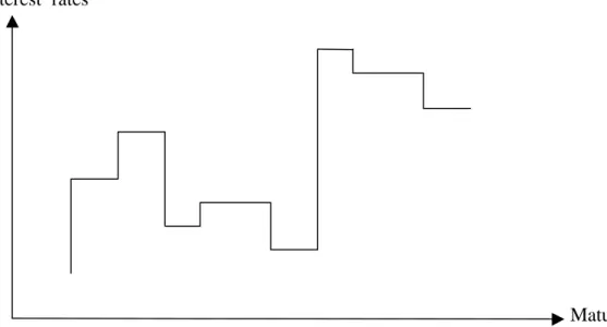
Interest rates
Maturities
Fig. 1 Broken line type of yield curve acceptable under the Market Segmentation Hypothesis
If the financial market is somewhat segmented but yet the yield curve is a smooth and trendy line - instead of a broken one - some reasons might be behind that shape. This is the central question that led to this paper.
b) One reason might come from an inter-temporal or inter-maturity form of arbitrage explored by every investor (supplier of funds) and/or by every creditor (borrower of funds). If the rate2 R1 for 1 month is much below R2 for 2 months, an investor might prefer to
extend a bit his deposit to two months in order to benefit from that higher return. The deci-sion to extend or not depends on the comparison between the benefits earned from such extension and the costs imposed by that reduction in his liquidity.
2
We use capital letters to refer to current spot rates and small letters to refer to both future short-term spot rates. Of course R1 = r1.
If that comparison favours the extension, it will be used by a number of other inves-tors, and that shift will reduce the overall supply of funds in the 1 month bracket and will enlarge the supply of funds in the 2 months interval. Rates will be forced down for the later maturity and up for the first, and the difference between the two initial rates will be reduced.
Also borrowers, faced with R1 <<<< R2 might be able to change slightly their
require-ments of funds and raise for 1 month instead of for 2 months. From this demand side, the two rates will also tend to level off, provided the costs of that change of policy is more than compensated by the reduction of the rate from R2 to R1.
In case R1>>>> R2, the suppliers may move funds to the shorter maturity and the
bor-rowers to the longer one until the two rates approach each other, in both cases forcing the two rates to come closer one to the other. Of course, in the real life these two maturities can only be mutual alternatives if they are rather close, which means that, for example, for 1 month and 10 years this logic cannot apply.
c) A similar inter-temporal arbitrage might be explored by those working in the forward market. Once again, if the 2 months rate R2 is somewhat higher than the one month
R1, the implicit rate r2 for the second month is much above R1.
This high appeal of a large return in month two will increase the demand for 1 month borrowed money and enlarge the supply of savings for 2 months deposits, forcing the first rate to go up and the second to go down, until r2 reaches a level low enough to stop
sedu-cing investors to save at a higher rate in the second month. Of course, this deposit shifting is more likely to occur between similar maturities due to the lower costs involved.
Even without a liquid forward market, any investor can capture this rather high for-ward rate by borrowing for 1 month and investing that amount for 2 months, the first month with that loaned money and the second month with his own funds.
Also from the perspective of the borrowers, one might lock in a very low implicit forward rate for the second month by borrowing immediately for two months but making no use of those funds during the first month other than depositing them at the higher rate. Mar-ket forces will once more determine an approach of the two interest rates.
Either way - R1 << R2 or R1>> R2 - the implicit forward rate for the second month
can-not be much different from R1. In these two arbitrage strategies, the higher the costs
incur-red to shift the preferences along the maturity scale, the larger must be the difference be-tween adjacent interest rates to induce a change of attitude by depositors and/or borrowers. So, unless those costs are huge, the forward rate r2 cannot be much different from the
cur-rent short-term rate R1.
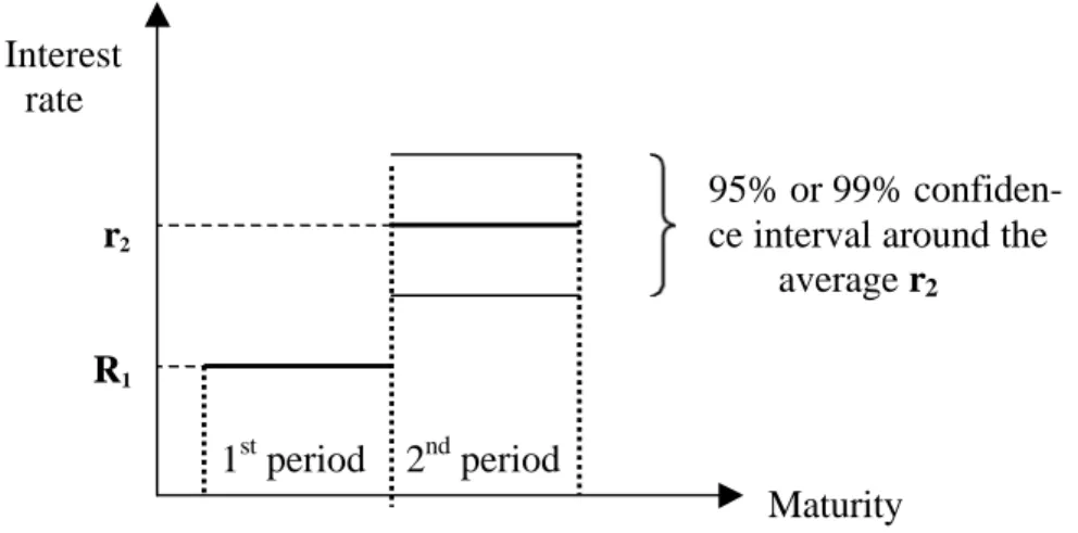
d) Besides arbitrageurs, also speculators are present in this interest rate market. Any-one that wants to deposit for two periods at a known spot rate R2 will consider also the
alternative of starting with a one period deposit (at a known spot rate R1) and risk the level
of the actual return r2 during the second period. The first alternative brings no risk, but the
If depositors forecast higher future interest rates, they may opt for the risky alternati-ve, provided that anticipated improvement is large enough to, most likely, cover the uncer-tainty involved in that estimated (= average) future rate. Here the comparison is between the losses of a lower than expected rate (when the second period starts) and the potential excess return obtained if the personal estimate is correct.
Interest rate
95% or 99%
r2 ce interval around the average r2
R1
1st period 2nd period
Maturity
Fig. 2 A large difference between adjacent rates is not sustainable
On the other side of the fence, if borrowers forecast a large decrease of future inte-rest rates, some of them will similarly prefer to borrow short term - one period only - and risk the future rate for the second period.
In both cases, speculators compare their estimates of future rates to the current for-ward rates implicit in the difference between R1 and R2 spot rates. When the deviation3 of
their estimates from the forward rate is large enough (in the scale of the “normal” volatility of future interest rates), the risky strategy may be selected by some of them. When that deviation is small, the guarantied strategy will be opted for.
Confidence
Estimated rate interval
Forward
Fig. 3 The largest probability is that the future actual rate will be above the forward rate
Here risk is measured by the probability that each one´s estimate of r2 is sufficiently
above or sufficiently below the implicit forward rate to make negligible the odds of a loss in comparison to the non-risky strategy (using directly or indirectly the forward rate).
3
Notice that, in the case of a shift in the supply of funds from 2 periods to 1 period to explore a larger forward rate, because the estimated future rate is larger then the implicit forward rate, market forces will push R2 upwards and R1 downwards, in both cases
enlar-ging the forward rate r2 and, therefore, reducing the incentive for that speculative strategy.
In fact, after these adjustments, the probability to earn an extra return with the risky option will be much smaller. Similarly for a shift from 2 period borrowings to 1 period loans to pay much less interests in the second period.
What the action of these speculators show is that implicit forward rates and estima-ted future spot rates cannot deviate much one from another.
e) Since all these three arguments indicates that r2 cannot be much different from R1,
also R2 cannot be much different from R1, a fact that actual yield curves seem to fulfil. So
this logic suggests that, for short term loans and deposits – say, some days, a few weeks or one or two months – the current spot rate r1 = R1 must determine most of the expected value
of the future spot rate r2 valid for an equal term starting after the end of first one.
R1 r2
Fig. 4 Current spot rate R1 determines most of the adjacent future spot rate r2
Hence, accepting the EH and assuming a linear model for simplicity sake, one is led to write that r2 =a+b.r1. However, this gives only an average of the estimated future value
r2 since the costs of arbitraging or the risks of speculation introduce a certain margin of
un-certainty around that centre value obtained from r1. That is, r2 has some "noise" attached to
it and that is expressed by an additional random term εε2
2 1 2
=
a
+
b
.
r
+
ε
r
According to this logic - r1 determines most of the value of r2 - the parameter b must
be smaller than 1, but rather close to unity, and the parameter a must appear in the formula to complement the result of the product b.r1 and make r2 either larger or smaller than r1
depending on the market views for the future:
a > (1 – b ). r1 means a trend towards larger rates in the future
a < (1 – b ). r1 means a trend towards smaller rates in the future
The error εε2 might follow any kind of distribution with zero mean, but it will be
[ ]
22
,
σ
ε
=
N
o
The shortest time interval in current money markets comes from overnight deposits and loans. So the most detailed model uses rates for 24 hours loans and deposits.
This model fits well into the EH since it explains the shape of the yield curve as the result of the current set of estimates for the future short term spot rates. However, nothing has yet been said about any potential risk premium included in the current long-term spot rates. So, for the moment, forward rates are non-biased estimates of future spot rates.
4. The basic model 4.1. Extension to n periods
In the basic model, the overnight rate r2 estimated for tomorrow is determined by
to-day’s 24 hours spot rate r1 according to parameters a and b, but there remains some
uncer-tainty εε2 in this forecast due to some superimposed “noise”. For simplicity sake, this random
variable is assumed to follow a Gaussian distribution with variance σσ2.
For the day after tomorrow, the same arbitrage/speculation mechanisms determine also that r3=c+d.r2+ε3 and the question is whether a = c, b = d and whether εε3 follows
the same distribution as εε2. Probably the market agents that operate between days 2 and 3
are not exactly the same that operate between days 1 and 2, and that means that the 3 para-meters might change along the yield curve. However, one can simplify the analysis by wor-king with some average values common to all periods4.
So, maintaining the parameters for the day after tomorrow, the current estimate for the correspondent overnight rate is
3 2 3
=
a
+
b
.
r
+
ε
r
which leads to ) . ( . ) 1 .( 2 1 3 2 3 a b b r ε bε r = + + + +and for day n
4
4
4
4
4
4
3
4
4
4
4
4
4
2
1
,)
.
...
.
.
(
.
)
...
1
.(
2 2 1 1 1 2 2 2 2 n n n n n n n na
b
b
b
b
r
b
b
b
r
εε
ε
ε
ε
− − − − −+
+
+
+
+
+
+
+
+
+
=
4Even assuming that all εεi follow the same Gaussian distribution with the same variance σσ2, each disturbance
Noting that the multiplier of a is a geometric progression and denoting by
ε
n, the added noise term, 1 1 1 . 1 1 . n n n n b r b b a r + + ε − − = − −
This expression gives the future overnight term rate rn decomposed into 3 parts:
• since 0 < b < 1, the first term on right (in a)increases with n and tends to an asymptotic long-term value
r a
b
= − 1
• the second term (in r1) decreases with n and becomes negligible for distant future
dates (large n): today´s short-term rate does not influence the long future
• the noise term is a linear combination of the successive disturbances embedded in each estimated value ri before and up to rn; since it seems reasonable to accept
that εεi is i.i.d. 5
5
There is no reason to suspect that the noise term εεi included in the forecast of ri (based on ri-1) should depend
upon any previous disturbance εεi-k. Any of these terms simply translate the local impact of the diversity of
costs among speculators and/or arbitrageurs. Therefore, one might simplify the analysis and accept that all εεi
follow the same statistical distribution (same σσ) and that each one is independent from any other.
BASIC YIELD CURVE MODEL FUTURE ESTIMATED OVERNIGHT RATES
2,5% 3,5% 4,5% 5,5% 6,5% 7,5% 8,5% 0 50 100 150 200 250 300 Number of Days
Interest rates (annualized)
[ ]
≠ = j i for 0 j = i for , 2 σ ε εi j Ethat combination still follows a Gaussian distribution6
− − − 2 1 2 2 , 1 ) ( 1 . , 0 ~ b b N n n σ ε
This shows that the uncertainty of rn grows the further one looks into the future, but
with an asymptotic maximum given by σσ2/(1-b2).
1.2. Interpretation of the parameters of the model
The long term rate r is the level of overnight rates estimated for dates far away into the future. It is an average value that suffers the effect of an additive noise εn, that may deviate the actual rate from that estimated average.
Parameter b indicates how much of r1 is included in r2, but the expression for r2 can
be rewritten in a different way
b r r r r r b r r2 = 1+(1− ).( − 1)+ε2 = 1+η.( − 1)+ε2 with η =1− 6
See annex for derivation of the variance of this noise as seen from today.
BASIC MODEL. FUTURE OVERNIGHT RATES
Confidence interval due to the presence of "noise"
2,5% 3,5% 4,5% 5,5% 6,5% 7,5% 8,5% 9,5% 0 50 100 150 200 250 300 Number of days
Interest rates (annualized)
Future expected overnight rate Average + 1 Standard deviation Average - 1 Standard deviation Long term trend of overnight rates
which makes clear that η η indicates how much of the difference between the current over-night rate r1 and the long term 24 hours rate r is covered during the first day.
And since η% of that difference is “jumped” in the first day, the entire transition from r1 to r would be covered in ττ = 1/η days should that first “velocity” be maintained
unchanged in the fol-lowing days. Of course, the more b approaches 1 the less r2 can be
different from r1 and the slower will be the transition from r1 to r .
We see that this model is completely defined by the following 3 parameters (the noi-se component requires a fourth parameter7, the volatility σσ):
• initial or current overnight rate r1
• long term estimated overnight rate r
• transition time ττ (in our case, days) between r1 and r .
, 1 1
)
.(
)
1
(
n n nr
r
r
r
=
+
−
η
−−
+
ε
or better , 1 1)
.(
)
1
1
(
n n nr
r
r
r
ε
τ
−
+
−
+
=
− with
−
=
=
=
−
=
b
a
b
a
r
1
1
1
1
η
τ
η
7Below it is found that a 5th parameter (k) might be necessary in connection with this noise factor.
BASIC YIELD CURVE MODEL
Transition time to the long term overnight rates
2,5% 3,5% 4,5% 5,5% 6,5% 7,5% 8,5% 0 50 100 150 200 250 300 Number of days
Interest rates (annualised)
1/ηη
1.3. Estimated spot rates
For a low level of annual interest rates - say 3% or 5% - the correspondent daily rates are always very small numerical figures. This allows a simplification when compounding the estimated future overnight rates to obtain the estimated spot rates appropriate for each particular maturity. If fact, for two days, the spot rate is
2 ) 1 ).( 1 ( 1+R2 = +r1 +r2 ⇒ R2 ≅ r1 +r2
and, for three days, is
3 ) 1 ).( 1 ).( 1 ( 1 1 2 3 3 3 3 2 1 3 r r r R r r r R = + + + ⇒ ≅ + + +
Adopting this linear aproximation, the estimated 4 days spot rate is given by
+ + + + + + + + + + + + + + + = . ( . ) .(1 ) . ( . ) .(1 ) . ( . . ) 4 1 4 3 2 2 2 3 4 1 3 2 2 3 1 2 2 1 1 4 14 24 4 34 1444442444443 14444444244444443 r r r b b r b b b a b r b b a r b a r R ε ε ε ε ε ε
and rearranging the terms
[
]
[
]
{
.
1
(
1
)
(
1
)
(
1
).
.(
1
)
.(
1
)
}
4
1
2 2 3 4 1 3 2 2 4a
b
b
b
b
b
b
r
b
b
b
R
=
+
+
+
+
+
+
+
+
+
+
ε
+
ε
+
+
ε
+
+
This expression helps in writing the formula for the n period spot rate Rn
BASIC MODEL. FUTURE AND SPOT RATES
2,5% 3,5% 4,5% 5,5% 6,5% 7,5% 0 50 100 150 200 250 300 Number of days
Interest rates (anualized)
Expected future overnight rates Long term trend of overnight rates Current spot rates
[
]
[
]
+ + + + + + + + + + + + + + + + + + + + = ∑ = − − − − 4 4 4 4 4 4 4 4 3 4 4 4 4 4 4 4 4 2 1 L L L L L , , ) 1 .( ) 1 .( ). 1 ( ) 1 ( ) 1 ( 1 . . 1 1 2 2 1 1 1 2 1 n n n n n n n i n b b b r b b b b b a n r n R ε ε ε εNoting the presence of a number of geometric progressions, the above formula for the n period spot rate can be simplified8 to
,, 1 1 . 1 1 . 1 1 1 . 1 . 1 n n n n r b b n b b n b n n b a R +ε − − + − − − − − = −
or, using the parameters r , r1 and ττ
, , 1
)
1
1
(
1
).
.(
n n nr
r
n
r
R
ε
τ
τ
+
−
−
−
+
=
where the noise component still follows a Gaussian distribution
− − + − − − − − − − 2 ) 1 .( 2 2 1 2 2 2 , , 1 1 . 1 1 . 2 ) 1 ( ) 1 .( , 0 ~ b b b b b b n b n N n n n σ ε
These two formulae indicate that:
• the yield curve (spot rates) evolves upwards or downwards with n depending on the relationship between the initial overnight rate r1 and the long term rate r but,
in any case, it evolves monotonically to
r
a
b
=
−
1
• the variance of the noise term εn,, also depends on n and although it might "ho-ver" above σσ22 for a small number of days, in the long run, it tends to decrease9 due to the normal averaging effect of the successive overnight rates that are added up to obtain the long term spot rate.
8
See the derivation in the Annex.
9
It is curious to note that although rn suffers for increasing uncertainty when n
increa-ses, the error of Rn decreases with n. That is, the market forecasts better a long term spot
rate than medium term spot rates.
4.4. Double regime (two different set of parameters)
Some times the market may estimate an increase in the rates in the near future that are to be followed by some reduction to more modest rates some time after. The yield curve will then start with a positive slope to inflect downwards somewhere in the future to approach smaller levels of interest rates. Other situations show the opposite, that is, an initial negative slope followed by an inversion to a positive one.
VARIANCE OF CUMULATED "NOISE"
Assumed independent from day to day
0 0,5 1 1,5 2 2,5 3 0 200 400 600 800 1000 1200 Number of days b = 0,97
A MODEL FOR THE YIELD CURVE
A regime with two long term overnight rates
2,5% 3,0% 3,5% 4,0% 4,5% 5,0% 5,5% 1 21 41 61 81 101 121 141 161 181 201 221 241 261 281 Num b e r o f d a y s
Interest rates (annualised)
Estimated future overnight rates Current spot w ithout liquidity premium Current spot rates w ith liquidity premium Long term overnight rates
The model can approximate such shapes by assuming the existence of two “long” term levels for the overnight rates - r1 and r2 - and two transition times - ττ1 and ττ2:
• the first n periods are characterised by, r1, a1 and b1 so that the future spot overnight rates
are determined by , 1 1 1 1 1 1 1 . 1 1 . n n n n b r b b a r + +ε − − = − − where − = − = 1 1 1 1 1 1 1 1 b b a r τ
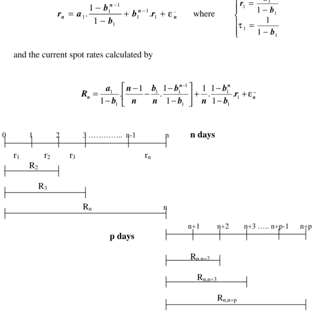
and the current spot rates calculated by
, , 1 1 1 1 1 1 1 1 1 . 1 1 . 1 1 1 . 1 . 1 n n n n r b b n b b n b n n b a R +ε − − + − − − − − = − 0 1 2 3 ………….. n-1 n n days r1 r2 r3 rn R2 R3 Rn n n+1 n+2 n+3 ….. n+p-1 n+p p days Rn.n+2 Rn,n+3 Rn,n+p
Fig 5. Double regime model
• and the second group of p days is characterised by parameters rn+1, a2 and b2 where rn+1
plays here the role of r1
noise . 1 1 . 2 1 1 2 1 2 2 − + + − = − − + + n p p p n b r b b a r where − = − = 2 2 2 2 2 1 1 1 b b a r τ
To calculate the spot rates for maturities falling into this second regime, the simplest approach is to use the arithmetic average of all overnight rates from day 1 until day (n + p).
Beyond r1 ≠ r2 , there is no reason to believe that the two “velocities” of transition
ττ11 and ττ22 should be equal. Therefore, the parameters a and b will probability change from the first set of n days to the second set of p days.
4.5. Liquidity premium
Up to now we have assumed implicitly the Perfect Expectations Hypothesis version of the EH by calculating the current spot rate Rn for n days as the simple average of all the
future overnight rates - from r1 until rn. The increased uncertainty ε of future overnighti, rates ri did not affect the expected value of the long-term spot rate Rn.
However longer term investments impose a loss of liquidity to the creditor which means that to bribe investors into those loans, borrowers need to pay some spread on top of the rate obtained by simply “adding” the successive short term rates forecasted for each future day of that loan.
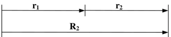
In fact, someone who lends for two periods (R2) faces the uncertainty of the rate in
effect in the second period (r2) should he be forced to liquidate that investment beforehand:
he never knows the market value of his investment when forced to sell. Therefore it is the uncertainty of r2 that somehow will determine that liquidity spread. That uncertainty might
well be found in the standard deviation σσ22 of the noise 2 ,
2 ε
ε = embedded in r2.
A MODEL FOR THE YIELD CURVE A regime with two long term overnight rates
1,5% 2,0% 2,5% 3,0% 3,5% 4,0% 4,5% 1 21 41 61 81 101 121 141 161 181 201 221 241 261 281 Number of days
Interest rates (annualised)
Estimated future overnight rates
Current spot rates w ithout liquidity premium Current spot rates w ith liquidity premium Long term overnight rates
r1 r2
R2
Fig. 6 Comparison between the spot rate for 2 days and the cascaded 2 one day rate
Accepting a linear relation for simplicity sake10
premium p2 = k. σσ
where k is a constant of proportionality dependent upon the more or less intense risk aver-sion of the market players. Therefore, for two days, the spot rate R2 is given by
2 2 1 2 .( ) 2 1 p r r R = + +
For 3 days, there must exist an additional premium p3 (on top of the sum of R2 to r3)
to induce investors to lend money for 3 days (R3) instead of 2+1 days
3 2 3 2 1 3 3 2 3 .( 2. ) 3 1 ) . 2 .( 3 1 p p r r r p r R R = + + = + + + +
where, from the noise of , 3
ε , one can write
4 2 3 . 1 1 . b b k p − − = σ
For n days, the spot rate estimated taking into account the liquidity premium is
n p n p p p n r R n n i premium with n . . 4 . 3 . 2 ) ( =
∑
1 + 2 + 3+ 4 +L+ that is∑
+ = n i premium without n premium with n i p n R R 2 . . 1 ) ( ) ( And since 10) 1 ( 2 2 . 1 1 . − − − = i i b b k p σ
the liquidity premium included in Rn is given by
[
2 4 6 2.( 1)]
2 .2. 1 3. 1 4. 1 . 1 1 . . − − + + − + − + − − = n b n b b b b n k premium σ L4.6. Forward rates for p days
Usually the financial market supplies interest rate data related to the yield curve for a set of maturities, typically weeks, months and/or years. There is not much information for daily maturities. For example, every day Telerate supplies 14 spot rates from the Euro money market:
Eonia 1 W 1 M 2 M 3 M 4 M 5 M
6M 7M 8 M 9 M 10 M 11 M 12 M
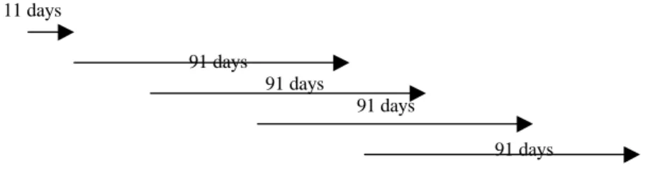
In the case of the Eurodollar futures the market does not supply a set of spot rates but rather a collection of forward rates. Although all these rates are for deposits lasting 91 days, some future deposits begin while some former ones are still running. There is some overlap-ping of maturates and in particular the first deposit may start less than 91 days ahead of today: 11 days 91 days 91 days 91 days 91 days
Fig 7. Eurodollar Futures and the overlapping of the nominal deposits
To work out these cases where the successive maturities do not differ by one single day there are two alternatives:
a) one uses the numerical expression of the forward rate for an operation lasting p days (p=91 in the case of the eurodollar futures) but starting after n initial days. It requires11 the computation of both rn+1 and Rn,n+p:
, , 91 91 1 91 , ) 1 1 ( 1 . 91 ). ( ε τ τ + − − − + = + + r r r Rnn n
b) the other works with forward rates (for 91 days deposits) obtained from the futures pri-ces as if they were overnight rates ri, that is, the model works with periods of 91 days
instead of 24 hours; all expressions for rn and Rn for the overnight model are used here
assuming that r1 - the rate implicit in the price of the first contract alive - is the current
spot rate for an immediate 91 days operation.
Since the first alternative can best explore the entire set of data obtained from the traded contracts, even those overlapping futures, it is the one recommended.
The above expression of Rn,n+91 can be modified in order to use r1 instead of rn+1:
− − − = − + +91 1 91 , ) 1 1 ( 1 . 91 ). ( τ τ r r r Rnn n n n
r
r
r
r
1(
1).(
1
1
)
τ
−
−
=
−
+which, by simple substitution, yields the desired expression for the forward rate as a func-tion of r1:
−
−
−
−
+
=
+91 1 91 ,)
1
1
(
1
.
91
.
)
1
1
).(
(
τ
τ
τ
n n nr
r
r
R
11Note that in this formula, the total uncertainty of Rn,n+91results from the noise included in rn+1 plus the
5. Applications of the model 5.1. Introduction
The quality of this model can only be gauged by applying it to real market data in order to describe actual term structures by means of a single mathematical formula with 3 parameters. Of course, these parameters must be estimated from that data by the best fitting a curve to the available sampled points.
Unfortunately, the model produces a non-linear function of the maturity i and of ττ and that requires the adjustment to follow a numerical methodology due to the absence of closed form equations for those 3 parameters. However, simply minimising the root mean square of the deviations between the curve and the observed points is not enough as it is also necessary to force the average error to be zero12:
• Min
∑
(Ri −Rˆi)2•
∑
(Ri −Rˆi)=0For that purpose, a number of examples were used: Lisbor, Euribor, Euro$, US T-Bills, US Strips.
5.2. Margin of error of the estimated parameters
The quality of the fit can be measured by the non-linear ratio R2 defined as
∑
∑
− − = 2 2 2 ) ( ) ( 1 R R error R i iOne could also proceed and compute the margin of error of the estimated values obtained for the 3 parameters. But the calculation of the standard error of each of those 3 estimates implies overcoming two barriers:
• the model is non-linear in one of the parameters13 (τ) although it may look linear in the two other parameters
12
This null condition for the average error is required to be consistent with the basic model where [ ]i = 0
E ε , and therefore also
[ ]
, = 0i E ε and
[ ]
,, = 0 i E ε . 13 one term long the to rate current from time transition 1 1 rate overnight term long 1 rate overnight current 1 1 b b a r R r − = − = = = τ, , 1 , , 1 ) ( ). 1 1 ( 1 . ). ( i i i i F i i R r r r F i r r r R i ε ε τ τ + ⇒ = + − + − − − + = 4 4 8 4 4 7 6 • the disturbances ,, i
ε are heteroskesdastic and very much auto-correlated
[
]
0 1 ) ( 1 . 1 1 ). 1 .( ) 1 ( . ) 1 ).( .( ; 2 1 2 2 1 2 2 ,, ,, ≠ − − + − − + − − − − − = −− − − − b b b b b b b k n b k n n Cov k n k n k k n n σ ε εIn addition, not always this simple model is recommended to best describe the sam-pled points. Sometimes, market data suggests the use of a double regime model where, besi-des two sets of parameters, one also has also to estimate the transition moment from one regime to the next. Also for cases with very long-term data (e.g. 30 years) the use of the ver-sion with a liquidity premium to better estimate the asymptotic rate r turns the computation into a practically intractable task. In all these cases the ratio R2 can always be directly cal-culated, but it is much more time consuming to compute the standard error of every para-meter. Therefore, in this first approach, the quality of the fit was restricted to the ratio R2.
In all cases the adjustment of the curve to the sampled points was obtained via a trial and error method based on the "solver" instruction of the Excel language.
5.3. Some typical cases
The following examples provide a first measure of the quality of this model by esti-mating the parameters for different countries and for different segments of the term structu-re. In all of them the quality of the fit appears to be rather high, but one must not forget that the yield data used came from basically "one single picture" of the world of interest rates where all samples were collected almost at the same time. Mind also that national markets are increasingly interconnected which is relevant when the time frame is short.
a) Eonia and Euribor14
In Euroland, these rates are a daily measure of the short-term part of the interest rate market (up to 12 months). Due to the precautions taken against the Y2K bug, the yield curve has been showing a distortion for the two standard maturities that settle just before and just after the end of the year (1999). December 29 was the first day without the presence of that non-recurrent disturbance at any point along the curve.
14
Source of data: Internet page "Reference Interest Rates of the EURO area´s Money Market" from Banco de Portugal. Eonia rate is calculated by ECB and all Euribor rates are calculated by Bridge-Telerate.
This is the single case where the market provides direct information about the value of r1 leaving as unknowns only r and ττ. This enabled to adjust a curve either forcing r1 to
be equal to Eonia or leaving this variable free. The 14 maturities lead to the following para-meters of the curve:
EURIBOR & EONIA
29-Dec-99 r1 r ττ R
2
Without Liquidity Premium
Estimated Average 3,080% 5,145% 359 days 0,996
Est. Value with r1 = Eonia 3,040% 4,619% 221 days 0,991
With Liquidity Premium
Estimated Value 3,080% 5,146% 359 days 0,996
Est. Value with r1 = Eonia 3,040% 4,609% 220 days 0,991
Introducing the liquidity premium does not change visibly the quality of the fit due to the short maturities involved where that premium still does not show its effects. The two different fitted curves are so similar that the graph has the two curves completely overlap-ping. Refer to the Annex for the complete data, the adjusted curve and the summary of the calculations.
b) The French Capital Market15
The French government debt market is one of the largest in Euroland and so much so that it can be assumed that any liquidity factors that might exist do not disturb heavily the level of the different interest rates. It also trades debt instruments with very large maturities (up to 30 years). Data from the available 15 maturities (no overnight rate) is published by the French Treasury and the parameters of the fitted curve are the following:
FRENCH TREASURIES
30-Nov-99 r1 r ττ R
2
Without Liquidity Premium
Estimated Average 2,795% 5,897% 811 days 0,979
With Liquidity Premium
Estimated Value 2,755% 5,662% 695 days 0,983
Here the introduction of the liquidity premium - k.σ = 0,00085% p.a. - improves slightly the quality of the adjustment and reduces the spread between r1 and r . Refer to the
Annex for the complete data, the adjusted curve and a summary of the calculations.
15
c) The USA Capital Market (Strips)16
The use of the strip market allows one to work directly with spot rates (not YTM ra-tes from bonds) and also supplies a large sample (60 points). In order to minimise the impact of any potential liquidity effects upon the market rates, only those strips produced by bond and note principals were considered17. This might be particularly relevant for very long ma-turites were tradability tends to dry out.
AMERICAN STRIPS
Notes and Bonds Principal only
01-Dec-99 Without Liquidity Premium R2 = 0,922
First regime r1
r
1 ττ1Estimated Average 5,480% 6,967% 948 days
Second regime rn+1
r
2 ττ2Estimated Average 6,963%18 5,125% 2 372 days
Here a curve generated by two sets of parameters (double regime) was adjusted to the sample with a crossover between Feb 2015 and Aug 2015. Refer to the Annex for the complete data, the adjusted curve and a summary of the calculations.
d) Eurodollar Futures19
The market here does not supply a set of spot interest rates but rather a collection of future rates for 91 days deposits starting at the end of the future contacts. Therefore one has to work with an adapted formula of the model:
− − − − + = +91 1 91 , ) 1 1 ( 1 . 91 . ) 1 1 ).( ( τ τ τ n n n r r r R
where r is the long run overnight spot rate, r1 is the current overnight rate, ττ is the
transi-tion time and Rn,n+91 is the current future rate for a deposit that will start on the day n+1.
The advantage of the Eurodollar futures is the large number of contracts open for tra-ding at any time. One gains access to a large sample of interest rates for maturites up to 10 years ahead.
16
Source of data: "U.S. Government Strips" published in the issue of the Wall Street Journal Europe of Satur-day, 3 - 4 December 1999.
17
Mind that strips from coupons tend to be less tradable than the strips from principals due to their small out-standing nominal amounts.
18
This is an approximation by taking as rn+1 the last overnight rate rn from the initial regime.
19
EURODOLLAR FUTURE CONTRACT
8-Jul-99 r1 r ττ
Without Liquidity Premium R2 = 0,961
Estimated Average 5,400% 7,650% 1 464 days
Refer to the Annex for the complete data, the adjusted curve and a summary of the calculations.
6. Conclusions
The basic idea that the current short term spot rate (for one day, one week or so) must determine most of the value of the next period´s rate seems to be powerful enough to produce a rather flexible building block. Armed with it and combining it in different ways, one can construct an equation that not only describes the general shape of the yield curve but can also be calibrated to fit the actual rates sampled from the market via different financial instruments. In fact, in all the few examples tested the model led to curves that run very close to the sampled points as one can gauge by the very high R2 values obtained.
That basic model has three quantitative parameters to be estimated from market data, all of which have an economic interpretation:
• r1: the current short term rate (typically, the overnight rate)
• r : the asymptotic future level of that short term rate (in the long run)
• ττ: the “velocity” of transition from the current rate r1 to that future level r of
inte-rests and which is expressed by the number of days required to “complete” that jump.
Additionally and from a pragmatic point of view, the last two parameters may help in two areas:
• ττ is a quantitative measure of the expectations of the market about the proximity of a future change in the short term level of interest rates; this is a relevant infor-mation when the monetary policy conducted by a central bank is based on a short term target rate that is continuously steered by that bank; in particular, modifica-tions in the size of ττ indicate the imminence or not of a jump in that target rate;
• as a future short-term rate, r is a more explicit information about the future level of interest rates than the traditional long-term spot rates since these last ones are a mixture of the rates expected to exist from today until that long period; additio-nally, the introduction of the liquidity premium allows to obtain an interest rate r completely clean from that premium and so closer to the expected overnight rate. The model is also very flexible in the sense that it can be adapted:
• to describe regimes with only one set of parameters - positive or negative slope term structures - along with regimes with two sets of parameters - initial positive slope followed by an inversion on that derivative of the curve and vice-versa;
• to adjust curves to market data produced by different financial instruments: a col-lection of spot rates, a set of eurodollar futures prices, etc20;
• to estimate, without interpolation, the interest rates for non-standard maturities. It is likely that the model can be improved by adding a liquidity premium which is solely dependent upon the maturities of the interest rates. That requires the introduction of 2 additional parameters, but the main drawback of that improvement is the increased mathe-matical sophistication required in any practical use of the model. Besides, it is not yet clear that the higher quality of the adjustments with that premium compensates for the added work required to adjust the curve to any sample of points. In particular, it makes almost impractical to calculate the standard deviations of the parameters of the model.
The model draws heavily from the Expectation Hypothesis and is also improved by the addition of a concrete form of the liquidity premium. In that sense the model will be supportive of both the expectation and liquidity premium hypothesis if the high quality of the fits encountered now can be confirmed with further examples of the term structure.
In fact one cannot forget that all the examples tested in this paper came from a rather narrow set of cases where the different markets were very much interconnected - all the yield curves might be similar due to intense relationship of their markets - and also that all of the them were taken from a rather short time interval - the yield curves did not show pro-nounced changes in their basic shapes along that time window. Only future samples will provide significantly different curves to test more thoroughly this model.
This test of time is particularly necessary for the improved version with the liquidity premium added. First, because such a premium can only play a significant role for long ma-turities, suggesting further tests using long term data. Second, because all the curves used followed rather simple shapes and that has very much contributed to the high quality of the fittings encountered. With very high R2 values obtained without that premium, any improve-ments brought about by the introduction of that sophistication may not be very significant, if useful at all.
Finally, another test to the model might come from the margin of errors of the esti-mates of the 3 parameters: how much accurate are the estiesti-mates obtained from real data ?
7. References
• Balduzzi, P., Bertola, G. and Foresi, S., "A model of Target Changes and the Term
Structure of Interest Rates", Journal of Monetary Economics 39, 223 - 249, 1993. • Balduzzi, P., Bertola, G., Foresi, S. and Klapper, L., "Interest Rate Targeting and the
Dynamics of Short-term Rates", Journal of Money, Credit and Banking 30:1, 26 - 50,
1998.
• Culbertson, J. M., “The Term Structure of Interest Rates”, The Quarterly Journal of
Economics, November 1957, 485 - 517.
20
For example, one can develop mathematical expressions for the discount factors used to value coupon bonds and estimate the 3 parameters that minimise the errors to the market prices of a portfolio of those bonds.
• Cuthbertson, K., "Quantitative Finance Economics. Stocks, Bonds and Foreign
Exchange", John Wiley Series in Financial Economics and Quantitative Analysis,
reprinted Aug 1997.
• Fisher, I., “The Theory of Interest”, Augustus M. Kelley, New York, 1965 (reprint from the 1930 edition).
• Greene, W. H., "Econometric Analysis", MacMillan, 1993.
• Griffiths, W. E., Hill, R. C. and Judge, G. G., "Learning and Practicing Econometrics", John Wiley & Sons, 1993.
• Hicks, L. “Value and Capital”, Oxford University Press, 1939.
• Jääskelä, J. and Vilmunen, J., “Anticipated Monetary Policy and the Dynamic
Beha-viour of the Term Structure of Interest Rates”, Bank of Finland Discussion Papers nº
12/99, September 1999.
• Lutz, F. “The Term Structure of Interest Rates”, The Quarterly Journal of Economics, November 1940, 33 - 63.
• Mankin, N.G. and Miron, J. A., "The Changing Behaviour of the Term Structure of
ANNEX
1. Sum of the first n terms of a Geometric Progression
A formula for the following sum of n terms can be obtained
4
4
4
3
4
4
4
2
1
terms n n nb
b
b
S
1 2....
1
+
+
+
+
−=
by noting that + + + = + + + + = − n n n n b b b b S b b b b S .... . .... 1 3 2 1 2 b.Sn −Sn =bn−1and the final result is
b
b
S
n n−
−
=
1
1
Note that the power of b in the numerator is the number n of terms in the sum.
2. Uncertainty of rn
Summing the contribution of the n first days (n-1 terms) for the total “noise” of rn:
2 2 2 2 1 ,
.
....
.
.
ε
ε
ε
ε
ε
− − −+
+
+
+
=
n n n n nb
b
b
Assuming that the noise of each overnight rate rn is independent from all the others and
that the Gaussian distribution is stable (one single standard deviation common to all days)
[ ]
[
]
2 1 2 2 ) 2 ( 2 4 2 2 2 2 ) 2 ( 2 2 2 4 2 1 2 2 , 1 ) ( 1 . ... 1 . . ... . . b b b b b b b b Var n n n n n n n − − = + + + + = + + + + = − − − − − σ σ σ σ σ σ εand finally
[ ]
2 1 2 2 ,1
)
(
1
.
b
b
Var
n n−
−
=
σ
−ε
3. Term in “a” in the spot rate Rn
This term is the sum of n-1 terms
)
...
1
.(
...
)
1
.(
)
1
.(
+
+
+
+
2+
+
+
+
2+
+
−2+
=
nb
b
b
a
b
b
a
b
a
a
S
and noting that
b
b
b
b
b
b
b
b
b
b
b
b
n n−
−
=
+
+
+
+
−
−
=
+
+
−
−
=
+
− −1
1
...
1
1
1
1
1
1
1
1 2 2 3 2 2L
it can be written − + + − + − + − − − + + − + − + − = − − + + − − + − − + − − = − − − b b b b b b b b a b b b b a b b b b b b b b a S n terms n n 1 ... 1 1 1 . 1 1 ... 1 1 1 1 1 1 . 1 1 ... 1 1 1 1 1 1 . 1 3 2 1 1 3 2 4 4 4 4 4 4 3 4 4 4 4 4 4 2 1 and finally − − − = b b b a n 1 1 ) 1 . . 14. Uncertainty of the spot rate R
The “noise” in the spot rate for n
[
]
− − + + − − + − − = + + + + + + + = − − − − b b b b b b n b b b n n n n n n n 1 1 . .... 1 1 . 1 1 . . 1 ) .... 1 .( .... ) 1 .( . 1 1 2 2 1 2 2 1 , , n ε ε ε ε ε ε εwhich still is a Gaussian distribution with variance given by
[ ]
[
]
[
( 1) 2 .(1 ... ) ( .... )]
. ) 1 .( ) 1 ( ... ) 1 ( ) 1 ( ) 1 ( . ) 1 .( ) 1 ( 2 6 4 2 2 3 2 2 2 2 1 2 1 2 3 2 2 2 2 2 2 ,, − − − − + + + + + + + + + + − − − = − + + − + − + − − = n n n n n b b b b b b b b b n b n b b b b b n Var σ σ ε 4 4 4 4 4 4 4 4 4 8 4 4 4 4 4 4 4 4 4 7 6 and finally[ ]
− − + − − − − − = = − 2 2(2−1) 1 2 2 2 2 ,, 1 1 . 1 1 . 2 ) 1 ( . ) 1 .( b b b b b b n b n Var n n R n n σ σ ε 5. Covariance between ,, n ε and ,, k n− εUsing matrix notation, one can write that the noise for two terms in n and in n-k are:
− − − − − = − − − − = − − − − − − − − ) 1 .( ) 1 .( ) 1 .( . ) 1 ).( ( 1 ) 1 .( ) 1 .( ) 1 .( . ) 1 .( 1 1 2 2 1 , , 1 2 2 1 , , k n k n k n k n n n n n b b b b k n b b b b n ε ε ε ε ε ε ε ε