Efficiency analysis in german banks : an application of Data Envelopment Analysis for the 2013-2016 period

(1)

Efficiency analysis in German

banks: an application of Data

Envelopment Analysis for the

2013-2016 period

Maria Beatriz Pestana de Andrade

Dissertation written under the supervision of

Professor Diptes Chandrakante Prabhudas Bhimjee

Dissertation submitted in partial fulfilment of the requirements for

the MSc in Finance, at the Universidade Católica Portuguesa,

(2)

(3)

(4)

i CATÓLICA-LISBON School of Business and Economics

Efficiency analysis in German banks: an application of Data

Envelopment Analysis for the 2013-2016 period

by Maria Beatriz Pestana de Andrade

May 2018

Abstract

The present Dissertation’s academic research question addresses the assessment of the relative efficiency of German banks for the 2013-2016 period. In order to address the latter research question, this document’s empirical research strategy essentially employs a two-step approach. It first uses an established methodology, entitled Data Envelopment Analysis (D.E.A.), producing a set of baseline findings associated with the efficient measurement of German banking efficiency for the said period. Second, it subsequently employs a robustness check, through the estimation of the Malmquist Productivity Index, in order to extend the critical baseline analysis to an intertemporal framework. The overall findings reflect a proficient and stable assessment of relative efficiency measurement for the German banking industry as a whole (as represented by the chosen sample), by accurately identifying any potential inefficiency sources, which can be potentially improved upon. The banking data were extracted from ORBIS® BankFocus. The inputs considered are deposits and interest expense, while the outputs are loans and interest income. These inputs and outputs were analysed both separately and simultaneously, according to three different approaches: i) deposits and interest expense to loans and interest income; ii) deposits to loans; and iii) interest expense to interest income. An output-oriented approach was also conducted, as model applications test the maximization of outputs for a given level of inputs. Lastly, both constant and variable returns to scale assumptions were addressed in the present Dissertation. The present Dissertation’s overall findings associated with the efficiency measurement related to the performance of the German banking industry are quite stable across the different model applications, notwithstanding some minor expected differences according to the set of model inputs/outputs chosen. This stability also suggests that some banks are more revenue-oriented, while others are more asset-oriented. It is hoped that the findings might contribute to the performance improvement of the Euro Area’s most powerful banking industry.

Keywords: German Banks, Efficiency Measurement, Data Envelopment Analysis,

Malmquist Productivity Index, Relative efficiency, Bank Performance

(5)

ii CATÓLICA-LISBON School of Business and Economics

Efficiency analysis in German banks: an application of Data

Envelopment Analysis for the 2013-2016 period

by Maria Beatriz Pestana de Andrade

May 2018

Resumo

A presente Dissertação aborda como questão científica de partida a eficiência relativa dos bancos Alemães, no contexto do período 2013-2016. A questão científica de partida que preside à presente Dissertação é respondida em duas etapas. A primeira etapa consiste na aplicação da metodologia ‘Data Envelopment Analysis’ (D.E.A.), produzindo um conjunto de resultados de base associados à aferição da eficiência da banca Alemã para o período em questão. A segunda etapa consiste na aplicação do ‘Malmquist Productivity

Index’, estendendo os resultados base a uma dimensão intertemporal. Em função da

amostra representativa, os resultados globais relativos à aferição da eficiência da indústria bancária Alemã são muito eficazes e estáveis, identificando potenciais fontes de ineficácia nesta indústria, que podem ser subsequentemente colmatadas. Os dados foram extraídos da base ORBIS® BankFocus. Os inputs considerados são os depósitos e os juros pagos, enquanto que os outputs são os empréstimos e os juros auferidos. Ambos os inputs e outputs foram analisados quer simultaneamente, quer separadamente, de acordo com três abordagens distintas: i) depósitos e juros pagos relativamente aos empréstimos e juros recebidos; ii) depósitos relativamente a empréstimos; e iii) juros pagos relativamente a juros auferidos. Uma abordagem ‘output-oriented’ foi estimada, de acordo com a qual se procedeu a uma maximização dos outputs face a um determinado nível de inputs. Por último, foram igualmente consideradas as hipóteses ‘constant returns to scale’ e ‘variable

returns to scale’. Os resultados empíricos obtidos referentes à relativa eficiência da banca

Alemã são significativamente estáveis ao longo das diferentes variantes do modelo, não obstante existirem algumas diferenças expectáveis tendo em conta as diferentes combinações de inputs e outputs. Esta estabilidade dos resultados sugere que alguns bancos Alemães são ‘revenue-oriented’, enquanto outros são mais ‘asset-oriented’. Espera-se que a presente análise crítica possa contribuir para a melhoria da performance da indústria bancária da economia mais poderosa da Zona Euro.

Palavras-chave: Bancos Alemães, Aferição da Eficiência, Data Envelopment Analysis,

Índice de Produtividade Malmquist, Eficiência Relativa, Performance dos Bancos

(6)

iii

Table of Figures

Figure 1 - German Banking System ... 10

Figure 2 - Distribution of Landesbanken in Germany ... 11

Figure 3 - German banking structure ... 12

(8)

v

Table of Tables

Table 1 – Summary Statistics – Dataset (Balance Sheet items) ... 10

Table 2 – Summary Statistics – Dataset (Income Statement items) ... 21

Table 3 – D.E.A results Two-output and Two-input model (2016) ... 23

Table 4 – Slack analysis - Two-output and Two-input model (2016) ... 25

Table 5 – D.E.A results One-input (deposits) and One-output (loans) model (2016) ... 26

Table 6 – D.E.A results One-input (interest expense) and One-output (interest received) model (2016) ... 27

Table 7 – D.E.A results Two-output and Two-input model (2013 - 2016) ... 29

Table 8 – D.E.A results Oneinput (deposits) and Oneoutput (loans) model (2013 -2016) ... 30

Table 9 – D.E.A results One-input (interest expense) and One-output (interest received) model (2013 - 2016)... 31

Table 10 – Malmquist T.F.P. Index Components (2013 – 2014) ... 33

Table 11 – Malmquist T.F.P. Index Components (2014 – 2015) ... 34

(9)

vi

Table of Equations

D.E.A generic formulation

Equation (1)……….. 14

Equation (2)……….. 14

Equation (3)……….. 14

D.E.A linear transformation Equation (4)……….. 15

Equation (5)……….. 15

Equation (6)……….. 15

Equation (7)……….. 15

D.E.A input-oriented model Equation (8)……….. 16

Equation (9)……….. 16

Equation (10)……….... 16

Equation (11)……… 16

B.C.C. model (Variable returns to scale) Equation (12)……… 16

D.E.A input-oriented model Equation (14)……… 17

Equation (16)……… 17

Scale efficiency change Equation (18)……… 18

Pure technical efficiency change Equation (19)……… 18

(10)

vii

Glossary

B.C.C. Banker-Charnes-Cooper model. This model considers the variable

returns to scale approach.

C.C.R. Charnes-Cooper-Rhodes model. This model considers the constant

returns to scale approach.

C.R.S. Constant Returns to Scale. D.E.A. Data Envelopment Analysis. D.M.U. Decision Making Unit.

M.P.I. Malmquist Productivity Index. T.F.P Total Factor Productivity. V.R.S. Variable Returns to Scale θ_{/ theta} Efficiency score.

(11)

viii

Acknowledgments

I would like to thank my thesis supervisor, Professor Diptes Bhimjee for all the support during all the dissertation process, from the first steps of this thesis to the final corrections. All the comments were valuable and helped the progression of my work.

I also would like to acknowledge my Professors in this institution, from whom I learnt the topics and work methodology necessary to my thesis elaboration.

Finally, I am very especially grateful to Bernardo Serrão Brochado for all the patience and incommensurable support.

Dedication

For my family: my father Paulo, my mother Isabel, my sisters Júlia and Sofia, my brothers Rafael, Francisco, António and João Paulo and for Bernardo.

Last, but not least, this document and all the effort I put in it is dedicated to God for all the things He gave me (and continues to give). May this be for His greater Glory.

(12)

ix

The greatness of the human being consists in this: that it is capable of the universe.

Saint Thomas Aquinas

De Veritate (On Truth) q. 1, art. 2, ad 4

The empires of the future are the empires of the mind...

(13)

(14)

1

1. Introduction

Efficiency is a widely studied academic research topic in Economics and Finance, since economic agents aim to produce more with a given amount of inputs. However, efficiency can be very difficult to measure, since it is challenging to determine the appropriate measures and approaches to analyze efficiency. Moreover, it is also challenging to find the suitable criteria to quantitatively define efficiency and applying these criteria to various firms and entities.

Banks are one of the most scrutinized institutions by society: customers, politicians, economists, analysts and investors are attentive to their performance due to the high costs of state intervention to rescue banks, when negative externalities arise. That said, every agent of society wants banks to be as efficient as possible, saving resources that can be better used in order to produce more, for instance, to finance the Economy, with the least amount of resources possible. Banks are thus highly complex institutions, and the fundamental aim of this dissertation is to critically analyse banks within an efficiency framework setting.

Accordingly, this dissertation aims to study banking efficiency in Germany, a bank-based economy were banking institutions are essential to the well-functioning of its Economy. More specifically, the present Dissertation focuses on commercial banks, whose principal function is to collect deposits and provide loans, profiting from the interest margin between the interest received from loans and interest paid on deposits.

In order to study this fundamental topic, the present Dissertation employs a sophisticated methodology, entitled Data Envelopment Analysis (D.E.A.). D.E.A. constitutes a non-parametric methodology, initially used in operations research, and subsequently adapted to Finance. Data Envelopment Analysis constitutes a model that measures relative efficiency, thus making a significant contribution to the field of efficiency measurement, thus circumventing the issues on efficiency metrics previously mentioned, since it can be applied to every type of firm, starting from a generic economic efficiency statement. Additionally, the present Dissertation also examines efficiency along a specific timeline, using another model, entitled the Malmquist Productivity Index, thus completing the standard D.E.A. critical analysis, and enriching the present Dissertation. That is, the methodological design covers both a static and a dynamic critical analysis, as well as model applications with robustness checks.

(15)

2 Accordingly, the main academic research question that presides over the present Dissertation addresses the efficiency analysis in German banks for the 2013-2016 period, using the Data Envelopment Analysis Methodology.

Succinctly, our findings suggest that the overall results associated with the efficiency measurement are quite stable across the different model applications presented, even though some minor anticipated changes are observable, according to the inputs/outputs chosen. Moreover, there is some empirical evidence that some banks are more revenue-oriented, whilst others are more asset-oriented.

Lastly, the present Dissertation is structured as follows: section 2 presents the literature review for this research topic, presenting the key concepts related to Data Envelopment Analysis and the evolution observed in the use of this methodology since it was first formulated. Section 3 examines the German banking system, focusing and explaining its peculiar organization. This chapter also briefly analyses the reasons for certain idiosyncratic effects observed in the German banking industry during the financial crises. Section 4 describes the models used in the present Dissertation, namely the Data Envelopment Analysis and the Malmquist Productivity Index; as well as the dataset and corresponding data considerations followed throughout this Dissertation. Section 5 subsequently describes the empirical findings associated with the models’ application for the German banking industry. In this section, three variations of the D.E.A. model are computed and critically scrutinized. The results for 2016 are first analyzed separately, and then the three D.E.A. variations are computed for each year, from 2013 to 2016. Subsequently, the Malmquist Index is also estimated for the period under analysis, allowing for a deeper interpretation of the results within a intertemporal perspective.

(16)

3

2. Literature Review

The present section of the Dissertation critically reviews the most relevant academic literature applicable to the Dissertation’s underlying research question, namely the research topic associated with the empirical measurement of bank efficiency.

Efficiency and, more specifically, bank efficiency, constitutes quite a relevant topic in the academic literature. Berger, Hunter, & Timme (1993) presents an academic survey that critically reviews past academic research of bank efficiency, which, typically, revolves around the analysis of the following research topics: i) scope and scale economies in banking; ii) X-efficiency1_{; iii) bank mergers and its impact on efficiency; iv) the role of}

governmental institutions; and v) efficiency in the insurance sector. The said academic survey concludes by presenting the main drivers of financial institution efficiency. Where the topics of scale and scope economies are concerned, the surveys’ authors suggest that past research demonstrates that the use of translog2_{functions is not appropriate for the}

measurement of efficiency. Instead, the estimation of scale and scope economies should be done on the X-efficient frontier, and both scale and scope efficiencies should be derived from the profit function, in order to fully account for cost and revenue structures. Furthermore, the survey’s authors claim that more research on the concept of financial scale economies is needed, as well as “on the optimal scope economies concept” (Berger, et al., 1993: p. 226).

Farrell (1957) constitutes the first document to present a quantitative method to measure productive efficiency. The author seeks to present a measure of productive efficiency that could be easily applied to any situation where a given set of inputs originate a specific set of outputs. For that purpose, the author observes that the production frontier should be use as benchmark. More importantly, the article presents three measures of efficiency: i) technical efficiency (i.e., inputs needed to produce the observed output versus inputs observed to produce the same level of output); ii) price/allocative efficiency (i.e., costs of producing the observed output at the observed prices versus the costs observed in the efficient frontier); and iii) overall efficiency (“costs of producing the observed output if

1

X-efficiency refers to the amount of outputs necessary to reach the maximum possible for that quantity of input. According to this theory, under perfect competition all firms are x-efficient, because over the long-run x-efficient firms have advantage over the inefficient firms.

2_{It is important to mention the use of translog functions because of their generalized application to the field}

of efficiency measurement, namely to bank efficiency. According to Berger et al.( 1993) these functions are not appropriate when applied to banks of significantly different sizes.

(17)

4 both technical efficiency and price efficiency are assumed relative to observed costs” (Førsund & Sarafoglou, 2005, p. 21)). Moreover, Farrell (1957) illustrates the proposed methodology with an example drawn from agricultural production in the United States of America. Lastly, it should be pointed out that this seminal article’s contribution to the field is twofold: i) it first advances a definition of efficiency measures; ii) it then advances the specification of the production frontier function and its link to efficiency measurement.

The Data Envelopment Analysis (D.E.A.) model was first presented by Charnes, Cooper, & Rhodes (1978) which builds on the previously mentioned document by Farrell (1957). According to these authors, the D.E.A. is essentially a conceptual model that measures decision making efficiency. This model was initially designed to evaluate public programs, more specifically, educational programs. The model states that there are several decision-making units (D.M.U.’s), i.e. entities or firms, with inputs and outputs, and a ‘program’, i.e., a group of decision making units. A ‘program’ can be a set of firms or non-profit entities, for example in the case of the present Dissertation, the ‘program’ is the set of German banks, as shall be seen in subsequent sections. According to the authors, the efficiency determination of a D.M.U. is “the maximum of a ratio of weighted outputs to weighted inputs, subject to the condition that similar ratios for every D.M.U. must be less than or equal to unity” (Charnes et al., 1978, p.430). The weights are not preassigned, but determined using linear programming methods on the data available for each D.M.U. This model is known in the academic literature as the ‘C.C.R. model’. The C.C.R. model was later adapted by Banker, Charnes, & Cooper (1984) in a seminal article addressing this important research topic. The main difference in this framework of analysis is that it accounts for variable returns to scale, whilst the C.C.R. model only considers constant returns to scale. The main drawback of the original model is that the constant returns to scale attribute constitutes an appropriate approach when the D.M.U.s are operating at the optimal level. Otherwise, both technical and scale inefficiencies must be accounted for.

The previously mentioned literature is essentially concerned with the underlying theoretical framework, but the said models were then applied to specific industries and countries, vastly increasing, from an empirical standpoint, the academic literature on this fundamental research topic, thus ultimately originating a great number of empirical

(18)

5

applications (this also coincides with the main focus of the present empirical Dissertation).

The first relevant empirical application of D.E.A. models to the United States of America was implemented by Sherman & Gold (1985). The model was specifically applied to the particular case of a U.S. bank, in order to assess its efficiency. The model was applied to 14 bank branches, the outputs being grouped in four types of transaction types, while the inputs include labour, office space and supply costs. The research findings demonstrate that six out of the fourteen branches were relatively inefficient. Two of the inefficient branches were the smallest in terms of the volume of transactions, which could be justified by the existence of diseconomies of scale, or by the quality of management (assuming that less experienced managers controlled smaller branches.) The authors observed that relatively less efficient branches were near to the contract termination due to the proximity to other branches, and due to low liquidity performance. Additionally, there was a revision of the excess inputs of the non-efficient branches, when a comparison is established between actual input usage and the potential reduction on each input identified with the D.E.A. methodology in order to identify branches that might become more efficient.

Yeh (1996) uses the D.E.A. methodology, alongside with financial ratios, to relate profitability with the financial operating strategies for a given set of banks in Taiwan. The author separates the banks comprised in the sample in three distinct groups – low, medium, and high D.E.A. scores-, while subsequently applying financial ratio accounting for capital adequacy, profitability, asset utilization, and liquidity assessment. The author concludes that, on average, banks with a higher D.E.A. score were less leveraged and “were more aggressive in employing their deposits and assets to generate revenues than those who were less D.E.A. efficient” (Yeh, 1996, p.987). Additionally, the author observed that Taiwanese business cycles, particularly in the 1980’s, were factored in the D.E.A. score. The author also concludes that, with a correct choice of inputs and outputs, the D.E.A. methodology can provide a significant contribution to the evaluation of a given bank’s “financial condition and management performance” (Yeh, 1996, p.988).

Casu & Molyneux (2003) analyze whether the banking industry in Europe faced both improvement and convergence in terms of bank efficiency during the period 1993-1997. The authors used D.E.A. estimation in order to assess the said efficiency. Notwithstanding, it should be noted that the determinants of bank efficiency pose some

(19)

6 issues associated with the dependency of D.E.A. efficient scores, when applied in the context of regression analysis. To overcome this drawback, a bootstrap technique was used by the said research. The authors’ main conclusions suggest that since the EU’s Single Market Program was brought into effect, bank efficiency across the Union improved significantly. However, there is no evidence that convergence amongst countries is observed.

Yue (1992) further evaluates the management performance of 60 commercial banks in Missouri, between 1984 and 1990. For that purpose, the applied methodology used in the article is the C.C.R. model according to the intermediary approach, i.e. financial institutions’ main function is promote the intermediation between savers and borrowers. The outputs adopted were: interest income, non-interest income and total loans; whilst the inputs were: interest expenses, interest expenses, transaction deposits and non-transaction deposits. Yue (1992) performs a window analysis, identifying the relative best and worst banks, as well as the most stable banks.

Analogously, Kocisova (2014) applies the D.E.A. methodology to a set of Slovak and Czech commercial banks, considering the period of 2009-2013. The article aims to compare bank efficiency through either maximizing profit (or revenue), or minimizing costs, thus focusing on revenue, cost and profit efficiency. The methodology used was the input-oriented B.C.C. model (according to the variable returns to scale approach). The variables used to measure efficiency were: total deposits, number of employees, fixed assets, total loans, other earning assets, price of deposits, price of labour, price of physical capital, price of loans, and prices of other earning assets. The findings demonstrate that, on average, banks from both countries increased revenue efficiency; however, Czech banks were the most revenue-efficient, meaning that Slovak banks have more potential to increase revenue efficiency than their Czech counterparts. It should be observed that cost efficiency is reduced in both countries, notwithstanding the fact that it was higher in the Czech Republic. Where profit efficiency is concerned, it decreased in both countries, although being higher in the Czech Republic.

Berg, Førsund, Hjalmarsson, & Suominen (1993) analyzed the efficiency of banks in Finland, Norway and Sweden for 1990. For that purpose, D.E.A. analysis was used, considering both constant and variable returns to scale. The article uses quite a broad data set that includes 503 Finnish banks, 150 Norwegian banks, and 126 Swedish banks. The outputs considered are: total loans (to others than financial institutions), total deposits (to

(20)

7

others than financial institutions), and number of branches. The inputs are labour (measured in man-hours per year), and capital (measured in book value of tangible assets). When performing an individual analysis of the countries comprised in the chosen sample, the authors conclude that Finland and Norway have the largest efficiency spreads. When the analysis addresses the pooled Nordic data set, most banks with the highest efficiency score were Swedish, while one large Finnish bank was amongst the most efficient units, and no large Norwegian bank had an efficiency score higher than 0.9.

Nitoi (2008) examines the efficiency of 15 Romanian banks, comprising around 90% of the total bank assets in Romania in the period of 2006, 2007 and 2008. The analysis was input-oriented, and it focuses on the intermediary approach. The article considered the existence of both variable and constant returns to scale. The outputs were: loans, other earning assets and core operating profit; whereas inputs were deposits and other borrowed funds, number of employees, and number of bank branches; while input costs were: interest expense, personnel expenses, and other administrative and general expenses. In both the constant and variable returns to scale approaches, technical, allocative and cost efficiency were measured. In the case of variable returns to scale, the scale efficiency (ratio between technical efficiency from constant returns to scale and variable returns to scale) was also computed. On the other hand, for the constant returns to scale approach, the total factor productivity (Malmquist Index) was also estimated. The Nitoi (2008) findings demonstrated that large banks were the most scale-efficient, and that banks with Romanian shareholders were the least efficient. Overall, the banks addressed by this study can potentially become more efficient in both allocative and cost terms.

Sahin, Gokdemir, & Ozturk (2016) analysed the Turkish banking system, employing the D.E.A. methodology to examine the effects of the Global Financial Crisis on the country’s banking performance, especially on bank efficiency. The data set is comprised by 19 commercial banks, and the article addresses the period between 2004 and 2012. The article takes into consideration the variable returns to scale input-oriented approach. The input variable set includes: the capital adequacy ratio, deposit rate, liquidity ratio and size of assets; whereas the output set is composed by: quality of assets, loan rate, riskiness ratio, returns on assets rate, shareholder’s equity profitability ratio, and the management effectiveness rate. In order to assess the efficiency of the Turkish banking industry for the time period under analysis, the variance of efficiency scores of the banks was measured using the Malmquist Total Factor Productivity.

(21)

8 In passing, it should be observed that the Malmquist Total Factor Productivity Index is a very relevant metric to compare efficiency in an intertemporal setting, since D.E.A scores provide relative efficiency of a D.M.U in comparison with those of another D.M.U.’s in a certain period – that is, relative efficiency is a static measure. Thus, the Malmquist T.F.P. Index complements a D.E.A score approach, which will be observed in the following sections.

The authors’ findings demonstrate that, on average, efficiency improved between 2006 and 2009, and then decreased in the period between 2010 and 2012. However, if we divide the banks by clusters (i.e., public; private; and foreign ownership), the authors conclude that only the public banks were impacted in terms of efficiency throughout the crisis time frame.

Staub, da Silva e Souza, & Tabak (2010) address the efficiency of Brazil’s banking system using the D.E.A. methodology, thus investigating technical, cost and allocative bank efficiencies for the period between 2000 and 2007. Where the research’s sample size is concerned, the number of banks varied through the years, but was confined to the range between the minimum of 138 and the maximum of 184 financial institutions. Given that the intermediary approach strategy was adopted by the research, the outputs were: total loans net of provision loans, investments, and deposits; while inputs were: operational expenses net of personnel expenses, personnel expenses, and interest rate expenses. The authors’ approach engages a panel data model. This article’s findings suggest that foreign banks are less cost efficient than Brazilian banks, and this conclusion is in line with the home field advantage hypothesis3_._{Additionally, state-owned banks} appear to be more efficient than private institutions, thus rejecting the agency theory

hypothesis4_{. For the 2000-2002 period, the inefficiency of Brazilian banks is more related} to technical inefficiency. In what concerns to size and type of activity, there was no significant evidence supporting differences in terms of bank efficiency.

A critical issue regarding D.E.A. models is the choice of variables. Eskelinen (2017) presents a rigorous research regarding variable selection procedures for data envelopment analysis. The choice of inputs and outputs becomes crucial for the model and, therefore,

3 _{This hypothesis stipulates that domestic companies are more efficient than foreign ones due to}

organizational diseconomies and to regulatory differences (Staub et al., 2010).

4_{According to the agency theory hypothesis, the separation between the interests of ownership and}

(22)

9

sound techniques and approaches are needed to choose inputs and outputs to avoid problems caused by selection bias. The author suggests two methods: i) variable reduction (based on partial covariance); and efficiency contribution measure (based on Data Envelopment Analysis). The variable reduction technique induces variable selection by using a multivariate statistical test (aimed at minimizing the loss of information caused by variable reduction), using as indicator the variance around the mean. While the efficiency contribution measure is based on a process of backward variable elimination. The two methods do not yield the same result, and this fact highlights the need to choose appropriate variables.

(23)

10

3. German Banking System – a brief contextualization

The present section briefly addresses the structure and historical evolution of the German banking industry (sub-section 3.1); while also briefly addressing the impact of the Global Financial Crisis on the German banking industry (sub-section 3.2).

3.1. German Banking System

Germany has a bank-based economy, with banks playing a leading role in the financial system. Germany, alongside with Japan, is the epitome of the bank-based economy (Allen & Gale, 2000).

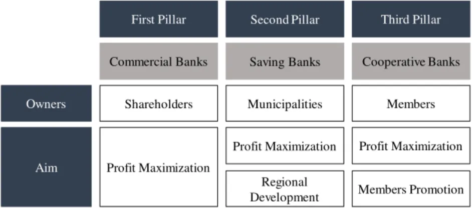
The German banking structure is organized around a three-pillar system, which neatly divides financial institutions into commercial banks5_{, public sector banks and cooperative}

banks. This designation is based on differences in both ownership and activity criteria. The table below summarizes the three-pillar structure in both ownership and aim of activity.

Figure 1: German Banking System

Source: Adapted from Faltermeier (n.d.).

Commercial banks refer to circa 40% of total bank industry, in terms of assets under management, and this segment is composed of: (i) three large groups; (ii) small and medium banks and; (iii) a residual amount of foreign branches. The institutions within

5_{Some authors and institutions (including the I.M.F.) name the first-pillar as ‘private commercial banks’}

(I.M.F , 2011). In the context of the present Dissertation, the term ‘commercial banks’ will be adopted due to the fact that part of Commerzbank (one of the most important commercial banks included in this category) is partially publicly owned, for the period under analysis throughout this Dissertation.

Commercial Banks Saving Banks Cooperative Banks

Shareholders Municipalities Members

Owners

Aim

Profit Maximization Profit Maximization Regional

Development Members Promotion Profit Maximization

(24)

11

this first pillar are both international- and national-oriented. Generally, national-oriented private commercial banks have an inclination to include more specialized services (for example, real-estate related) than foreign banks.

The second pillar consists of public-owned banks, including saving banks (‘Sparkassen’). These banks are also engaged in regional development, although their activities are geographically constrained, while offering a wide variety of products and services to an eclectic group of clients. Sparkassen do not compete with each other, but they do compete with commercial banks and cooperative banks operating in their correspondent region.

Landesbanken were the equivalent of a central bank for the Sparkassen. More recently Landesbanken widened the scope of their activities, engaging in more banking segments

(such as investment banking), hence competing with commercial banks. The figure below illustrates the distribution of Landesbanken across Germany. Figure 2: Distribution of Landesbanken in Germany

Source: Author (2018)

The third pillar is related to cooperative banks. These institutions are large in number, but small with reference to asset size6_{, having quite a relevant presence in rural areas of}

Germany. The ownership of these institutions is peculiar since they are owned by their members, despite being open in the provision of banking services to the general public. They aim to support the financial and economic interests of their members, while taking

6_{According to IMF (2011), cooperative banks account for approximately 65% of the total number of}

(25)

12 advantage of raising funds in a self-sufficient manner as a foremost jointly-owned business. With the openness of cooperatives to non-members, the difference in relation to universal banks activities is less observable.

The figure below describes the current state of the German banking structure, weighted by total assets of each group of banks, with the traditional groups included in the three-pillar designation accounting for circa 80% of the total bank assets. The remaining bank assets refer to a group designated ‘other banks’, including mortgage banks, loan associations, etc. Since this group is quite heterogeneous, it cannot be considered as a fourth pillar.

Figure 3: German banking structure

Source: Deutsche Bundesbank (2018).

The most significant private banks appeared at the end of the 19th_{century. For many}

years, the most important financial institutions within the German Financial system were the following: i) Deutsche Bank, founded in 1870 in Berlin; ii) Commerzbank, also founded in 1870 in Hamburg; and iii) Dresdner Bank7_{, founded one year later in the city}

of Dresdner. Their role was to: i) support the activity of corporations; ii) help the economy; and iii) support the foundation of companies. It was only after the second half of the 20th_{century that these banks opened their operations to the public in general.}

However, some structural changes have occurred in more recent times. For example,

7

Dresdner Bank was acquired by the Commerzbank in 2009 (Financial Times, 2009).

12% 14% 10% 3% 2% 16% 31% 11% 1% 43% Landesbanken Savings banks Cooperative banks Mortgage banks

Building and loan associations Banks with special, development and other central support tasks Big banks

Regional banks and other commercial banks Branches of foreign banks

(26)

13

presently, Dresdner Bank does not exist as a separate bank. Deutsche Bank attempted to acquire it in 2000. Before the international crises, Commerzbank, the third largest commercial bank, acquired Dresdner Bank, the second largest. This acquisition weakened Commerzbank, forcing the German government to rescue it and become its main shareholder (Financial Times, 2009).

3.2. Global Financial Crisis and the German Banking System

Germany was badly hit by the Global Financial Crisis. Hufner (2010) points three main reasons for that: (i) the large amount of toxic assets held by the Landesbanken; (ii) the historical and structural low profitability of its banking system; and (iii) limitations related with banking supervision.

The large amount of toxic assets held by the Landesbanken might be explained by governance shortcomings: these institutions had a guarantee issued by the German government in the event of default of financial products. The European Commission forced the end of these state guarantees, notwithstanding the fact that they were only completely terminated in 2015.

Furthermore, supervision problems were caused by: i) lack of independence of the regulator; ii) narrow focus of the scope of supervision compliance with quantitative requirements only; and iii) limitations associated with macro-prudential analysis.

(27)

14

4. Methodology and Data

The present section succinctly describes the empirical methodology adopted by the present Dissertation (sub-chapter 4.1), as well as the data set herein used (sub-chapter 4.2).

4.1. Methodology - Data Envelopment Analysis

Data Envelopment Analysis (D.E.A.) is a methodology that started to be widely applied in operations research, and then spread out to other research fields (namely to Finance). This methodology is quite proficient in identifying efficient units (entities) and relative efficiencies between the units under analysis.

The Data Envelopment Analysis (D.E.A.) methodology is essentially implemented in two stages: i) it uses the information of the inputs and outputs of each Decision-Making Unit (D.M.U.) to construct the efficient frontier; ii) any subsequent measurement of efficiency is estimated relatively to the efficient frontier.

The original paper by Charnes et al (1978) presents in input-oriented theoretical model, assuming constant returns to scale (C.C.R. model). Later, the initial model was adapted to include other features, such as variable returns to scale (V.R.S.). Banker, Charnes and Cooper (1984) were the first authors to propose the inclusion of variable returns to scale into this specific theoretical framework.

Charnes et al (1978) thus proposes the maximization of the ratio of weighted outputs to weighted inputs for that specific unit, subject to the condition that the ratio be less than or equal to one, and higher or equal than zero. That is:

∑_∑ (1)

Subject to:

0 ≤∑_∑ ≤ 1 ; = 1, 2, …, (2)

(28)

15

Where N is the total number of D.M.U.s, J is the weighted sum of outputs, I is the weighted sum of inputs, M is the base DMU (calculating for the mth _{D.M.U.), N are} D.M.U.’s, I are inputs, J are outputs, are the weights for outputs, and are the weights for inputs.

Please note that the previous model assumes a fractional equation (1), a fact that originates some computational issues in the corresponding estimation, in view of the fact that the objective function is linear. Taking into consideration the existence of non-linearities, Charnes et al (1979) transformed the objective function into a linear form, as stated below: max (4) Subject to: = 1 (5) − ≤ 0 ; = 1, 2, … , (6) , ≥ 0 ; = 1, 2, … , ; = 1, 2, … , (7) The non-negativity conditions ensure that input and output weights will be always positive and the efficiency score will be a number between 0 and 1.

Furthermore, the D.E.A. Charnes-Cooper-Rhodes model has two main variants: i) the output-oriented variant; and ii) the input-oriented variant. The output-oriented model maximizes outputs associated with a given level of input and is stated as the above-mentioned model. On the other hand, the input-oriented model attempts to minimize inputs in order to produce a given level of output. The input-oriented C.C.R. model is also known as the dual model.

(29)

16

min (8)

≥ ; = 1, 2, … , (9)

≤ ; = 1, 2, … , (10)

≥ 0; = 1,2, … , ; free (11)

Where is the efficiency ratio of the mth _{D.M.U. The D.M.U. is relatively efficient if}

its efficiency score ( ) is equal to 1.8

As mentioned before, the C.C.R. model assumes constant returns to scale (C.R.S.). To allow the model to account for variable returns to scale (V.R.S.), Banker et al (1984) adapted the C.C.R. model, adding a measure to capture input excesses and output shortfalls. The model also includes a convexity condition with non-negativity constraints. The model is expressed as:

= ∑ _∑ − (12)

Subject to:

∑ −

∑ < 1 (13)

Where Ek is the efficiency of kth D.M.U., Q stands for output, P for inputs, uj are

weights of output (virtual value), V are the weights of inputs (virtual values), and is a scalar (unconstrained in sign).

8

It is important to mention that a relatively efficient D.M.U. implies a score of 1, but a score of 1 does not imply that the D.M.U. is necessarily in the efficient point (Seiford & Thrall (1990).

(30)

17

4.2. Malmquist Productivity Index

The present Dissertation complements the adopted research design by completing the efficiency analysis through the estimation of the Malmquist Productivity Index9_(M.P.I.).

The adoption of this second step might be viewed as a robustness check associated with the first step. Accordingly, this index metric allows the intertemporal comparison of efficiency. Typically, since scores are a static measure, it is only possible to compare them if they are the result of the same simulation, due to the fact that each simulation returns a different efficient level (in absolute terms). The estimation of the M.P.I. sidesteps this initial research design limitation. Furthermore, as mentioned before, scores only provide a relative measure of efficiency, due to the fact that, in absolute terms, they are meaningless. Thus, the M.P.I. measures the productivity changes between two time periods. Furthermore, those productivity changes can be decomposed into technological and efficiency variations. Moreover, the Malmquist Productivity Index (M.P.I.) is based on a distance function E(.), and uses simultaneously the observations at time t and t+1.

= ( , )

( , ) (14)

= ( , )

( , )

(15)

Where I refers to the orientation of the Malmquist Productivity Index Model (input or output-oriented), X refers to inputs, and Y refers to outputs.

The geometric mean ( ) of equations (14) and (15) is given by

= ( × ) = ( , ) ( , ) × ( , ) ( , ) (16)

The input-oriented can be decomposed by two effects: i) the input-oriented technical change ( _{); and ii) the input-oriented efficiency change (} _).

9_{Also known as Malmquist Total Factor Productivity Index (Sahin, Gokdemir, & Ozturk, 2016). The}

(31)

18 = ( ) × = = ( , ) ( , ) × ( , ) ( , ) × ( , ) ( , ) (17)

When both constant and variable returns to scale are addressed in the context of Data Envelopment Analysis (D.E.A.), it is possible to decompose technical efficiency changes into either: i) scale efficiency change ( _{); ii) and pure technical efficiency change}

( ).

ℎ = ( _{( , )/}, )/ _{( , )} ( , )× ( _{( , )/}, )/ _{( , )} ( , ) (18)

= (_{( , )}, ) (19)

4.3. Data

The financial database used for data extraction is the ORBIS® BankFocus database, accessed in November 2017. ORBIS® Bank Focus is considered the principal dataset on private company financial information, but it also contains information regarding public companies all around the world. The main reason for using this specific database is related to the extinction of Bankscope in 2016, a world database containing financial institutions’ data, which is widely used to retrieve information for academic research on banking research questions.

The main data retrieval process is related to financial institutions in Germany, including commercial, investment, and private banks, as well as financial boutiques. In light of this procedure, the initial number of financial entities was 1818.

The initial sample data were subsequently sorted by asset size, a main criterion being the selection of banks with a book value of assets higher than €30bn. This procedure is in strict accordance with the E.C.B. size criterion for significant banks10_{. The next step was}

10_{According to the E.C.B., there are four significance assessment criteria: i) size (total value of assets}

(32)

cross-19

to verify each bank individually, whilst trying to capture the nature of its operations. Please observe that in the present Dissertation, the banks’ intermediary approach is strictly considered. In passing, the intermediary approach was presented by Sealey and Lindley (1977), and states that the function of commercial banks is to generate loans as output, using liabilities (mainly deposits) as input. Under this perspective, banks play the role of intermediaries in the transformation of deposits into loans in the economy. In light of this fundamental goal, only German institutions with this type of activity were considered in the context of the present Dissertation. Investment banks, private banks, financial boutiques were thus not addressed within the present Dissertation’s chosen (final) sample. Additionally, banks with a lesser degree of diversification in their activities (for example banks whose nature was financing public building, real estate or even cars) were also removed from the data set, in order to focus the sample on the above-mentioned financial goal.

At the same time, the sample size must also be in accordance to fit some quantitative criteria. Cooper et al (2007) presents two rules that must be verified simultaneously in any sample subject to Data Envelopment Analysis (D.E.A.):

≥ ∗

≥ 3 ∗ ( + )

For the present Dissertation, the maximum number of inputs and outputs used simultaneously is two (two inputs alongside two outputs), so the sample must have at least 12 D.M.U.’s.

Considering both qualitative and quantitative criteria, the final sample size thus includes sixteen German banks.

Table 1 below presents the summary statistics for the D.M.U.s (banks) herein critically reviewed as of December 2016 (the last year on which information was available in the database at the time of search).

border activities (for banks with total assets higher than €5bn and an assets/liabilities with another member state higher than 20%); and iv) direct public financial assistance (E.C.B. (2018))

(33)

20 Table 1 – Summary statistics (Dataset)

Source of underlying data: ORBIS® BankFocus.

DMU Bank name Total assets _(€'000) Equity (€'000) capital ratio Total (%)

Tier 1 ratio

(%) Loans (€'000)

Deposits and short term funding (€'000) A _{Deutsche Bank AG} 1,590,546,000 64,819,000 16.60 13.10 511,792,000 730,682,000 B Genossenschaftlicher FinanzVerbund 1,215,780,000 98,569,000 16.10 13.10 784,552,000 904,964,000

C DZ Bank AG-Deutsche

Zentral-Genossenschaftsbank 509,447,000 22,890,000 18.60 16.00 281,391,000 288,364,000 D _{Commerzbank AG} 480,450,000 29,640,000 15.30 12.30 271,377,000 328,761,000 E _{UniCredit Bank AG} 302,090,000 20,420,000 21.10 20.40 154,517,000 180,981,000 F Landesbank Baden-Wuerttemberg 243,620,000 13,119,000 21.50 16.60 149,716,000 126,519,000 G _{Bayerische Landesbank} 212,150,000 11,056,000 17.00 14.70 162,248,000 149,950,000 H Norddeutsche Landesbank Girozentrale NORD/LB 174,797,000 6,041,000 16.32 11.89 123,793,000 112,918,000 I Landesbank Hessen-Thueringen Girozentrale - HELABA 165,164,000 7,850,000 19.60 15.30 107,541,000 97,608,000 J _{ING-DiBa AG} 157,553,000 7,690,000 n.a. 13.20 116,219,000 146,796,000 K _{Deutsche Postbank AG} 147,197,000 7,226,000 15.90 12.40 114,113,000 132,195,000 L DekaBank Deutsche Girozentrale AG 85,954,700 5,086,400 22.20 18.70 43,494,800 44,676,400 M _{HSH Nordbank AG} 84,365,000 4,950,000 24.80 18.70 56,244,000 53,193,000 N Wüstenrot & Württembergische AG 72,275,638 3,811,590 21.02 19.43 40,198,466 27,746,982

O Bausparkasse Schwäbisch Hall AG, Bausparkasse der Volksbanken und Raiffeisenbanken 65,851,705 4,922,058 27.70 27.70 55,202,227 58,873,101 P Hamburger Sparkasse AG (AKA) 43,487,501 3,273,000 15.70 15.10 33,864,481 37,134,356 Minimum 43,487,501 3,273,000 15.30 11.89 33,864,481 27,746,982 Maximum 1,590,546,000 98,569,000 27.70 27.70 784,552,000 904,964,000 Average 346,920,534 19,460,191 19.30 16.16 187,891,436 213,835,115 Median 169,980,500 7,770,000 18.60 15.20 120,006,000 129,357,000 Standard deviation 439,587,769 26,180,497 3.71 4.11 200,387,390 252,385,321 Skewness 2 2 1 2 2 2 Excess kurtosis 4 6 0 3 5 4

(34)

21

Table 2 – Summary statistics – income statement items (Dataset)

DMU Bank name Interest income _(€'000) Interest expense _(€'000) Net gains/losses on trading and derivatives (€'000)

Net fees and commissions (€'000) Net income (€'000) A Deutsche Bank AG 25,637,000 10,930,000 547000 11744000 -1,356,000 B Genossenschaftlicher FinanzVerbund 25,752,000 8,100,000 1,099,000 5,963,000 5,898,000 C DZ Bank AG-Deutsche Zentral-Genossenschaftsbank 6,698,000 4,151,000 783,000 1,698,000 1,606,000 D Commerzbank AG 9,848,000 4,771,000 288,000 3,212,000 382,000 E UniCredit Bank AG 4,083,000 1,565,000 902,000 1,066,000 157,000

F Landesbank Baden-Wuerttemberg 12,281,000 10,708,000 199,000 434,000 11,000

G Bayerische Landesbank 6,472,000 5,019,000 99,000 297,000 550,000

H Norddeutsche Landesbank Girozentrale NORD/LB 7,297,000 5,574,000 400,000 219,000 -1,959,000

I Landesbank Hessen-Thueringen Girozentrale – HELABA 3,983,000 2,791,000 106,000 340,000 340,000 J ING-DiBa AG 2,851,000 879,000 27,000 104,000 859,000 K Deutsche Postbank AG 3,951,000 1,787,000 50,000 843,000 317,000

L DekaBank Deutsche Girozentrale AG 891,700 755,500 252,700 1,107,200 264,000

M HSH Nordbank AG 3,246,000 2,668,000 88,000 87,000 69,000

N Wüstenrot & Württembergische AG 1,624,207 790,820 70,890 -416,884 235,307

O

Bausparkasse Schwäbisch Hall AG, Bausparkasse der Volksbanken und Raiffeisenbanken

1,658,172 1,007,856 157 -84,617 112,263

P Hamburger Sparkasse AG (AKA) 927,869 354,997 -1,641 279,790 80,138

Minimum 891,700 354,997 -1,641 -416,884 -1,959,000 Maximum 25,752,000 10,930,000 1,099,000 11,744,000 5,898,000 Average 7,325,059 3,865,761 306,882 1,680,781 472,857 Median 4,033,000 2,729,500 152,500 387,000 249,654 Standard deviation 7,846,756 3,469,339 347,402 3,112,012 1,654,097 Skewness 2 1 1 3 2 Excess kurtosis 2 0 0 8 8

As can be observed, there are significant differences in the size of banks (balance sheet items) and in the profit and loss captions as well. Furthermore, the banks have distinct revenue/expenses stream weights, and also different allocations in what concerns to their balance sheets. However, and since it is impossible to find two financial institutions with the same exact characteristics, this does not impact the model herein estimated, nor does it impact the subsequent critical analysis performed in this Dissertation, because all model conventions needed are still herein verified.

(35)

22

5. Empirical Findings

The present section describes and critically discusses the empirical findings associated with the empirical model estimations. Sub-section 5.1. describes and discusses the findings associated with the estimations associated with the D.E.A. model applications; while sub-section 5.2. describes and discusses the findings associated with the Malmquist Productivity Index.

5.1. Data Envelopment Analysis (D.E.A.)

The present section presents the empirical findings associated with the adopted model applications, in order to address the present Dissertation’s underlying academic research question related to the efficiency of the German banking industry for the period 2013-2016. The present Dissertation’s empirical findings encompass the multiple applications associated with the Data Envelopment Analysis (D.E.A.) methodology, as per the following sub-sections.

5.1.1. Data Envelopment Analysis applied to 2016

5.1.1. a) The Two-input and Two-output Model Application

Table 3 presents a summary of the D.E.A. estimation results for both constant and variable returns to scale approach, under the output-oriented assumption11_{, and considering 2016}

as reference period (static analysis).

11

(36)

23

Table 3 – D.E.A. Estimation for 2016, considering both constant and variable returns to scale.

DMU Constant returns to scale Variable returns to scale

rank θ rank θ A 9 0.931 1 1.000 B 1 1.000 1 1.000 C 15 0.691 15 0.712 D 13 0.809 12 0.864 E 12 0.819 13 0.843 F 1 1.000 1 1.000 G 10 0.885 10 1.000 H 7 0.952 1 1.000 I 8 0.941 1 1.000 J 1 1.000 1 1.000 K 11 0.884 11 0.888 L 16 0.490 16 0.506 M 6 0.991 1 1.000 N 1 1.000 1 1.000 O 14 0.752 14 0.753 P 5 1.000 1 1.000 Min. 0.490 0.506 Median 0.936 1.000 Average 0.884 0.910 Std. dev. 0.143 0.145

Source of underlying data: ORBIS® BankFocus

When comparing the output from Data Envelopment Analysis considering both constant and variable returns to scale, the immediate observation is that the variable returns to scale approach are associated with higher scores. Please observe that this is in line with other authors that have also used both constant and variable returns to scale approach12_,

as this was also expected to occur in the present Dissertation’s model applications, given the mathematical formulation of B.C.C. model13_.

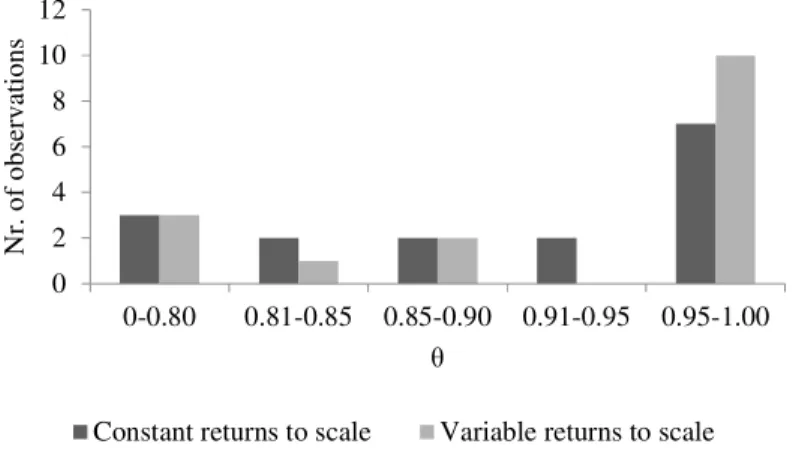
The figure below illustrates the efficiency scores distribution comparison between constant and variable returns to scale approach.

12_{For example, this is the case of Casu and Molyneux (2003).} 13_{The adaptation of C.C.R. Model allowing variable returns to scale.}

(37)

24 Figure 4: Efficiency scores distribution

Source: Author (2018).

In the case of constant returns to scale, four D.M.U.’s are considered to be efficient in the allocation of inputs (interest expense and deposits) to generate output (interest income and loans). However, for variable returns to scale, half of the sample is considered to be efficient in output generation. It should be observed that for both constant and variable returns to scale there are scores of 1.000 assigned to D.M.U.’s that are not in the first place in the ranking due to rounding. Within D.M.U.’s with an efficiency score of 1.00014

it is impossible to make any further distinction (Yeah, 2017).

Slack analysis

One of the major advantages of Data Envelopment Analysis is the high degree of precision when identifying inefficiency in the model applications. That is, when an inefficient D.M.U. is detected, it is possible to determine the ideal amount of output for that given input, and vice-versa. This constitutes a major advantage in the formal quantitative assessment of the efficiency performance in the German banking industry for the reference period under scrutiny.

Table 4 describes the slacks for the reference period 2016, considering constant returns to scale15_.

14_{To be more specific, to a D.M.U. to be considered efficient it is not only necessary to have an efficiency}

score of 1 but also to have a rank of 1 when comparing with the other DMUs.

15_{For simplification, the slacks for the variable returns to scale approach can be found in the Appendix.}

The rationale for the interpretation is the same as in the constant returns to scale approach. 0 2 4 6 8 10 12 0-0.80 0.81-0.85 0.85-0.90 0.91-0.95 0.95-1.00 N r. o f ob se rv at io ns θ

(38)

25

Table 4- Slack analysis for 2016 (constant returns to scale approach assumed)

DMU Output slack Input slack

Interest income Loans Interest expense Deposits

A . 180,000,000 . 0 B 0 . . 0 C 650,209 . . 0 D . 31,900,000 . 0 E . 3,101,785 . 2 F . 0 0 . G 1,298,784 4 659,780 . H . 5 776,668 . I 1,391,426 4 8,525 . J . 0 . 0 K 194,816 . . 0 L . 2,591,609 . 0 M . 4 909,001 . N 0 0 0 . O 41,388 . . . P 0 . . .

Slacks refer to additional improvements that might be implemented in order for a given D.M.U. to be fully efficient. Accordingly, input slack thus constitutes the input amount that could be reduced to efficiently produce that specific level of output. Similarly, output slack accounts for the increase in output necessary to achieve the efficient line for a given amount of input.

In order to better illustrate the model application, two examples are addressed. First, in Table 3, D.M.U. A has a theta of 0.931, taking into account that the application is conducted under the output-oriented approach. In this specific case, D.M.U. A could increase its output by 6.69% without affecting any variable. However, the said D.M.U. A can also increase the output loans by €180,000,000, even after increasing all outputs by 6.69%. A second example is related to D.M.U. G. In this case, the unit possesses an efficiency score of 0.885, which reflects the fact that, even after the increase of 11.5% of output, it could still increase interest income by €1,298,784k and decrease interest expense by €659,780k.

(39)

26

5.1.1. b) The One-input (deposits) and One-output (loans) Model Application

Input and output variable choice is extremely important for the model, insofar as the results of the model applications are sensitive to the number of chosen variables, both in terms of efficiency scores and ranking. In order to evaluate that effect in the present sample, and also to perform a partial variable analysis, the present research strategy contemplated two further levels of analysis: i) the deposits-loans model; and the ii) interest expense-interest income model.

Table 5 summarises the deposits-to-loans D.E.A. model, considering both constant and variable returns to scale.

Table 5 – D.E.A. model for deposits-to-loans approach (constant and variable returns to scale).

rank θ rank θ A 15 0.567 15 0.691 B 7 0.817 1 1.000 C 14 0.601 13 0.708 D 13 0.607 12 0.720 E 12 0.645 11 0.735 F 8 0.771 7 0.849 G 5 0.885 5 0.992 H 4 0.899 6 0.975 I 3 0.941 1 1.000 J 10 0.727 10 0.813 K 9 0.760 8 0.840 L 16 0.379 16 0.388 M 2 0.973 1 1.000 N 1 1.000 1 1.000 O 11 0.673 14 0.696 P 6 0.824 9 0.836 Min. 0.379 0.388 Median 0.766 0.838 Average 0.754 0.828 Std. dev. 0.169 0.170

The most efficient bank in the allocation of deposits and loans is bank N. Considering also the variable returns to scale scenario, the number of efficient D.M.U.s increases to four. D.M.U. N, which was the most efficient unit in the base case scenario, is still the

(40)

27

most efficient in this specific model application. The same observation could be stated regarding D.M.U. L, insofar as the least efficient unit in the base model still continues to be the least efficient unit under this specific framework analysis.

It should be mentioned that the average, minimum, and median values are consistently lower in this approach than in the above-mentioned base case, meaning that the average percentage potential improvement is higher than was the case with the base model.

5.1.1. c) The One-input (interest expense) and One-output (interest income) Model Application

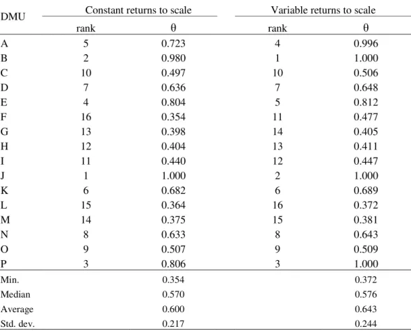
Table 6 presents a summary of the interest expense-interest income D.E.A. model application, considering both constant and variable returns to scale.

Table 6 – D.E.A. model for the interest paid to interest received approach (constant and variable returns to scale)

rank θ _rank θ A 5 0.723 4 0.996 B 2 0.980 1 1.000 C 10 0.497 10 0.506 D 7 0.636 7 0.648 E 4 0.804 5 0.812 F 16 0.354 11 0.477 G 13 0.398 14 0.405 H 12 0.404 13 0.411 I 11 0.440 12 0.447 J 1 1.000 2 1.000 K 6 0.682 6 0.689 L 15 0.364 16 0.372 M 14 0.375 15 0.381 N 8 0.633 8 0.643 O 9 0.507 9 0.509 P 3 0.806 3 1.000 Min. 0.354 0.372 Median 0.570 0.576 Average 0.600 0.643 Std. dev. 0.217 0.244

It can be observed that, in the case of constant returns to scale, just one D.M.U. (J) has an efficiency score of 1.000; whilst in the scenario of variable returns to scale, there are three

(41)

28 D.M.U.’s that achieve the perfect score (B, J and P), notwithstanding the fact that only D.M.U. B is located in the efficient frontier, since it not only has a score of 1.000 but also its rank equals 1.

Furthermore, it is also interesting to verify that D.M.U. J was the first in the ranking under C.R.S., but when applying V.R.S., it drops to the second place. On the other hand, D.M.U B is the second in ranking for C.R.S., but the first in V.R.S.

The most revenue efficient bank in Germany for this reference period is D.M.U. J (for constant returns to scale) and D.M.U. B (for variable returns to scale).

When comparing these findings with the one-input and one-output (deposits-loans) and with the two-input and two-output approach, we observe lower minimum, median and average values.

Furthermore, and when a comparison between the deposits-loans and interest paid-interest-received is addressed, the most efficient bank for the reference period is not the same. So, it is reasonable to state that, for this specific sample, efficiency is variable-sensitive.

5.1.2. Multi-year analysis (2013-2016)

5.1.2. a) Two-input and Two-output Model Application

The present section’s main line of argumentation is twofold: i) it first presents static efficiency scores relative to 2016); ii) it subsequently extends this line of argumentation by presenting dynamic efficiency scores in the context of more than just one single period. The present Dissertation’s line of argumentation is thus made more robust with this twofold approach.

Table 7 presents the output of D.E.A. estimation associated with the case of two inputs (interest expense and deposits) and two outputs (interest income and loans conceived). It is important to observe that constant returns to scale were used in this case16_.

(42)

29

Table 7 – Two-input and Two-output model for 2013-2016.

DMU 2013 2014 2015 2016 Average _rank

rank θ rank θ rank θ rank θ

A 5 0.986 8 0.942 7 0.975 9 0.931 7 B 1 _1.000 1 1.000 1 1.000 1 1.000 1 C 13 _0.802 10 0.885 11 0.888 15 0.691 12 D 14 _0.790 13 0.838 14 0.806 13 0.809 14 E 9 _0.889 7 0.960 6 0.979 12 0.819 9 F 4 _1.000 5 1.000 1 1.000 1 1.000 3 G 15 _0.729 15 0.766 16 0.765 10 0.885 14 H 11 _0.864 11 0.884 9 0.909 7 0.952 10 I 10 _0.888 14 0.811 15 0.775 8 0.941 12 J 1 _1.000 4 1.000 1 1.000 1 1.000 2 K 12 _0.811 9 0.895 12 0.878 11 0.884 11 L 16 _0.655 16 0.679 13 0.808 16 0.490 15 M 7 _0.897 12 0.859 10 0.895 6 0.991 9 N 1 _1.000 1 1.000 5 1.000 1 1.000 2 O 6 _0.985 1 1.000 8 0.965 14 0.752 7 P 8 0.890 6 0.992 1 1.000 5 1.000 5 Min _0.655 0.679 0.765 0.490 Median _0.890 0.919 0.937 0.936 Average 0.887 0.907 0.915 0.884 Std. dev. 0.107 0.098 0.087 0.143 Source of underlying data: ORBIS® BankFocus.

The above-mentioned dynamic findings prompt the following conclusions. First, the presented scores are typically high, with a minimum score associated with the 4-year window being 0.490 (D.M.U. L for 2016). Second, it is interesting to observe the persistency of ranking positions across the periods, especially for the first place, as bank B is always a reference for all the remaining German banks in all periods (from 2013 to 2016). Third, bank L ranks last for all years, with the exception of 2015. A tentative explanation for this fact will be detailed subsequently.

5.1.2. b) One-input (deposits) and One-output (loans)

Table 8 presents the One-input (deposits) and One-output (loans) model application for the 2013 – 2016 extended period (dynamic framework).