Constitutive modeling and mechanical behavior prediction of biodegradable polymers during degradation

Vieira, A.C., Guedes, R.M., Tita, V., “Constitutive modeling and mechanical behavior prediction of biodegradable polymers during degradation.” In: “Biodegradable Polymers. Volume 1: Advancement in Biodegradation Study and Applications”, Nova Publisher, 2015, p.31-75, ISBN 978-1-63483-632-6

Chapter

C

ONSTITUTIVE MODELING AND MECHANICAL

BEHAVIOR PREDICTION OF BIODEGRADABLE

POLYMERS DURING DEGRADATION

André C. Vieira

1

, Rui M. Guedes

2,3

, Volnei Tita

1

1

Aeronautical Engineering Department, São Carlos School of Engineering, University of São Paulo, São Carlos, São Paulo, Brazil

2

Mechanical Engineering Department, Faculty of Engineering of University of Porto, Porto, Portugal

3

Porto Biomechanics Laboratory, University of Porto, , Porto, Portugal

A

BSTRACT

A large range of biodegradable polymers has been used to produce implantable medical devices, such as suture fibers, fixation screws and soft tissue engineering devices. Apart from biological compatibility, these devices should also be functional compatible and perform adequate mechanical temporary support during the healing process. The mechanical behavior of biodegradable polymers is known to be rate dependent and to exhibit hysteresis upon cyclic loading. On the other hand, ductility, toughness and strength of the material decay during hydrolytic degradation. Continuum based mechanical models can be used as dimensioning tools for biodegradable polymeric devices, since they enable to predict its mechanical behavior in a complex load and environment scenario, during the hydrolytic degradation process.

The existing models can be divided into two categories: the time-dependent models and the time-independent models. Linear elastic or non-linear elastic models, such as elasto-plastic or hyperelastic models, can simulate the time-independent response, which corresponds to the relaxed configuration and represent the relaxed state. However, these approaches neglect the time-dependent mechanical behavior. To consider time dependency, dissipative elements must be used in the model formulation.

A revision of the three-dimensional constitutive models generally used for polymers is presented in this chapter. These models are based on the concept of networks, combining elastic, sliding and dissipative elements, in order to simulate the time-dependent mechanical behavior, although neglecting changes in the properties of the material during hydrolytic degradation process. Thus, some of these models were recently adapted to address the hydrolytic degradation process. A common method consists on becoming some of the material model parameters dependent on a scalar variable, which expresses the hydrolytic damage.Furthermore, the advantages and limitations of the models are discussed, based on the correlation between predictions and experimental results of a blend of polylactic acid and polycaprolactone (PLA-PCL), which include monotonic tensile tests at different strain rates and quasi-static cyclic unloading-reloading.

Keywords: constitutive models, mechanical behavior, biodegradable polymers, hydrolytic degradation

I

NTRODUCTION

Biodegradable polymers can be classified as either naturally derived polymers or synthetic polymers. A large range of mechanical properties and degradation rates are possible among these polymers. However, the prediction of the mechanical behavior of these biodegradable devices is complex, because not only the mechanical properties evolve during degradation, but also these biodegradable polymers, in many situations, cannot be modeled using simple elastic constitutive equations. Due to the nonlinear nature of the stress vs. strain relation, the classical linear elastic model is not valid for simulation under large strains. Current designs of biodegradable devices are carried out by considering elastic or elastoplastic behavior and neglect any changing on the mechanical behavior of the device with degradation (Moore et al., 2010). For many biomedical applications, the biodegradable polymeric structures are submitted to cyclic loading above the elastic limit. Hence, they are prone to accumulate plastic strain at each cycle, which may lead to laxity and consequent failure. For instance, Grabow et al. (2007) showed that significant creep of polylactides under a constant load leads to strain accumulation and collapse.

Concomitantly to its nonlinear nature, the mechanical behavior of polymeric materials is also temperature and strain rate dependent (Bardenhagen et al., 1997). However, due to isothermal host environment, when the implantable devices are in service, temperature dependence will be neglected in this chapter. Moreover, under low strain rates, the mechanical behavior is viscous and, under high strain rates, it becomes brittle elastic (Bardenhagen et al., 1997). Thus, the polymeric mechanical behavior should be modeled by different constitutive laws, considering the strain rate range of interest (Ferry, 1980, Ward, 1979). For example, Soares (2008) and Grabow et al. (2007) confirmed the non linear viscoelastic characteristics of PLA. The mechanical behavior of biodegradable polymers is also known to exhibit hysteresis, i.e. energy dissipation in form of heat upon cyclic loading, as shown by Vieira et al. (2013) for PLA-PCL. Therefore, time-dependent constitutive models are required to simulate such phenomena.

As observed in polymers, it is known that the stress in a biodegradable polymer will relax towards an equilibrium state after being subjected to a strain-step (Miller and Williams, 1984). This relaxed state has been simulated by linear elastic, elasto-plastic or hyperelastic models, but disregarding the rate dependency effect. Moreover, the response of an elastic or hyperelastic material model implies that the loading and unloading paths coincide. Mechanical properties of biodegradable polymers are commonly assessed within the scope of linearized elasticity, despite the large strains, which are observed before material fracture. Thus, inelastic or hyperelastic models are required to simulate such strain range. Hence, considering the response of biodegradable polymers, classical models such as the neo-Hookean and Mooney-Rivlin models, usually applied for incompressible hyperelastic materials, have been used to predict mechanical behavior until rupture of non-degraded PLA (Garlotta, 2001, Lunt, 1998) under quasi-static monotonic loading. A single-order, isotropic Ogden material hyperelastic model was also used (Krynauw et al., 2011) to simulate the mechanical behavior evolution during degradation of a polyester-urethane scaffold. However, those approaches neglect changes in the properties of the material during degradation process.

In the case of elasto-plastic models, after unloading phase, the material returns to a relaxed equilibrium sate, which includes inelastic strain. Since these models include at least one sliding element in its formulation, the loading and unloading paths do not coincide. Although, those models neglect the time-dependent mechanical behavior, they can simulate the time-independent response, which corresponds to the relaxed configuration.

To consider time dependency, dissipative elements represented by time inhomogeneous relations must be used in the model formulation. The simplest viscoelastic models consider a linear combination of springs (using the Hooke’s law) and dashpots (using Newtonian damper with linear viscosity). More complex variants of these simple models are based on the same concept of networks, combining elastic, sliding and dissipative elements, in order to simulate the equilibrium response of the material and the time-dependent deviation from equilibrium relaxed configuration.

However, those models are only able to simulate the initial mechanical behavior of polymers, neglecting changes in the properties of the material during the hydrolytic degradation process. It is possible to find only few scientific contributions in the literature (Khan and El-Sayed, 2013, Muliana and Rajagopal, 2012, Soares, 2008; Soares et al., 2010, Vieira et al. 2014) about the simulation of the mechanical behavior of biodegradable polymer during the hydrolytic degradation process. Therefore, the aim of this chapter is to explain a methodology to adapt different constitutive models in order to simulate the mechanical behavior during the hydrolytic degradation process. The concept behind this type of approach is to change the material model parameters as function of a scalar field, which represents the hydrolytic degradation and the correspondent chemical damage, inducing the changes of the mechanical behavior of the biodegradable materials. Hence, in the next section, there is a presentation about biodegradation process, namely describing the physical-chemical mechanisms and a simple way to model the degradation process based on the random scission assumption. Furthermore, the hydrolytic damage is defined and a failure criterion is established for biodegradable materials as function of degradation time. Then, after that, there is a brief review of some constitutive models generally used to simulate the mechanical behavior of conventional polymers under hydrolytic degradation by using the proposed methodology. Some examples are shown, and the potential of each type of constitutive model are discussed and compared for different loading situations.

B

IODEGRADATION PROCESS

All biodegradable polymers contain hydrolysable or oxydable bonds. This makes the material sensitive to moisture, heat, light and also mechanical stress. These different types of polymer degradation (photo, thermal, mechanical and chemical degradation) can be present alone or combined, working synergistically to the degradation. Usually, the most important degradation mechanism of biodegradable polymers is chemical degradation via hydrolysis or enzyme-catalyzed hydrolysis (Göpferich, 1996). Hydrolysis rate is affected by the temperature or mechanical stress, molecular structure, ester group density as well as by the degradation media used. The crystalline degree may be a crucial factor, since enzymes attack mainly the amorphous domains of a polymer. The most important factor is its chemical structure and the occurrence of specific bonds along its chains. Like those in groups of esters, amides, etc., which might be susceptible to hydrolysis when exposed to water (Nikolic et al., 2003; Herzog et al., 2006).

Another important distinction must be made between erosion and degradation. Both are irreversible processes. The erosion process can be described by phenomenological diffusion-reaction mechanisms. An aqueous media diffuses into the polymeric material while oligomeric products diffuse outwards to be then bio-assimilated by the host environment. Then, there is material erosion with correspondent mass loss. Hence, the degree of erosion is estimated from the mass loss. On the other hand, degradation refers to mechanical damage and depends on hydrolysis. Within the polymeric matrix, hydrolytic reactions take place, mediated by water and/or enzymes. Polymer degradation is the first step of the erosion phenomenon and can be estimated by measuring the evolution of molecular weight, by size exclusion chromatography (SEC) or gel permeation chromatography (GPC), or the tensile strength evolution (by universal tensile testing). Therefore, the hydrolytic degradation process is included on the erosion process. The complete erosion of the polymer is known to take substantially longer than the complete loss of tensile strength. During this first phase, aqueous solution penetrates the polymer, followed by hydrolytic degradation, converting these very long polymer chains into shorter water-soluble fragments.

Physical-Chemical mechanisms and modeling

Hydrolysis has been traditionally modeled by using a first order kinetics equation based on the random scission kinetic mechanism of hydrolysis, according to the Michaelis–Menten scheme (Bellenger et al., 1995). In the case of aliphatic polyesters, such as PLA, each polymer molecule, with its own carboxylic and alcohol end groups, is broken in two. This occurs randomly in the middle at a given ester group. So, the number of carboxylic end groups will increase with degradation time, while the molecules are being split by hydrolysis. The following first-order equation describes the hydrolytic process (Farrar and Gilson, 2002), in terms of the rate of formation of carboxyl end groups:

uc

kewc

dt

dc

₌

₌

Eq. 1

where e, c and w are the concentrations of ester groups, carboxyl groups and water in the polymer, respectively. k is the hydrolysis rate constant and t is the degradation time. u is the hydrolytic degradation rate of the material, which can be determined by measuring strength or molecular weight evolution during hydrolytic degradation (see Vieira et al., 2011a). Since the concentration of carboxyl end groups is given by c=1/Mn, where Mn is the number-average

molecular weight of the polymer, the evolution of the number-average molecular weight is given, after integration, by:

ut n n

M

e

M

0 t −

=

Eq. 2

where Mnt is the number-average molecular weight of the polymer at degradation time t

and Mn0 is the initial (non-degraded) value. Degradation rate u is affected by many factors

that can vary along the volume or during degradation. For example, temperature will increase the hydrolysis rate constant k, which is associated to the probability of bond scissions, due to excitement of the molecules. In the case of implantable devices, the temperature is kept constant as in the human body, i.e. at the homeostatic value around 37ºC.

The influence of the mechanical environment in the degradation rate has been also reported at literature (Chu, 1985; Miller and William, 1984). Similarly to temperature, stress applied during the degradation process also increases the probability of bond scissions, and

consequently increases the degradation reaction rate constant k. Some studies on rubbery polymers include the effect of micro structural changes in the polymer’s macromolecules, crosslinks and entanglements (Huntley et al., 1996; Rajagopal et al., 2007; Rajagopal and Wineman, 1992; Shaw et al., 2005; Smeulders and Govindjee, 1999; Wineman and Min, 2002). In those approaches, not specifically related to hydrolytic degradation, micro structural changes depend on state variables, which locally measure chain stretches. Later, other researchers (Khan and El-Sayed, 2013; Muliana and Rajagopal; 2012, Soares, 2008; Soares et al., 2010) developed their methodologies based on those works previously published, in order to introduce the influence of the strain field in the hydrolytic degradation.

Concerning the degradation dependence, some authors reported that the degradation rate of PLA and blends of PLA-PCL was significantly affected by some enzymes (Gan et al., 1999; Williams, 1981). The pH of the aqueous media also affects the degradation reaction rate constant k (Tsuji and Ikada, 1998; Tsuji and Ikada, 2000; Tsuji and Nakahara, 2001). Again, in the case of implantable device, pH can be considered constant, because, pH is kept at a homeostatic value in the human body. Hence, in many cases, it can be assumed that the hydrolysis rate k is constant over time due to constant temperature, load (i.e. constant stress field during degradation) and degradation media.

In the particular case of biodegradable polymers, water diffusion is very fast compared to water-mediated hydrolysis. Therefore, water can be assumed, in many cases, to be spread out uniformly in the sample volume (i.e. no diffusion control) from the beginning of erosion process, and hydrolysis promotes homogeneous bulk erosion (Li et al., 1990). This assumption is reasonable for small thickness or porous devices.Hence, w can also be assumed constant from the beginning along the volume. Otherwise, the water concentration along the volume and during time can be computed using the Fick’s Second Law. In this early stage of erosion, when mechanical strength reduces significantly, the concentration of ester groups e located at the backbone chains is nearly constant. Despite of the scissions, which occur randomly in the ester groups, the macromolecules remain large (Göpferich and Langer, 1993). Considering all this assumptions, the degradation rate, u=kwe, may be considered constant during the whole degradation process. In some cases, as explained previously, these assumptions are not valid, mainly because of heterogeneous diffusion of water, or due to the presence of a complex three-dimensional stress field, which evolves during the degradation process.

Hydrolytic damage and failure criteria

It is well known that the mechanical behavior will evolve during time, due to hydrolytic chain scission in the polymeric macromolecules. In figure 1a is shown the mechanical response to uniaxial monotonic tensile tests until rupture for PLA-PCL fibers during hydrolytic degradation The reduction of molecular weight is linked to this evolution in mechanical response of biodegradable polymers. It has been shown by Vieira et al. (2011a) that the fracture strength σduring degradation can be predicted by the following equation:

kwet 0 ut 0 t

e

e

− −

₌

=

σ

σ

σ

Eq. 3

where σt is the strength of the polymer at degradation time t and σ0 is the initial

(non-degraded) strength. The evolution of fracture strength, according to equation 3, is similar to the evolution of the number-average molecular weight of the polymer (see figure 1b) in accordance to equation 2. In a semi logarithmic representation of normalized strength or number-average molecular weight versus degradation time, the degradation rate u

corresponds to the slope of the linear fit. Further details of this degradation study can be found in Vieira et al. (2011a).

Figure 1 – a) Monotonic tensile test results during hydrolytic degradation of PLA-PCL fibers; b) Evolution of the normalized strength and molecular weight during degradation of

PLA-PCL fibers (adapted from Vieira et al., 2011a)

The hydrolytic damage was defined by Vieira et al. (2011a), according to equation:

ut n n 0 t h

1

e

M

M

1

1

d

o t

=

−

−

−

=

−

=

σ

σ

Eq. 4

From equation 4, it is possible to relate hydrolytic damage with strength and molecular weight. Hence, hydrolytic damage is a local internal variable since the degradation rate can vary locally in the case of heterogeneous degradation. In order to simulate the evolution of the mechanical behavior of biodegradable polymers, the constitutive models must be adapted accordingly to hydrolytic damage dh.

It is possible to find only few scientific contributions in the literature about modeling of the mechanical behavior of biodegradable polymers during the hydrolytic degradation process. Those approaches are based on hyperelastic models (Soares et al., 2010; Vieira et al., 2011a), or on quasi-linear viscoelastic models (Muliana and Rajagopal, 2012), or on viscoplastic models (Khan and El-Sayed, 2012; Vieira et al., 2014). These approaches enable the modeling of biodegradable structures during degradation by assuming that the constitutive model parameters have been changed according to hydrolytic damage. In Muliana and Rajagopal (2012), hydrolytic damage is assumed to be dependent on the deviatoric strain tensor and the concentration of water.

C

ONSTITUTIVE MODELS

F

OR

P

OLYMERS WITH BIODEGRADATION PROCESS

Continuum mechanics is always the base for the generalization of constitutive models to three-dimensional approach. Hence, for the sake of completeness, there is a brief review and definitions on finite continuum mechanics in the Appendix and more details can be found in Malvern (1969). A constitutive model for a mechanical analysis is a relationship between the response of a body (for example, strain state) and the stress state due to the forces acting on the body, which can include the environmental effects. The actual models can be divided into two main categories: the time-independent and the time-dependent models.

Linear elastic constitutive model

In uniaxial models, the applied stress, considered uniform along the surface perpendicular to the applied load, is the ratio between the applied load and the initial surface area (nominal stress, i.e. Lagrange description), σ=F/A0, or alternatively the ratio between the applied load

and the current surface area (true stress, i.e. Euler description), σ=F/A. In this case, the linear strain is defined by the ratio between elongation and the initial length, ε=(L- L0)/L0, and

stretch is defined by the ratio between current length and the initial length, λ=1+ ε =L/L0. The

uniaxial linear elastic model (the Hooke’s law) establishes a linear relation between stress and strain, σ= Eε, defined by a single material parameter E (Young modulus). This linear elastic rheological model is represented by a linear spring.

The generalization of the linear constitutive model to three-dimensional approach, according to a Largrange description, considering relation between the second Piola-Kirchhoff stress tensor S and the Lagrangian strain tensor E (see definitions in Appendix), is defined by an elastic stiffness fourth order tensor C:

kl ijkl

ij

C

E

S

=

Eq. 5

Alternatively, in the Euler description, considering the relation between the Cauchy stress tensor T and the Eulerian strain tensor E* (see definitions in Appendix):

* kl * ijkl ij

C

E

T

=

Eq. 6

The relation between the two elastic stiffness tensors, in the Lagrange and Euler descriptions, is: nl mk pqkl jq ip nl mk pqkl jq ip * ijnm

J

1

R

R

C

R

R

F

F

C

F

F

C

=

≈

Eq. 7

where the Jacobian J, the deformation gradient F and the rotation tensor R are defined in Appendix.

Due to the isotropic nature of polymers, only isotropic models will be discussed in this chapter. Hence, considering an isotropic material, only two independent material parameters are needed to define all the components of the elastic stiffness fourth order tensor. Most commonly, the generic three-dimensional linear constitutive model, for isotropic materials, is presented in the form (according to Lagrange and Euler description respectively):













−

+

+

=

ij kk ij ij

2

1

1

E

δ

υ

υ

υ

E

E

S

Eq. 8













−

+

+

=

ij * kk * ij ij

2

1

1

E

_δ

υ

υ

υ

E

E

T

Eq. 9

where the Young’s modulus E and the Poisson’s ratio υ are the two independent material parameters. The Kronecker delta function δij is defined in Appendix. If the stress tensor is

known, it is possible to compute the strain tensor using the inverse relation:

kl ijkl ij

S

S

E

=

Eq. 10 kl * ijkl * ij

S

T

E

=

Eq. 11

where

S

_ijkl and

S

*_ijkl are elastic compliance fourth order tensors in the Lagrange and Euler descriptions, respectively. Therefore, for isotropic materials, the constitutive relation may have the form:

ij kk ij ij

E

E

1

υ

υ

_δ

S

S

E

=

+

−

Eq. 12

The fourth order stiffness and compliance tensors, for isotropic materials, are hence defined respectively:

(

)

(

)

(

)(

)

(

il jk ik jl

)

ij kl kl ij jl ik jk il ijkl

2

1

1

E

1

2

E

δ

λδ

δ

δ

δ

δ

µ

δ

δ

υ

υ

υ

δ

δ

δ

δ

υ

+

+

=

=

−

+

+

+

+

=

C

Eq. 13

(

il jk ik jl

)

ij kl ijkl

E

E

2

1

+

υ

_δ

_δ

₊

_δ

_δ

₋

υ

_δ

_δ

=

S

Eq. 14

where the shear modulus,

µ

=

E

/

2

(

1

+

υ

)

, and the Lamé’s constant,

λ

=

E

υ

/

(

1

+

υ

)(

1

−

2

υ

)

, are other alternative material parameters commonly used to characterize the elastic behavior of polymers. Another material parameter usually found in the Hooke’s generalized model is bulk modulus,

κ

=

E

/

3

(

1

−

2

υ

)

.

Linear elastic model is unable to capture yielding. Moreover, it is possible to see in figure 1a) that, in the linear region, the Young modulus E remains nearly unchanged during degradation. However, at large strains, the linear elastic model is able to fit reasonably well the experimental monotonic tensile test results. Another limitation of this model is that it is time-independent. Hence, it is unable to capture the mechanical behavior dependence on the strain rate, as can be seen in figure 2a for the monotonic tensile test at two different strain rates (15 and 500 mm/min), when both experimental results were used to calibrate the

parameters of the model by inverse analyses. It is also unable to capture hysteresis and plastic strain accumulation, since the unloading path is the same of the reloading path (see figure 2b). In this second case, unloading-reloading tensile tests results were used to calibrate the model parameters. On one hand, the linear elastic model predicts the same result independently from the strain rate (see figure 2a). On the other hand, the loading and unloading paths coincide in the same linear prediction. The calibration technique used to minimize the difference between the experimental results and the model predictions was the Nelder-Mead method.

Figure 2 –Experimental results of a) monotonic tensile test at two strain rates (500 and 15 mm/min) and b) cyclic tensile test of a biodegradable polymer (PLA-PCL), and prediction of

linear elastic model.

Calibration of the model was done based on the monotonic tensile tests results (at 250 mm/min) at four degradation steps (0, 2, 4 and 8 weeks). Considering that the Poisson’s ratio

υ remains unchanged (0.4) during degradation, the elastic modulus E was determined by

calibration at each degradation step. Then estimated values were fitted by linear regression as function of the degradation damage d(t,u). In the figure 3, it is possible to observe that the elastic modulus E decreases nearly linear as function of the hydrolytic damage.

E = -793.12dh+ 1489.4 R² = 0.9407 1000 1100 1200 1300 1400 1500 1600 0.0 0.1 0.2 0.3 0.4 0.5 0.6



dh Linear elastic

Figure 3 –Evolution of the elastic modulus E during hydrolytic degradation.

Based on this linear equation to estimate the elastic modulus E(d), the mechanical behavior of the polymer was predicted. The results are shown in figure 4.

Figure 4 – Experimental results of monotonic tensile test at 250 mm/min of PLA-PCL fiber, and model results via linear elastic model, after 0, 2, 4 and 8 weeks of hydrolytic degradation.

Hyperelastic constitutive models

Besides the linear elastic model, hyperelastic models can be used to model the relaxed state. Polymeric materials are known by their non-linear mechanical behavior. Hyperelastic models are a class of constitutive relationships able to model nonlinear elasticity. Mechanical properties of hyperelastic materials are usually represented in terms of a strain energy density function W. Considering the one-dimensional representation of hyperelastic models, the constitutive relation is generically defined by:

ε

σ

d

dW

=

Eq. 15

where σ and ε are the stress and strain measured by the uniaxial tensile test, where W is defined by:

( )

∫

=

σ

ε

d

ε

W

Eq. 16

and represents the area below the stress-strain curve. Hyperelastic models should have the ability to reproduce the ‘S’ shaped response of rubber like materials (Chagnon et al., 2004).

A general polynomial form usually found for the strain energy density, assuming an incompressible mechanical behavior, is defined in terms of the strain invariants:

( )

∑

(

) (

)

=

−

−

=

N 0 j , i j i ij

I

3

II

3

c

II

,

I

W

Eq. 17

where

I

=

λ

2

+

2

/

λ

is the first invariant and

II

=

1

/

λ

2

+

2

λ

is the second invariant and cij are material parameters.

In the case of hyperelastic models, generalizing to the three-dimensional representation,

W is a scalar function of the deformation gradient F. The rate of work done by stresses acting

on a small material element with volume dV0 in the undeformed solid may be defined as:

0 ij ij ij ij

dV

t

W

t

W

W

F

F

P

F

ɺ

ɺ

=

∂

∂

∂

∂

=

∂

∂

=

Eq. 18

Then, a generic form for a hyperelastic constitutive relation can be presented in terms of the first Piola-Kirchhoff stress tensor P:

ij ij

W

F

P

∂

∂

=

Eq. 19

or in terms of Cauchy stress tensor T:

kj ik ij

W

J

1

F

F

T

∂

∂

=

Eq. 20

As referred previously for the one-dimensional model, this constitutive relation is usually defined in terms of the invariants of the left Cauchy-Green deformation tensor B (see definition in Appendix). The first, second and third invariants are defined, respectively, as:

( )

2 3 2 2 2 1 kk ij B

tr

I

=

B

=

B

=

λ

+

λ

+

λ

Eq. 21

[

]

2 1 2 3 2 3 2 2 2 2 2 1 ki ik 2 B B

I

2

1

II

=

−

B

B

=

λ

λ

+

λ

λ

+

λ

λ

Eq. 22 2 3 2 2 2 1 2 kk B

J

III

=

B

=

=

λ

λ

λ

Eq. 23

where , = 1, 2, 3 are the eigenvalues of F, and also known as principal stretches. The formulas for the strain energy function are generally expressed in terms of principal stretches:

(

)

∑

{

[

(

) (

) (

)

]

(

)

}

=

−

+

+

+

+

+

=

N 0 k , j , i k 3 2 1 j 2 j 1 i 3 j 1 j 3 i 2 j 3 j 2 i 1 ijk 3 , 2 , 1

a

6

W

λ

λ

λ

λ

λ

λ

λ

λ

λ

λ

λ

λ

λ

λ

λ

Eq. 24

where

a

_ijk are material parameters, or in terms of the invariants of the Cauchy-Green deformation tensors:

(

)

∑

(

) (

) (

)

=

−

−

−

=

N 0 k , j , i k B j B i B ijk B B B

,

II

,

III

c

I

3

II

3

III

3

I

W

Eq. 25

where

c

_ijk are material parameters. Many elastomeric and polymeric materials are often nearly incompressible. Hence, it is more convenient to use an alternative set of invariants of the deviatoric left Cauchy-Green tensor (i.e. neglecting the volumetric part of the strain tensor): B 3 / 2 B

J

I

I

=

− Eq. 26 B 3 / 4 B

J

II

II

=

− Eq. 27

Therefore, it is common to find the strain energy density function in the generic polynomial form (Forni et al., 1999), in terms of this alternative set of invariants:

(

)

∑

(

) (

)

∑

(

)

=

−

+

−

−

=

N 0 k , j , i M i i 2 i j B i B ij B B

,

II

,

J

c

I

3

II

3

d

J

1

I

W

Eq. 28

where cij are the material parameters related to distortion, whereas di are the material

parameters related to volume change. Note that for incompressible materials J is equal to “1”. Particular cases of this general polynomial form, considering

W

(

I

B

,

II

B

,

J

)

, are: - the Neo-Hookean model, where i=1, j=0 and N=M=1:

(

) (

)

(

)

2 1 B 10 B B

,

II

,

J

c

I

3

d

J

1

I

W

=

−

+

−

Eq. 29

Solving equation 20, the corresponding constitutive relation results in:

(

)

ij 1 ij kk ij 3 / 5 10 ij

2

d

J

1

3

1

J

c

2

δ

δ



+

−











−

=

B

B

T

Eq. 30

- the Mooney-Rivlin model, where c00=0, c11=0, and N=1:

(

) (

) (

)

(

)

2 1 B 01 B 10 B B

,

II

,

J

c

I

3

c

II

3

d

J

1

I

W

=

−

+

−

+

−

Eq. 31

[ ]

ij ik ki kn nk ij 1

(

)

ij 2 kk ij kk 3 / 7 01 ij kk ij 3 / 5 10 ij

1

J

d

2

3

1

3

1

J

c

2

3

1

J

c

2

δ

δ

δ

δ

−

+













+

−

−

+

+













−

=

B

B

B

B

B

B

B

B

B

T

Eq. 32

where in these cases 2d1=κ. The simplest hyperelastic model for elastomeric materials is

the Neo-Hookean model. It is a Gaussian statistical theory model, because the strain energy function was originally defined as:

(

)

(

3

)

2

T

n

3

I

2

W

23 2 2 2 1 B

−

=

+

+

−

=

µ

β

λ

λ

λ

Eq. 33

where the shear modulus µ is a function of the chain density (n), Boltzmann’s constant (β) and temperature (T). See Treloar (1975) for a more detailed description of Gaussian statistics and the corresponding assumptions. On the other hand, the Mooney-Rivlin model is an empirical model. Although it is one of the most favorite models, its disadvantage is that material parameters must be obtained by mechanical experiments since they are not physically consistent. Other sophisticated empirical models, variants of the generic polynomial forms, such as Odgen model or Yeoh model, can be found in literature.

A good constitutive model should represent the three-dimensional nature of the stress-stretch behavior using a minimal number of parameters to represent physically the deformation process. Ideally, the parameters should be obtainable from a small number of experiments, preferably only one (Arruda and Boyce, 1993b). In this sense, Yeoh model is an empirical simple model, applicable for a wider range of deformation and is able to predict the stress-strain behavior in different deformation modes (such as compression or shear) from data gained in one simple deformation mode (such as uniaxial extension)(Ghosh et al., 2003). Other physical models are based on chains networks described by Gaussian statistics or modified by the chain statistics to allow larger stretches than those afforded by the Gaussian statistics assumption. They incorporated these non-Gaussian chains into networks of three, four or an infinite number of chains (Wang and Guth, 1952; Flory and Rehner, 1943; Treloar, 1946). These models have in common two physically based parameters, the shear modulus (µ) and a chain locking stretch (λL) defined as the value of the chain stretch when the chain

length reaches its fully extended state. However, these refereed models fail in the task of describing the response of an elastomeric material under different states of deformation without changing the model parameters (Arruda and Boyce, 1993b). The Arruda-Boyce model, also known as eight-chain model, is a sophisticated physical model able to predict the stress-strain behavior in different deformation modes from data gained in one simple deformation mode. It can be considered an extension of the Neo-Hookean model, which considers non-linear Langevin chain statistics when deriving the strain energy function. The strain energy is assumed equal to the sum of the strain energies of the individual chains randomly oriented in space, as defined below (Raoult et al., 2005):

(

)

(

)

(

)

( )

(

)

(

)

2 1 3 B L 2 B L B N 1 i 2 1 i i B 2 i 2 L i

1

J

d

...

27

I

1050

11

9

I

20

1

3

I

2

1

1

J

d

3

I

c

W

−

+













+

−

+

−

+

−

=

=

−

+

−

=

∑

= −

λ

λ

µ

λ

µ

Eq. 34

with the first five terms ci for the Taylor expansion of an inverse Langevin function are

c1=1/2, c2=1/20, c3=11/1050, c4=19/7000, c5=519/673750. The corresponding constitutive

relation is:

(

)

ij 1 ij kk ij 4 L 3 / 4 kk 2 L 3 / 2 kk 3 / 5 ij

2

d

J

1

3

1

...

J

525

33

J

5

1

J

λ

λ

δ

δ

µ

_

₊

₋











−













+

+

+

=

B

B

B

B

T

Eq. 35

Although, hyperelastic models are non-linear they are unable to capture yielding. However, at large strains, they are able to fit reasonably well the experimental monotonic tensile test results. Another limitation of these types of models is that they are not time-dependent. Hence, similarly to the linear elastic model, they are unable to simulate the mechanical behavior dependence on the strain rate, as can be seen in figure 5a for the monotonic tensile test at two different strain rates (15 and 500 mm/min), when both experimental results were used to calibrate the parameters of the model by inverse analyses. They are also unable to capture hysteresis and plastic strain accumulation, since the unloading path is the same of the reloading path (see figure 5b). In this second case, unloading-reloading tensile test results were used to calibrate the model parameters. The same calibration technique was used.

Figure 5 –Experimental results of a) monotonic tensile test at two strain rates (500 and 15 mm/min) and b) cyclic tensile test of a biodegradable polymer (PLA-PCL), and prediction via

Arruda-Boyce model.

Calibration of the Arruda-Boyce model was done based on the monotonic tensile tests results (at 250 mm/min) at four degradation steps (0, 2, 4 and 8 weeks). Considering that the

material is nearly incompressible, therefore the bulk modulus κ is constantly high (40000 MPa), and the locking stretch λL also remains constant, since the predicted results are almost

insensitive for values close to 10. The shear modulus µ was determined by calibration at each degradation step. Then, estimated values were fitted by linear regression as function of the degradation damage d(t,u). In the figure 6, it is possible to observe that the shear modulus µ decreases nearly linear as function of the hydrolytic damage.

= -199.08dh+ 422.84 R² = 0.868 300.00 350.00 400.00 450.00 0.0 0.1 0.2 0.3 0.4 0.5 0.6



dh Arruda-Boyce

Figure 6 –Evolution of the shear modulus µ during hydrolytic degradation.

Based on the linear equation to estimate the elastic modulus µ (d), the mechanical behavior of the polymer was predicted. The results are shown in figure 7.

Figure 7 – Experimental results of monotonic tensile test at 250 mm/min of PLA-PCL fiber, and model results via Arruda-Boyce model, after 0, 2, 4 and 8 weeks of hydrolytic

degradation.

These previous examples using the linear elastic and the hyperelastic Arruda-Boyce models enable the modeling of biodegradable structures during degradation. These methods to predict the mechanical behavior during degradation are based on the same concept developed in recent works (Soares, 2010; Vieira et al., 2011a) by assuming that the

constitutive model parameters have been changed according to hydrolytic damage. In these works other hyperelastic constitutive models, such as Neo-Hookean and Mooney-Rivlin, are used.

In another work (Vieira et al., 2011b), the Neo-Hookean hyperelastic model was implemented in ABAQUS through a User Material (UMAT) subroutine and PYTHON language. This script is run by ABAQUS and the degradation time is required as an input parameter data. The hydrolysis rate of the material u and the strength of the non-degraded material σ0 are initially set. Then the script calculates the hydrolytic damage dh according to

equation 4 and the material strength σt, according to equation 3, was used in an implemented

failure criterion in order to simulate a PLA-PCL fiber mechanical behavior until rupture in different stages of degradation, where is given the degradation time t. The script also calculates the material parameter c10 as a linear function of the hydrolytic damage dh. In

Vieira et al. (2011b), the load, or the stress field, was assumed constant during hydrolytic degradation, since the specimens degraded in a stress free state.

In the work of Soares et al. (2010), the rate of degradation depends on the deformation gradient d(F) and implicitly on both location and time. They defined the deformation-dependent reaction rate using the first and second invariants of the left Cauchy tensor,

B

_ij, that is:

(

)(

[

) (

₂

)

₂

]

2

3

3

1

1

₋

₋

₋

=

∂

∂

B B d h

II

I

d

t

d

τ

Eq. 36

where

τ

_d is the characteristic time of degradation. As consequence, inhomogeneous deformations, occurring in the body, can cause that some parts of it to degrade faster than others. However, these hyperelastic models neglect the time-dependent mechanical behavior. As seen before, they are unable to predict relaxation and creep.

Elastoplastic constitutive models

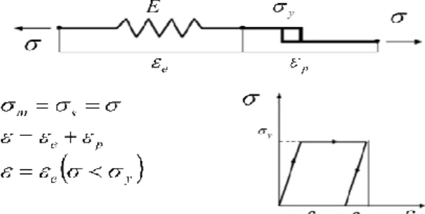
Elastoplastic models are commonly used to simulate the mechanical behavior of metals, including the yielding and hardening phenomena. In certain conditions, some features of the mechanical behavior of polymers can also be simulated using these types of models. One of the classical models described in literature is Saint-Venant plastic model, which represents a solid sliding over a surface with some friction (see figure 8). The yield stress is a material parameter, which represents the value above yielding, otherwise if this value is below, then there is no strain.

Figure 8 - Rheological representation of the perfectly plastic model

According to the Boltzmann superposition principle, elastic and sliding elements can be combined in series or in parallel. Regarding this principle, each loading step produces independent contribution to total loading history and the total final deformation is the sum of each contribution. Thus, it is possible to model the elastic perfectly plastic model (Prandlt-Reuss model), represented in figure 9, where the elastic and sliding elements are combined in series.

Figure 9 - Rheological representation of the elastic perfectly plastic model

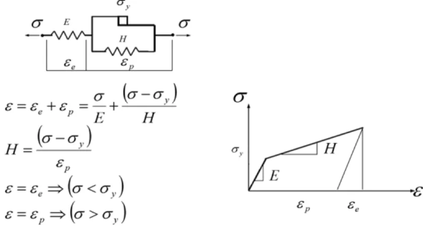
It is also possible to combine elastic and sliding elements in parallel (see figure 10), adding the linear isotropic hardening into the perfectly plastic model. The material parameter

H represents the hardening rate.

Figure 10 - Rheological representation of the linear isotropic plastic model

Another classical example of a plastic model is the power law isotropic hardening, represented in figure 11.

Figure 11- Rheological representation of the power law isotropic plastic model To model the elastoplastic mechanical behavior of polymer and the permanent plastic strain εp accumulated after a load cycle, the bilinear elastoplastic model represented in figure

12 is also widely used. It results from the combination in series of linear isotropic plastic model and a linear elastic model.

Figure 12- Rheological representation of the bilinear isotropic elastoplastic model In these one-dimensional models, total strain can be decomposed in an elastic part, recovered when the material is unloaded, and a plastic irreversible part, which remains after unloading:

p

e

ε

ε

ε

=

+

Eq. 37

For the generalization of this decomposition, in the case of three-dimensional constitutive elastoplastic models, the general strain increment is considered. According to a Lagrange description, this decomposition is defined as:

p ij e ij ij

d

d

d

E

=

E

+

E

Eq. 38

The linear constitutive relation for the elastic parcel results:

kl ijkl

ij

d

d

S

=

C

E

Eq. 39

A yield criterion must be established for the plastic part, to determine the critical stress state required to cause permanent deformations in the polymer. The two most used criteria are the von-Mises and the Tresca, defined respectively by their yield surface:

(

)

[

(

) (

) (

)

]

y 2 3 2 2 3 1 2 2 1 p ij

2

1

,

T

f

ε

=

σ

−

σ

+

σ

−

σ

+

σ

−

σ

−

σ

Eq. 40

(

T

ij

,

p

)

max

{

1 2

,

1 3

,

2 3

}

y

f

ε

=

σ

−

σ

σ

−

σ

σ

−

σ

−

σ

Eq. 41

Considering the Cauchy stress tensor, where σ1, σ2 e σ3 are their eigenvalues, the criteria

are defined so that the material deforms elastically when

f

(

T

_ij

,

ε

_p

)

<

0

, and plastically when

(

T

,

)

0

f

ij

ε

p

=

. Due to the yield criterion,

f

(

T

ij

,

ε

p

)

=

0

, which defines a surface in stress

space, it is referred to as a yield surface. These two yielding criterion may be plotted in a three-dimensional space, with the three principal stresses as axes (see figure 13).

Figure 13 – Yield surface according to Tresca and Von-Mises criteria

The axis of these prisms, according to each criterion, corresponds to a hydrostatic stress sate, where σ1=σ2=σ3=σm=1/3(σ1+σ2+σ3). Hence, if the state of stress falls within the cylinder,

the actuating stress is below yield level and the material shows elastic response. On the other hand, if the state of stress lies on the surface of the prism, the material yields and deforms plastically.

Alternatively, the von-Mises criterion can be expressed directly in terms of the stress tensor:

(

ij p

)

'

ij

'

ij y

2

3

,

T

f

ε

=

T

T

−

σ

Eq. 42

considering that the stress tensor can be decomposed into a volumetric stress tensor related to volume changes during straining:

ij m ij kk ij

3

1

'

'

=

T

δ

=

σ

δ

T

Eq. 43

and a deviatoric stress tensor related to distortions during straining:

ij kk ij ij

3

1

'

T

T

δ

T

=

−

Eq. 44

This yield criterion is based mainly on the experimental observation for metals, where hydrostatic stress (σ1=σ2=σ3=σm) can not cause yield. On other words, plastification

phenomenon is assumed to be an isochoric process, regarding von-Mises criterion.

If the plastic deformation causes strain hardening to the material, the yield surface will change during plastic strain evolution. Then the yield stress, σy, determined from uniaxial

monotonic tests, may increase during plastic strain evolution, due to hardening, when the polymer is reloaded. Hence, yield stress is a function of the plastic strain σy(εp). Among all the

plastic constitutive models, the hardening law, which defines the evolution of the yield surface, must be established. The two most common approaches are the isotropic and the kinematic hardening models. In the case of the isotropic hardening model, the yield surface expands, but maintains the same shape. To get a suitable scalar measure of plastic strain, the accumulated plastic strain magnitude is defined:

∫

=

p ij p ij p

d

d

3

2

E

E

ε

Eq. 45

Then it is possible to establish the function σy(εp). The most common hardening function

are the perfectly plastic, the linear isotropic plastic and the power law isotropic plastic models, discussed above, and defined respectively as:

0 y y

σ

σ

=

Eq. 46 p 0 y y

σ

H

ε

σ

=

+

Eq. 47

( )

1m p 0 y y

σ

H

ε

σ

=

+

Eq. 48

where σy0 is the initial yield stress. An isotropic hardening law is generally not useful to

simulate the mechanical behavior of polymers, when these are subjected to cyclic loading around zero, as represented in figure 14. Isotropic models do not account for the Bauschinger’s effect, and so predicts that after a few cycles, the polymer will just harden until it shows elastic response.

Figure 14- Bauschinger’s effect prediction according to isotropic and kinematic hardening models

The kinematic hardening law allows the yield surface to translate, without changing its shape. As the material is loaded in tension, the yield surface is displaced in the direction of increasing stress, thus it is possible to simulate the strain hardening. However, this softens the material in compression. Hence, the kinematic hardening models are able to simulate cyclic plastic deformation between tensile and compression. These two different yield surface evolutions during straining are graphically shown in figure 15.

Figure 15- Representation of yield surface changing during plastic strain evolution, according to: a) isotropic hardening model; b) kinematic hardening model

To consider this translation of the yield surface (without shape changes) during hardening, the center of the yield surface is displaced to position αij in stress space. Hence, the

von-Mises yield criterion needs to be modified as follows:

(

ij p

)

(

'

ij ij

)(

'

ij ij

)

y

2

3

,

T

f

ε

=

_T

−

α

_T

−

α

−

σ

_{Eq. 49}

In this case, yield stress is constant, i.e. σy=σy0. Then, it is possible to relate the position of

the centre of the yield surface, αij, to the plastic strain history. As in the isotropic models,

there are different ways to do this. A simple approach is to set:

p ij ij

d

3

2

c

d

α

=

E

_{Eq. 50}

This hardening law, known as linear kinematic hardening, predicts that the stress-plastic strain curve is a straight line with slope c.

Elastoplastic models are non-linear and able to simulate yielding. Furthermore, at large strains, they are able to fit reasonably well the experimental monotonic tensile test results. However, these types of models are also time-independent. Hence, they are unable to capture the mechanical behavior dependence on the strain rate, as can be seen in figure 16a for the monotonic tensile test at two different strain rates (15 and 500 mm/min), when both experimental results were used to calibrate the parameters of the model by inverse analyses. They are also unable to simulate hysteresis, albeit they enable to simulate the plastic strain accumulation, since the unloading path is not the same of the reloading path (see figure 16b). In this second case, unloading-reloading tensile test results were used to calibrate the model parameters. The same calibration technique was used. To simulate this time dependent phenomenon, other types of constitutive models are required.

Figure 16 –Experimental results of a) monotonic tensile test at two strain rates (500 and 15 mm/min) and b) cyclic tensile test of a biodegradable polymer (PLA-PCL), and prediction via

linear isotropic hardening model.

Calibration of the linear isotropic model was done based on the monotonic tensile tests results (at 250 mm/min) at four degradation steps (0, 2, 4 and 8 weeks). Considering that the elastic region in not affected by degradation and, therefore, the elastic modulus E and the Poison’s ratio υ remain constant during degradation (2300 MPa and 04 respectively), the linear hardening rate H was determined by calibration at each degradation step. Then, estimated values were fitted by linear regression as function of the degradation damage d(t,u). In the figure 17, it is possible to observe that the linear hardening rate H decreases nearly linear as function of the hydrolytic damage. Based on this linear equation to estimate the linear hardening parameter H(d), the mechanical behavior of the polymer was predicted. The results are shown in figure 18.

H = -4600.7dh+ 3677.8 R² = 0.9638 1000 1500 2000 2500 3000 3500 4000 0.0 0.1 0.2 0.3 0.4 0.5 0.6

ς

d

h Isotropic hardening

Figure 17 –Evolution of the linear hardening rate H during hydrolytic degradation.

Figure 18 – Experimental results of monotonic tensile test at 250 mm/min of PLA-PCL fiber, and model results via linear isotropic hardening model, after 0, 2, 4 and 8 weeks of hydrolytic

degradation.

Viscoelastic and viscoplastic constitutive models

The mechanical behavior of polymers, under large deformations and dynamic loading at varying strain rates, is a combination of elastoplastic behavior, typical of metals at low temperature, and a viscous behavior typical of fluids. In some cases, depending on the polymer, service temperature, strain rate, etc., different combinations of hyperelastic, plastic and viscous models can be used to describe their mechanical behavior. In the case of viscous models, the mechanical behavior is time dependent, i.e. strain is not only a function of stress, but also depends on the load history. Unlike time-independent models discussed until this subsection, viscoelastic models may be able to simulate creep and relaxation phenomena.

The simplest viscoelastic models consider a linear combination of springs (using the Hooke’s law) and dashpots (using Newtonian damper with linear viscosity). The classical

examples of linear viscoelastic models are the Maxwell and Kelvin–Voigt models, in which spring and dashpots are organized in series or in parallel, respectively. The elastic component is modeled using a single material parameter E (Young modulus) according to the equation σ

= E.ε. Analogously, the dissipative component uses a single material parameter η (viscosity)

according to the equation σ=η dε/dt=

η

ε

ɺ

. The rheological representation of linear viscoelastic

models are presented in figure 19.

a) _b)

Figure 19 – Rheological representation of linear viscoelastic models: Maxwell (a) and Kelvin–Voigt (b); and relaxation and creep response of each viscoelastic model, respectively

The Maxwell model is able to simulate stress relaxation, i.e. the decay of stress at constant stress. However, it is unable to simulate the creep behavior, i.e. the decay of strain at constant stress. Regarding the Kelvin-Voigt model, it is just the opposite. A combination of these two models is the standard solid model, which consists of a linear spring and dashpot in series (a Maxwell element), in parallel with a linear spring (see figure 20).

Figure 20 – Rheological representation and relaxation/creep response of the standard solid model

The differential equations for uniaxial constitutive relations for these classical viscoelastic models, the Maxwell, Kelvin-Voight and standard solid models, respectively, are:

dt

d

E

1

dt

d

dt

d

dt

d

t d s d

σ

s

η

σ

ε

ε

ε

₌

₊

₌

₊

Eq. 51

dt

d

.

E

d s d s t

ε

η

ε

σ

σ

σ

=

+

=

+

Eq. 52

























₊

+

=

+

dt

d

E

.

E

E

E

E

dt

d

E

t 2 1 2 1 t 2 t 1 t

ε

ε

σ

η

σ

Eq. 53

These classical approaches to model low rate, isothermal polymeric behavior in the viscoelastic regime was used to formulate small strain, linear viscoelastic constitutive laws (Ferry, 1980; Ward, 1979). These formulations exhibit characteristic polymeric behavior, such as strain-rate dependence, creep and/or stress relaxation, but they are generally valid for limited strain rate (and temperature) range.

Such a formulation is generally inadequate, as polymers typically exhibit shear thinning, i.e. the viscosity decreases with strain rate. To more accurately model polymeric behavior over a large range of strain rates, the viscosity may be taken to be a function of stress or strain rate. As in the work of Bird et al. (1977), the viscosity can be made non-Newtonian by selecting for the viscosity the function:

(

)

( )

(

₂

)

( )1 n /2 0

1

− ∞ ∞

+

−

+

=

ε

ς

η

η

η

η

ɺ

Eq. 54

which simply serves to decrease the viscosity

η

from its initial value

η

₀ for

ε

ɺ

=0 to

∞

η

as

ε

ɺ

→

∞

and consequently provides for shear thinning. Parameters

ς

and n adjust the rate

η

and approach

η

_∞. This approach may be used to calibrate the model's response over a larger strain rate range

For the generalizing to the three-dimensional case of these classical viscoelastic models, (assuming isotropic materials) is also convenient to decompose the stress and strain tensor in volumetric and deviatoric. Similarly to the Cauchy stress tensor, the stretch rate tensor D (see definition in Appendix) can be decomposed into a volumetric stretch rate tensor, related to volume changes during straining:

ij kk ij

3

1

'

'

D

δ

D

=

Eq. 55

and a deviatoric stretch rate tensor, related to distortions during straining:

ij kk ij ij

3

1

'

D

D

δ

D

=

−

Eq. 56