A Work Project, presented as part of the requirements for the Award of a Master Degree in Finance from NOVA – School of Business and Economics.
The Effect of the Vehicle Registration Tax in the Sales of New Passenger Cars in Portugal
GUSTAVO ALEXANDRE DOS SANTOS MENDES, 4247
A Project carried out on the Master in Finance Program, under the supervision of: Professor Carlos Santos
2 Abstract
The purpose of this dissertation is to understand how the ISV (Imposto Sobre Veículos) has been impacting the sales of new passenger cars in the Portuguese market, through the estimation of fixed effect models. There is an overview on how the fixed models work and its main features, there is also a summary about the ISV, how is calculated and the changes made by the Portuguese Government throughout the years. The main findings of this dissertation are that the effect of the ISV has not been constant, the first semester of the year has a stronger positive impact in the sales of new passenger cars and there is a positive sales anticipation effect with a size between 0.2% and 0.4%.
Keywords: Portuguese Automobile Industry, ISV, Vehicle Registration tax, New Passenger Vehicles, Fixed Effect Models, Sales Anticipation Effect
3 Index 1. Introduction ... 4 2. Literature Review ... 6 3. Data Treatment ... 7 4. Data Description ... 14 5. Methodology/Model ... 16 6. Results ... 18 7. Conclusion ... 23 References ... 25 Appendix ... I
4 1. Introduction
In the Portuguese Automobile Industry there are three main taxes that are paid by the consumers: “Imposto sobre Valor Acrescentado” (IVA), “Imposto Único de Circulação” (IUC) and “Imposto Sobre Veículos” (ISV). The value-added tax (VAT) or IVA is a consumption tax, applied in almost every product, service and other commercial transactions. After a good or service purchase the consumer will not only pay the value of the good but also the value correspondent to the VAT. The single circulation tax or IUC is a tax that is paid annually based on the vehicle characteristics such as vehicle age, fuel, CO2 emissions and others, by the owner of the vehicle. The vehicle registration tax or ISV is a tax paid based on the cylinder capacity, CO2 emissions and fuel. It is paid only once when the car is registered the first time in Portugal, whether it is or not a new car.
In 2007, after the law nº 22-A/2007, 29th of June is published, new rules were settled for the ISV. These new rules were created with the purpose to increase the demand of environmentally friendly vehicles by charging lower taxes, the main idea behind this law is: as the vehicle is less environmentally friendly, more taxes will be charged on it. Additional fiscal incentives were established to electric vehicles such as exemption for this tax, and for hybrid vehicles that have an electric component, a fiscal discount. Every year, there are either an update of the tables used in the calculations or a structural change in the tax that will favor vehicles with lower CO2 emissions. This dissertation will study the impacts of this tax and how it has been impacting the sales of new passenger vehicles.
To understand how the ISV impacts the sales of new passenger cars several fixed effect models were estimated and the dataset used contained the sales of different passenger cars in a monthly frequency and vehicle specific information. These figures were provided by ACAP, exception for the ISV which was calculated posteriorly.
5 The impact of a tax in the sales of new passenger cars in the Portuguese market has never been exploit with enough detail. This is a subject with high relevancy since it will have a direct impact in the consumer, but it also will impact the revenues of the Portuguese Government. In 2017, the total revenue obtained by the automobile industry was 8.700 million euros which is 20.1% of the total tax revenue (Appendix I). In the same year, the ISV for the Portuguese Government represented a revenue of 757 million euros (Appendix II), from those, 582 million euros came from the ISV of new passenger vehicles (Appendix III).
The time horizon studied starts in January 2008 and ends in July 2018. It was expected that during the crisis years, 2008 and 2009, the sales of passenger cars in Portugal would decrease but that was not verified. Instead, the sales increased and only started to decrease in 2010. In the last 10 years, the year that had the highest number of new passenger cars sold was 2010, with 204.805 passenger cars. The year 2012 was a turning point, it was the year with the lowest number of new passenger cars sold, with 85.397 vehicles. Since then, the sector is facing a recovery trend, however despite this positive indicator, the number of new passenger vehicles sold is not yet comparable with the years before crisis. In 2017, the number of new passenger cars sold was 172.426, while in 2007 and 2008 the number of passenger cars sold was above 190.000.
According to Eurostat, between 2012 and 2016, in Portugal, the total number of registered passenger cars has been continually increasing. In 2016, 272.603 new passenger cars were registered but the total number of registered passenger cars was 4.850.229 while in 2012 it was 4.259.000. In 2016, the average Portuguese passenger would be, a diesel or gasoline vehicle, with an age between 10 and 20 years (Eurostat, 2018). According to information provided by ACAP, the average Portuguese passenger car would be from one of the top 5 most sold brands, which are: Renault, Peugeot, Volkswagen, Mercedes - Benz and BMW, ordered from the brand with the highest to lowest number of passenger cars sold.
6 2. Literature Review
Recent studies were made with the goal to study the impact of the vehicle registration tax system and its impact in sales of new passenger vehicles. One of those studies was performed in Switzerland, where the registration tax system was reformed. The model used considered the vehicle price, the annual registration tax, fuel costs and vehicle specific information. The researchers found that the new registration tax system had a small impact in the sales of new passenger vehicles that had high CO2 emissions. This new system had low elasticity with the sales, hence the registration tax policies have low potential in Switzerland. It was clearly exposed through a yearly sales weighed average of the CO2 emissions, that the emissions of the vehicles sold have been decreasing throughout the years. Between 2005 and 2011, there was a shift from the vehicles with a high (higher than 200 g/km) to low (lower than 150 g/km) CO2 emission. A possible sales anticipation effect was also studied, but it was not relevant to explain the new trends in the sales of new vehicles. (Alberini & Bareit, 2016).
In 2007, Norway made a reform in the vehicle registration system, the new rules settled that the vehicle registration tax would be based only on the vehicle CO2 emissions. Before this reform, the vehicle registration tax was calculated based only in the engine size. One of the consequences was the overall reduction of the intensity of the CO2 emissions but also, there was a sales shift towards less polluting vehicles. The major change after the introduction of the reform was the significant increase on the market share of diesel vehicles. One year after the reform, the market share increased 20%. There are two reasons that explain this increase in the market share: fuel prices are lower for diesel vehicles and these vehicles are often associated with lower CO2 emissions. Therefore, since the vehicle registered tax is focused only on the CO2 emissions the diesel vehicles became cheaper. (Ciccone, 2015)
To understand the impact of the ISV in the sales of new passenger vehicles the fixed effect model will be used. The fixed effect model is an extension of the classic linear regression
7 model which is estimated through OLS. The main feature of this model relies on the control of unobservable information that does not change over time but across i, in our case this would be passenger vehicles. According to Woolridge, and as in the present model, these unobservable effects are called 𝛼𝑖, with the fixed estimator there is a prevention against these time invariant unobservable effects through the subtraction, to each variable, of its mean.
Equation 1: 𝑦𝑖,𝑡 = 𝛽𝑗𝑋𝑖,𝑡+ 𝛼𝑖 + 𝑢𝑖𝑡 Equation 2: 𝑦̅𝑖 = 𝛽𝑗𝑋̅𝑖+ 𝛼𝑖+ 𝑢̅𝑖
Equation 3 (Eq.1- Eq.2): 𝑦𝑖,𝑡− 𝑦̅𝑖 = 𝛽𝑗(𝑋𝑖,𝑡− 𝑋̅𝑖) + 𝑢𝑖𝑡− 𝑢̅𝑖
Since the unobservable effect does not change over time it will disappear, therefore there is a prevention against omitted variable bias. This bias occurs when relevant explanatory variables are not included in the model and their effects are incorporated in the estimates of the coefficients of the explanatory variables. Not only the unobserved effects are eliminated but also the explanatory variables that do not change over time. In the outputs of econometric packages, the intercept presented is the average of all the individual specific intercepts. Working with unbalanced panel data and fixed estimator will cause no problems if the reason of this unbalanced is not correlated with the error component, which is the case of the sample used. For the fixed effect estimator to be used certain assumptions must be met:
- FE1: For each i, the model is Equation 1, where 𝛽𝑗and 𝛼𝑖 are parameters to be estimated
- FE2: Random Sample for cross sectional
- FE3: Each explanatory variable change over time and no perfect linear relationships exists among explanatory variables
- FE4: Strict Exogeneity1
Under these assumptions, the fixed effect estimator is unbiased (Wooldridge, 2008).
3. Data Treatment
All the information contained in the starting dataset used to make this research was kindly provided by ACAP – Automobile Association of Portugal. The data set was received in
8 several excel files, each one of them corresponded to a year, starting in January of 2008 and ending in July of 2018. All the workbooks contained the same variables.
The first step was to group, by year, the several workbooks into one, containing all the information. Besides this, a variable year was added.
Each car is identified by four integers codes, Brand Code, Model Code, Variant Code and Version Code. In order to have a code that can identify a single vehicle taking into consideration this information, the four codes were concatenated, a new variable idcar was created, each idcar represents a single car and contains 18 digits. For instance, let’s consider Volkswagen Golf 1.4 Variant Confortline 5P 75CV, the idcar for this car is 524052450278823310, the brand identifier is 524 (Volkswagen), the model identifier is 05245 (Golf), while the variant identifier is 02788 (1.4 Variant) and the version identifier is 23310 (Confortline 5P 75CV)2.
The dataset is divided in two sub datasets, the vehicle description dataset and the sales dataset. The variables related to the vehicle description were given in the cross-sectional format and the sales were provided separately, in a time series format. The new passenger cars sales were given on a monthly frequency, each month corresponded to a column and the sales were expressed in units. Through Stata, the sales were reshaped from wide to long, each observation was identified by the IdCar and year, two new variables were created, month and Sales. Each observation will be identified by the IdCar, year and month. Until here, the transformations made in the data had the purpose to create a dataset that had a panel structure. The remaining variables were Distaxestotheleft, Maxlength, Maxwidth, Totalweight, Nofdoors,
2 At this point, the idcar variable is a text variable, therefore, for estimation purposes, a conversion to a numeric variable was made, both Stata and Excel have a limitation of 16 digits. This means that while converting the idcar to a numeric variable the precision of the id was lost. Since all the codes have a pre-defined length which was defined by ACAP, the solution passed by giving for each one of the four codes a new Id starting in 1. With this new id, the maximum length of an IdCar is 14. Therefore, the new car identifier is the IdCar instead of the idcar.
9
Nmaxofpassengers, CylinderCapacity, CO2, Horsepower,Gearbox, Fuel, Segment and Sales.
Other transformations were made to handle the missing values, for further description see Appendix IV. For merging purposes, both datasets contain the variables IdCar, year and month. The first dataset contains vehicle specific information while the second dataset contains the sales information and other variables (CylinderCapacity, Fuel, CO2) that will be used to
calculate the ISV. At this stage, the datasets provided are panel datasets, it is important to have the IdCar, year and month because some vehicle information such as CO2, cylinder capacity and others could have been updated throughout the years.
Certain passenger vehicles, after being in the market were discontinued, in other cases, new passenger vehicles become available in the market. The timing of this availability for sale differs between each vehicle, therefore our panel data set will be unbalanced.
Since the goal of this dissertation is to study the effect of the ISV tax, a new variable ISV was created, in the next section it will be applied to calculate the ISV.
3.1 – ISV Tax – Imposto sobre Veículos
In this section, the subject discussed will be the calculation of the ISV and its historical changes. The ISV is calculated based on the fuel, cylinder capacity and CO2 emissions and this information change from vehicle to vehicle, hence the ISV was calculated for every vehicle in the sample. It has a component based on the cylinder capacity of the vehicle (CC Component) and another based on the CO2 emissions and fuel of the vehicle (CO2 Component). The CC Component is the multiplication between a tax per cm3 and the cylinder capacity of the car while the CO2 Component is the CO2 emissions produced by the car times a tax per g/km. Afterwards, a certain amount is subtracted to each component.
The unit tax and the parcels to subtract are different according to cylinder capacity and the CO2 emissions of each car, therefore, ranges are settled by the Portuguese Government.
10 This ranges define the unit tax and the parcel to subtract to be used in the calculation of the ISV. The unit tax and the parcel to subtract tend to increase as the CO2 emissions increase, this is also applicable to the cylinder capacity, with this system the Portuguese Government is giving fiscal incentives to purchase lower CO2 emissions vehicles. Regarding the component of the CO2 emissions, the unit tax and the parcel to subtract is different between the cars that use gasoline from the vehicles that use diesel as fuel. Starting in 2008, the unit tax and the parcel to subtract are assembled in tables which are presented in Appendix V, VI and VII.
Every year, in the Portuguese Government Budget, the tables used to calculate the ISV are updated, these tables have the information about the unit tax and the parcel to subtract of both components. The goal of this dissertation is to see how these structural changes and the update of these tables made by the government, will impact the sales of new passenger vehicles. These changes performed by the Government will change the ISV year to year and these variations over time are the key to inference a causal relation between the ISV and the sales of new passenger cars in Portugal.
The ISV tax is calculated in the following manner:
1st- The Cylinder Capacity component of the ISV tax is calculated through:
𝑪𝑪 𝑪𝒐𝒎𝒑𝒐𝒏𝒆𝒏𝒕𝒊𝒕= 𝑪𝑪𝒊∗ 𝑪𝑪 𝑼𝒏𝒊𝒕 𝑻𝒂𝒙𝒕− 𝑷𝒂𝒓𝒄𝒆𝒍 𝒕𝒐 𝒔𝒖𝒃𝒕𝒓𝒂𝒄𝒕𝒕 2nd- The CO2 component of the ISV tax is calculated through:
𝑪𝑶𝟐 𝑪𝒐𝒎𝒑𝒐𝒏𝒆𝒏𝒕𝒊𝒕 = 𝑪𝑶𝟐 𝒊 ∗ 𝑪𝑶𝟐 𝑼𝒏𝒊𝒕 𝑻𝒂𝒙𝒕− 𝑷𝒂𝒓𝒄𝒆𝒍 𝒕𝒐 𝒔𝒖𝒃𝒕𝒓𝒂𝒄𝒕𝒕
It is important to remember that the tables used for the calculations of the ISV differ between gasoline vehicles and diesel vehicles. The emission of particles made by diesel vehicles is not taken into consideration in this study since there is no information related in the dataset provided by ACAP. This emission of particles might increase the value of the ISV if it is higher than a certain threshold.
11 3rd – The ISV tax is calculated through:
𝑰𝑺𝑽 𝑻𝒂𝒙𝒊𝒕 = 𝑪𝑪 𝑪𝒐𝒎𝒑𝒐𝒏𝒆𝒏𝒕𝒊𝒕+ 𝑪𝑶𝟐 𝑪𝒐𝒎𝒑𝒐𝒏𝒆𝒏𝒕𝒊𝒕 i-Represents a car in the sample;
t-Corresponds to a year, starting in 2008.
4th – Due to the legislation, a final step must be made which is:
𝑰𝑺𝑽 𝑻𝒂𝒙𝒊𝒕 = 𝑴𝒂𝒙( 𝟏𝟎𝟎€, 𝑪𝑪 𝑪𝒐𝒎𝒑𝒐𝒏𝒆𝒏𝒕𝒊𝒕+ 𝑪𝑶𝟐 𝑪𝒐𝒎𝒑𝒐𝒏𝒆𝒏𝒕𝒊𝒕)
Through this condition, the government guarantees a minimum amount of 100€ to be received for every new passenger car sold. There are some specials cases where the CO2 component becomes negative, mostly when the vehicles produce very low CO2 or when the vehicles have a small cylinder capacity. In other cases, if the ISV is negative, it means that the parcel to subtract of the CO2 and CC component is higher than the first part of the equation, hence the government would have to pay to some citizens the tax that it is charging. As a result, in these cases, the amount to be charged by the CC and CO2 components is 0€.
If the vehicles are hybrids or use GPL/GN as unique fuel it will be applied a discount, an Intermediate rate to the ISV. Therefore, for these types of vehicles the ISV is calculated in the following manner:
𝑰𝑺𝑽 𝑻𝒂𝒙𝒊𝒕 = 𝑴𝒂𝒙( 𝟏𝟎𝟎€, 𝑪𝑪 𝑪𝒐𝒎𝒑𝒐𝒏𝒆𝒏𝒕𝒊𝒕+ 𝑪𝑶𝟐 𝑪𝒐𝒎𝒑𝒐𝒏𝒆𝒏𝒕𝒊𝒕) ∗ 𝑰𝒏𝒕𝒆𝒓𝒎𝒆𝒅𝒊𝒂𝒕𝒆 𝒓𝒂𝒕𝒆 The discount applied to each type of vehicle in the several years can be seen in Appendix VIII. Throughout the years, several changes were made in ISV Tax, from all changes, the most relevant ones are presented in the table below:
Law Diploma Year Description
Law n.º 22-A/2007, de 29th of June
2007 • Introduction of the new vehicle registration tax system for the automobile industry, “Código do ISV”;
• If after the calculations are performed the ISV is less than 100€, the amount to be charged is 100€;
12 • Introduction of a discount in the ISV tax for hybrid vehicles and GPL/GN Vehicles, Intermediate rate. The value of the intermediate rate is:
-50% for hybrid vehicles that use hybrid engines and are ready to use electricity, diesel, or gasoline;
-50% for cars that uses exclusively GPL or GN. Lei n.º 64-A/2008,
31st of December
2009 • Redefinition of the ranges used for the tables of Cylinder Capacity and CO2 emissions;
• Redefinition of the values for the Unit Taxes, both for the cylinder capacity and the CO2 emissions.
Law n.º 3-B/2010, 28th of April
2010 • Redefinition of the upper bound limit for the CO2 tables.
Law n.º 82-D/2014, 31st of December
2015 • Update of the Intermediate rates:
- 60% for hybrid vehicles that use hybrid engines and are ready to use electricity, diesel, or gasoline;
- 40% for cars that uses exclusively GPL or GN;
- 25% for Plug-In Hybrids with an electric engine that has an autonomy of 25 km (before 2015, the figure of a Plug-In Hybrid did not exist in law).
Law n.º 7-A/2016, 30th of March
2016 • Redefinition of the lower bound limit. A new range with lower limits was added to the cylinder capacity table and to the CO2 emissions table.
*The table presented do not consider the years where the only change was the value update of the unit tax and parcel to subtract of the CO2 Component and Cylinder Component by the Portuguese Government
The Portuguese vehicle registration tax has a structure based on the CO2 emissions but also based on the engine size. As happens in Norway, the Portuguese market has lower fuel prices for diesel vehicles and on average, they produce lower CO2 emissions (Appendix IX), on the other hand, vehicles taxes are more attractive for gasoline vehicles. Between 2008 and 2018, the ISV paid by gasoline vehicles, on average, is lower than on diesel vehicles (Appendix X). Since 2008, every year, there were more diesel vehicles sold than gasoline vehicles (Appendix XI), if the structure of the ISV changes to be considering only the CO2 emissions, based on what occurred in Norway, it can cause a significant decrease in the market share of gasoline vehicles. In Portugal, diesel vehicles represented 62% of the market share in 2017,
13 gasoline vehicles had 35% and there are fewer incentives to buy gasoline vehicles, considering the worst scenario, diesel vehicles can become the only relevant fuel in the Portuguese market. The ISV of electric cars had to be removed of the sample since they are not eligible for this tax. In the sample provided by ACAP, there were some missing values in the cylinder capacity and CO2 emissions of the vehicles, therefore for those vehicles the ISV was not calculated, as consequence some vehicles will have the ISV as a missing value.3
Plug-In Cars (PHEV) and Extended Range Electric Vehicle Cars (EREV) have an electric motor but they also have an internal combustion engine, since there is no reference regarding the type of fuel used, they were also removed from the sample, for a further description of this type of vehicles see Appendix XV. By law, the vehicles that use GN and GPL must use the gasoline tables to calculate the CO2 component of the ISV. For GPL/GN vehicles and hybrids vehicles the correspondent discount was applied. At last, the lower bound limit of 100€ was applied and the ISV value was replaced for missing values if the cylinder capacity or the CO2 emission is a missing value.
The merge of the two data sets (ISV and Sales) will be a one-to-one on the key variables (IdCar, year and month). Out of the 514.988 observation only 3.720 are missing values, which represent the electric, EREV and PHEV vehicles. The vehicles that have the CO2 and cylinder capacity as missing value will also have the ISV as a missing value, nevertheless they were merged successfully.
As a control measure, some of the values obtained were reconciliated with online simulators, every year, two observations were tested from the Diesel vehicles and from the Gasoline vehicles. Two random IdCar’s per year and fuel were chosen, afterwards the main variables of the vehicle were used as inputs for the simulator, these were the type of fuel,
3 In order to calculate the ISV, two new datasets were created, one for diesel vehicles and other for
gasoline vehicles, both have the variables IdCar, year, CO2, cylinder capacity and fuel. Afterwards, the sample was divided by year and the vehicles were placed in the respective dataset.
14 cylinder capacity and CO2. Not all the values were reconciliated, but this gives a sense of confidence with the calculations performed.
4. Data Description
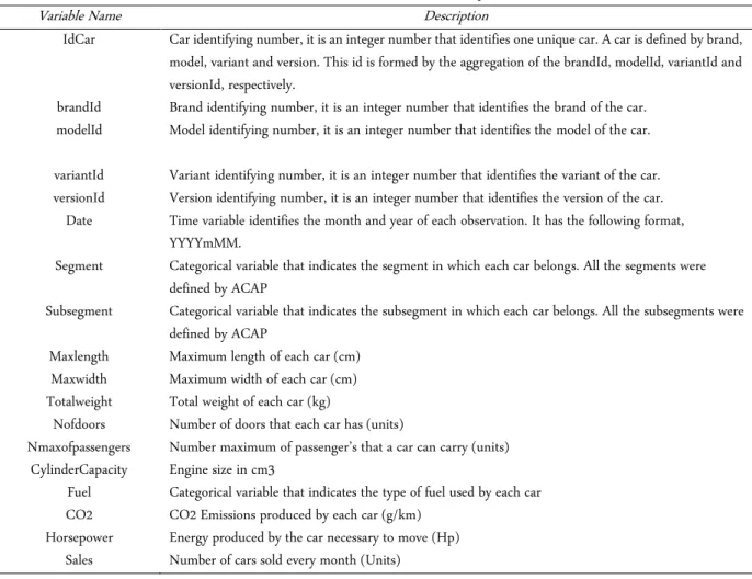
As previously said, the dataset starts in January 2008 and ends in July 2018 and is presented on a monthly frequency. The vehicle description variables, which are characteristics of the car, are presented in the table below. This information was provided by ACAP, therefore no caution measures were taken regarding the reliability of the data.
Table 1: Variable identification and Description
Variable Name Description
IdCar Car identifying number, it is an integer number that identifies one unique car. A car is defined by brand, model, variant and version. This id is formed by the aggregation of the brandId, modelId, variantId and versionId, respectively.
brandId Brand identifying number, it is an integer number that identifies the brand of the car. modelId Model identifying number, it is an integer number that identifies the model of the car. variantId Variant identifying number, it is an integer number that identifies the variant of the car. versionId Version identifying number, it is an integer number that identifies the version of the car.
Date Time variable identifies the month and year of each observation. It has the following format, YYYYmMM.
Segment Categorical variable that indicates the segment in which each car belongs. All the segments were defined by ACAP
Subsegment Categorical variable that indicates the subsegment in which each car belongs. All the subsegments were defined by ACAP
Maxlength Maximum length of each car (cm) Maxwidth Maximum width of each car (cm) Totalweight Total weight of each car (kg)
Nofdoors Number of doors that each car has (units)
Nmaxofpassengers Number maximum of passenger’s that a car can carry (units) CylinderCapacity Engine size in cm3
Fuel Categorical variable that indicates the type of fuel used by each car CO2 CO2 Emissions produced by each car (g/km)
Horsepower Energy produced by the car necessary to move (Hp) Sales Number of cars sold every month (Units)
Besides the information provided by ACAP two more variables were created which were ISV and the lag of the variable Sales. At this point, the dataset has 514.988 observations. In this population of passenger cars, there are 16.752 different vehicles, 48 brands, 596 car models, 2.625 car variants.
15 Table 2: Descriptive Statistics on the Data Set
Variable Name Number of Observations Mean Std. Dev. Min Max Distaxestotheleft 115,207 2,629.37 203.29 978 6,450 Maxlength 21,751 4,497.98 250.89 3,620 5,370 Maxwidth 21,702 1,843.26 84.49 1,590 2,085 Totalweight 127,877 2,007.02 605.29 3 6,750 Nofdoors 514,964 4.36 0.98 2 7 Nmaxofpassengers 447,832 4.94 0.69 2 9 CylinderCapacity 514,988 1,810.36 722.59 0 6,752 CO2 513,887 137.49 41.97 0 547 Horsepower 514,945 108.04 59.80 20 658 ISV 510,231 6,308.10 7,072.36 100 70,344.68 Sales 514,988 3.61 16.83 0 913
As we can see, not all the variables have values in the 514,988 observations. Regarding the maximum length of a passenger car, on average, is 4,500 cm with 21,751 observations which represent 95.8% of missing values. The maximum width of a passenger car, on average, is 1,843 cm with 21,702 observations which represent 95.8% of missing values.
The total weight of a car, on average, is 2,007 kg with a minimum of 3 kg and a maximum of 6,750 kg. Despite being the lowest value possible for the weight of a car, it is not expectable that 3 kg is the actual weight. Hence this error might be a typing error in ACAP’s Information System.4 This variable has a percentage of missing values of around 75.1%.
On average, the number of doors of a passenger car is 4, with a minimum of 2 and maximum of 7. Despite this indicator, in our sample, roughly 65% of the passenger cars have 5 doors.
The maximum number of passengers that a passenger car can take is between 2 and 9, where the average is 5 passengers. Based in our sample, on average, a passenger car in Portugal has 1,806 cm3 of cylinder capacity and produce 137 grams of CO2 per kilometer. Due to electric cars, the lowest possible value for these two variables is 0 (zero). By law, the minimum tax
4 If a subsample is created, only with the observations where total weight of a car is less than 500 kg, the subsample has 307 observations where the mean is 30.7 kg the minimum is 3 kg and the maximum is 135 kg.
16 charged by car is 100€ and throughout the years, each passenger car identified by a unique IdCar pays, on average, 6309€ of ISV.
Since this study is focused on sales, these descriptive statistics are important, from the previous table, on average and per IdCar, the number of vehicles sold is around 3 units. Since the IdCar variable is disaggregated until the version of the car, it can be concluded that, per car version, on average, the number of cars sold is 3 units. From the previous table, the maximum number of cars sold by a specific IdCar is almost 1,000 units, whereas the minimum value is 0.
The next analysis will be focused on the different passenger car segments, which were all defined by ACAP. The information presented on each individual segment will be based on Appendix XII and XIII. From our sample, the major segments of passenger cars in Portugal are Medium Family and Big Family, together they represent around 49% of the passenger cars in Portugal while the second biggest segment in Portugal is the Utilitarian Car which represents 22.5%. This numbers align with the average of number of doors (4) and with the average of the maximum number of passengers (5).
According to our sample, the two most used fuels in the Portuguese market are gasoline and diesel (Appendix XIV and XV). As previously said, diesel is used on 62% of the total passenger cars, together with Gasoline, they represent more than 97% of the market. Nowadays, the environmental advantages of the electric cars are known but the market penetration has been slow. The electric vehicles, according to our sample, do not have a relevant place in the market with a market share of 0.4%, if all cars with an electric component are considered the market share increases to 2.17%.
5. Methodology/Model
To explain the effect of the ISV in the sales of new Portuguese passenger vehicles, for every variable, an individual fixed model will be estimated to understand how each individual
17 variable affects the sales of the passenger cars. Afterwards, other models will be estimated in order to see how each variable interact with the remaining ones. For estimation purposes a new IdCar was built with the BrandId, ModelId and VariantId. The consequence of this
transformation was the aggregation of the variables Sales (sum) and ISV (average), by the new IdCar, year and month.
The main fixed effect model combines all the previous individual effects. The dependent variable is the logarithm of the number of cars sold in each month, the explanatory variables are the logarithm of the ISV, the lag of the dependent variable, year and month dummy variables. The ISV was chosen to be included in the model since the objective of this study is to see how this specific tax affects the sales of passenger cars in the Portuguese market. In general, the trend component is highly significant for products and services, therefore, a lag of the dependent variable was included in the model. Regarding the month and year dummy variables, they were included in the model with the purpose of capturing macroeconomic impacts that might influence the dependent variable. Therefore, the model estimated is presented below, Equation 4:
𝒍𝑺𝒂𝒍𝒆𝒔𝒊,𝒕= 𝜷𝟏𝒍𝑰𝑺𝑽𝒊,𝒕+ 𝜷𝟐𝒍𝑺𝒂𝒍𝒆𝒔𝒊,𝒕−𝟏+ ∑ 𝜹𝒋 𝒎𝒐𝒏𝒕𝒉𝒋+ ∑ 𝜹𝒛 𝒚𝒆𝒂𝒓𝒛 𝟏𝟎 𝒛=𝟏 𝟏𝟐 𝒋=𝟏 + 𝜶𝒊+ 𝒖𝒊𝒕
𝑗 = 2, … ,12 𝛿𝑗 represents dummy variables, equals 1 for each month 𝑧 = 2009, … ,2018 𝛿𝑧 represents dummy variables, equals 1 for each year,
starting in 2008
𝑙𝑆𝑎𝑙𝑒𝑠𝑖,𝑡 represents the log number of vehicles i sold in time period t ; 𝑙𝐼𝑆𝑉𝑖,𝑡 is the log amount paid by the vehicle i in time period t ; 𝑙𝑆𝑎𝑙𝑒𝑠𝑖,𝑡−1 represents the log number of vehicles i sold in time period t-1;
For every year and month, a dummy variable was created, omitting one in the estimations in order to avoid multicollinearity problems, for the year dummy variables the base group is 2008 and for the month dummy variables the base group is January. Through this
18 method it will be obtained a year fixed effect and a month fixed effect on the sales of passenger cars.
For this model to be accurate the variables must have time variability, otherwise the impact of the variables will be removed. The ISV and the lag of the dependent variable for each vehicle must change over time, regarding the ISV, this variability is accomplished due to the Government changes in the tables of the Cylinder component and the CO2 component. This government changes give a source of external variations that can be used to identify the causal effect. Since sales are not constant over time, there is no concern regarding this subject. To study the possibility of an anticipation effect, the following model was estimated, Equation 5:
𝒍𝑺𝒂𝒍𝒆𝒔𝒊,𝒕= 𝜷𝟏∆𝒍𝑰𝑺𝑽𝒊,𝒕+ ∑ 𝜹𝒛 𝒚𝒆𝒂𝒓𝒛 𝟏𝟎
𝒛=𝟏
+ 𝜶𝒊+ 𝒖𝒊𝒕
𝑧 = 2009, … ,2018 𝛿𝑧 represents dummy variables, equals 1 for each year, starting in 2008
The changes performed in the ISV, in most cases, are made in January since it is when the Government budget is published, therefore the estimation will be conditional on January. The model presented has as dependent variable, the logarithm transformation of the cumulative sales on a monthly basis, it will also contain the year dummy variables in order to isolate macroeconomics effects that might impact this effect.
6. Results
In this section it will be presented the main conclusions regarding the analysis performed. The sales weighted average of the ISV indicates that the average ISV has been decreasing, from 4200€ in 2008 to 2600€ in 2017. (Appendix XVI). As happened in Norway and Switzerland, the sales weighted-average of the CO2 emissions have been decreasing significantly, in 2008 the average was 140 g/km and in 2017 was 105 g/km (Appendix XVII). There is also a shift of the Portuguese consumer towards lower CO2 emission vehicles. In 2008,
19 more than 90% of the vehicles bought had CO2 emissions between 91 and 200 g/km while in 2017, more than 90% of the vehicle bought had CO2 emissions between 51 to 150 g/km (Appendix XVIII).The unit tax and the parcel to subtract have increased by the Portuguese Government, hence this decrease in the ISV can be explained mainly by the efficiency increase in the CO2 emissions of the vehicles , the general decrease of the vehicles engine sizes (Appendix XIX) and the shift of the consumer preferences for vehicles that are more environmentally friendly.
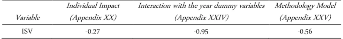
The table below presents the estimates of the ISV in the several models assessed. Table 3: ISV Coefficients in the different models
Variable Individual Impact (Appendix XX) Interaction with the year dummy variables (Appendix XXIV) Methodology Model (Appendix XXV)
ISV -0.27 -0.95 -0.56
Ahead it will be discussed the individual impact of the variables included in the model. Starting with the ISV tax, as any other tax, it is expected to have a negative impact. Based on the previous table, it is observable that the ISV is a statistically significant variable, if the ISV increases 1%, the sales of new passenger vehicles will decrease, on average, by 0.27%.
Concerning the individual impact of the lag of the dependent variable (Appendix XXI), it is expected that the sales of the current period are significantly affected by the sales of the previous one. It can be seen, through R-Squared, the lagged dependent variable explains 72% of the variations of the new passenger cars sales. If the sales of the past month increase 1%, on average, the sales of the current month will increase 0.56%.5
Regarding the year dummy variables, the base year is 2008. According to Appendix XXII, all the coefficients signs are negative, this means, all the year dummy variables captured macroeconomic effects that will impact the sales of new passenger cars negatively. Until 2013,
5 The fixed effect model does not allow the lagged dependent variable to be added to the model since it will lead
20 the coefficients have been decreasing, from that moment on, the coefficients increased becoming less negative throughout the years. This is not possible to confirm in 2018 since the data collected does not correspond to the full year.
The base group in the monthly dummy variables is January. From Appendix XXIII, it can be concluded that the impact in the first semester of the year is higher than in the second semester, since the coefficients are higher in the first semester. This is particularly true for March, May and June where there is a sales increase around 24%6, 17%7 and 23%8, respectively when compared to January. On the other hand, in August, on average, there is a relevant decrease of 16%9 and a small decrease in September when compared to January. On the second semester of the year, the effect in sales appear to be on the same level of January since the coefficients are smaller.
A model containing the year dummy variables and the ISV was estimated, when compared to the model used to see the individual effects the coefficient of the ISV kept the negative influence but increased to -0.95%. The year dummy variables might capture other macroeconomic effects that the ISV can not capture by itself. Therefore, after the introduction of the year dummy variables part of those effects is included in the ISV coefficient. Therefore, for robustness reasons the year dummy variables and month dummy variables will be included in the next estimations.
A full model containing only the fixed effects was estimated, with the variables log of the ISV, lag of the variable lSales, month and year dummies. Regarding the ISV coefficient, it decreased to -0.56% when compared to the model Interaction of the ISV with year dummy variables. The lag of the dependent variable, lSales decreased significantly its size to 0.49 when compared to the individual effect of the lag of the dependent variable.
6 100*(exp(0,2174777)-1)= 24.29% from Appendix XXIII 7 100*(exp(0,1612128)-1)= 17,49% from Appendix XXIII 8 100*(exp(0,2044038)-1)= 22.68% from Appendix XXIII 9 100*(exp(-0,169064)-1) = -15.55% from Appendix XXIII
21 All the year dummy variables have a lower coefficient when compared to the individual impact of the year dummy variables model. This decrease in the coefficients of the year dummy variables and the lag of the dependent variable can be explained since the effects that were previously captured by these variables are now being included in the month dummy variables. Most of the changes occurred in the month dummy variables, in the first semester of the year, the coefficients increased their size, therefore their effect is more significant. The months with a relevant change were February, increased from 3%10 to 15%11, March increased its positive significance from 24% to 40%12, August decreased its negative size from -16% to -19.54%13. On the other hand, the coefficients of the second semester kept relatively stable, when compared to the model individual effects of the month dummy variables.
This model, when compared to individual effect of the lag of the dependent variable, has a lower overall R-Squared, 0.56 and 0.73, respectively. Therefore, if the scope of this dissertation was to simply explain the sales of passenger cars in Portugal, this should be a result to be taken into consideration. In the first analysis performed, it was considered the possibility of an anticipation effect regarding the changes in the ISV.
A sales anticipation effect is a change of the consumer behavior before any structural change or values used to calculate the ISV. Figure 1 was built with the intention to validate that idea, what this figure shows is how the sales of the previous periods are affected by the current ISV. For that idea to be confirmed, at some point in the previous periods, the expectations had to be none, in practical terms, this means that at some point the ISV coefficient had to be zero.
10 100*(exp(0.0295313)-1) = 3.00% from Appendix XXIII 11 100*(exp(0.1266291)-1) = 14.99% from Appendix XXV 12 100*(exp(0.3379839)-1)= 40.21% Appendix XXV 13 100*(exp(-0.2170206)-1) = 19.54% Appendix XXV
22 From figure 1, it can be seen that in the Portuguese market there is a relevant sales anticipation effect with a positive impact. Before the changes made in the ISV, at time T, there is a positive increase in the sales of passenger vehicles around 0.25% and the period immediately after, the impact is negative, -0.05%. Six months prior to the change, this effect reaches is maximum positive impact with a size of 0.365% and after six months of the changes made in the vehicle registration tax, its negative impact increases significantly reaching a maximum of -0.378% after 12 months. To see the inputs of this figure, see Appendix XXVI.
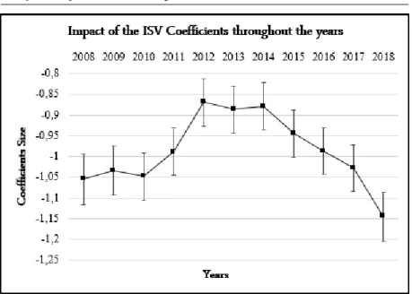
Based on Figure 2, an analysis was performed with the intention to see if the effect of the ISV was constant throughout the years. Since 2008, the coefficients of the ISV have been decreasing until 2012, from that year on, their size has been increasing every year. In 2012, a change of 1% in the ISV will cause a decrease, on average, 0.86% of the sales of new passenger cars. Based on or sample, the ISV never had an impact like in 2018, with a coefficient of -1.14%.
Figure 1– Validation of a possible Anticipation Effect. Coefficient of the first difference of the ISV in the sales of passenger cars in Portugal; Dependent Variable: Log of the variable Sales from 2008 to 2018. Regression estimated, Equation 2 (includes year dummy variables and only for month= January):
23 7. Conclusion
As previously said, the main goal of this research is to evaluate how the ISV tax impact the sales of new passenger cars in Portugal. The impact of the ISV is sensitive to add and drop of variables that capture those same effects, that is why the effect of the ISV increases to -0.95% when the time year dummy variables are included in the model but decreases to -0.56% when the lag of the dependent variable is incorporated. This changes in the ISV coefficient may occur because the models Interaction of the ISV with the year dummy variables and Interaction of all the effect may not estimate correctly the causal effect due to endogeneity problems therefore the effect of the ISV in the sales of new passenger vehicles is 0.27%. This endogeneity problem arises because there might be a correlation between certain unobserved factors at the vehicle level and the changes of the ISV.
The lag of the sales of passenger cars, besides having a strong impact and being significant, when introduced in the model gives the model a better fit. When introduced in the model, the fit of the model increases significantly, this means if the goal was to explain only the sales of passenger in the Portuguese market then the trend component should be improved. The sales of passenger cars in the Portuguese market are more significant in the first semester of the year than in the second semester. The month March has the most positive significant
Figure 2 – Effect of the logarithm of the ISV in the sales of passenger cars through the years; Dependent Variable: Log of the variable Sales from 2008 to 2018
24 impact in the sales of passenger cars, on the other hand, August has the most negative significant impact in the sales of new passenger cars in Portugal. For the past decade, the sales of passenger cars have been suffering changes due to macroeconomic effects, those effects had the worst impact in 2013. As the years pass, the negative impact of the year dummy variables increases until 2013, from that moment on, their effect suffered a weak decrease.
It can also be concluded that there is a positive sales anticipation effect with an impact between 0.2% and 0.4%, 6 months prior to the changes of the ISV this effect reaches his highest positive impact and 12 months after the changes in the ISV this effect reaches his highest negative impact.
Regarding the fact that the impact of the ISV has not been constant throughout the years. The ISV had the highest impact in 2008 and in 2018, on the other hand, in 2012 the ISV had the lowest significance.
The environmental impact of the changes made were briefly studied, the average of the CO2 emissions of the new passenger vehicles has been decreasing, accompanied by a decrease in the engine size which lead to a significance decrease of the average ISV paid.
25 References
Alberini, A., & Bareit, M. (2016). The Effect of Registration Taxes on New Car Sales and Emissions : Evidence from Switzerland, (August).
Ciccone, A. (2015). Environmental effects of a vehicle tax reform: empirical evidence from Norway, (February).
Eurostat. (2018). Passenger cars in the EU. Retrieved from
https://ec.europa.eu/eurostat/statistics-explained/pdfscache/25886.pdf
Pellizzari, M. (2005). Notes on Panel Data and Fixed Effects models, 1–18. Retrieved from http://didattica.unibocconi.it/mypage/dwload.php?nomefile=FIXEDEFFECTS20100421 123407.PDF
I Appendix
Appendix I - Total Tax Revenues in Portugal in 2017 Source: ACAP, DGO e ENMC
Appendix II - Tax Revenues of 2017 related to the Automobile Industry in Portugal, millions of euros Source: ACAP, DGO e ENMC
II Appendix IV - Data Treatment (Continuation)
A problem that is common in dealing with data sets is the missing values. The dataset provided by ACAP uses zeros instead of missing values. The solution found to this problem was removing those zeros, variable by variable, the exception for this rule was the variable sales. The special cases that were found are related with electric cars. In the case of electric cars, the variables cylinder capacity and CO2 will represent an actual zero instead of missing values, this happens because the engine of electric cars does not have cylinders hence, they do not have cylinder capacity. The production of CO2 emissions by electric cars is assumed to be zero as well, therefore in the cases presented before those zeros were kept in the dataset. This is particularly important to handle since it will lead to the bias of certain variables.
III Ap pe nd ix V : Agg re ga tion of th e C yli nde r C ap acit y T ab le, s tart ing in 20 08
IV Ap pe nd ix VI : Agg re ga tion of th e C O2 Ta bles, f or g asol ine cars , s tarti ng in 2 008
V Ap pe nd ix VI I: Agg re ga tion of th e C O2 Ta bles, f or die sel cars , start ing in 2 00 8
VI Appendix VIII: Intermediate rates applied in the calculations of the ISV, starting in
2008
Appendix IX: CO2 emissions intensity, comparison between Diesel and Gasoline vehicles, starting in 2008
Appendix X: Sales Weighted Average of the ISV paid by Diesel and Gasoline Vehicles, starting in 2008
VII Appendix XI: Diesel and gasoline cars sold in units, starting in2008
Appendix XII: Vehicle Division by Car Segment
Segment Frequency Absolute Frequency Relative Cumulative Frequency
A 31,561 6.13 6.13 B 115,799 22.49 28.61 C 152,339 29.58 58.20 D 99,245 19.27 77.47 E 32,551 6.32 83.79 F 18,429 3.58 87.37 G 31,272 6.07 93.44 H 33,792 6.56 100.00 Total 514,988 100.00
Appendix XIII: Segments mentioned in Appendix XII
Segment Name Description
A City
Specially designed to be used in urban areas, due to its small size is very good for parking. It is efficient and usually cheap.
B Utilitarian
Bigger than the average passenger car, usually designed to make a specific task better than a passenger car.
C Family Medium
This type of vehicles can take until 5 passengers. It is commonly referred to the normal size vehicles.
D Family Big
The main difference when compared to the vehicles of the previous segment is the size, usually they are bigger.
E Superior
This type of vehicle is bigger and more luxurious than a large family cars. Also known as medium luxury vehicles.
VIII
F Luxury
High quality vehicles associated to well-known brands. It is comfort but also has a very good performance and design. G Sports Utility Vehicle
This type of vehicles can be drive on road and off road. They have less space for luggage and for passengers.
H Multi Purpose Vehicles
This type of vehicles has an higher rooftop but a more flexible and larger interior when compared to family cars.
Appendix XIV: Descriptive Statistics about the Fuel used in Passenger cars Fuel Frequency Absolute Frequency Relative Cumulative Frequency
D 319,477 62.04 62.04 D/E 1,205 0.23 62.27 E 2.073 0.40 62.67 EREV 110 0.02 62.69 G 180,529 35.05 97.75 G/E 6,297 1.22 98.97 G/GN 275 0.05 99.02 G/GPL 3425 0.67 99.69 GPL 60 0.01 99.70 PHEV 1,537 0.30 100.00 Total 514,988 100.00
Appendix XV: Description of the Fuel mentioned in Appendix XIV
Fuel Description
D Car that uses Diesel as source of internal engine
D/E Hybrid car, uses Diesel in the internal engine but also Electric engine E Car that uses Electric power as source of internal engine EREV
Extended-range electric vehicles (EREV) uses an internal combustion engine but also has an electric motor. The EREV vehicles have a plug-in battery pack, if goes out of energy the internal combustion engine charges it again. G Car that uses Gasoline as source of internal engine
G/E Hybrid car, uses Gasoline in the internal engine but also Electric engine
G/GN Car that uses GN (Natural Gas) as the source of the internal engine but also, gasoline in the start G/GPL Car that usesLiquefied Petroleum Gas as source of the internal engine but also, gasoline in the start
GPL Car that uses exclusively GPL (Liquefied Petroleum Gas) as source of internal engine PHEV
Plug-In Hybrid Electric Vehicles (PHEV) is an hybrid car that uses an electric motor and an internal combustion engine. PHEV batteries can be charged by plugging into an external source of electric power.
IX Appendix XVI: Sales Weighted Average of ISV, starting in 2008
Appendix XVII: Sales Weighted Average of CO2 Emissions throughout the years
X Appendix XX: Individual Effect of the ISV – Regression Output
Description: With this regression the objective is to see the individual effect of the ISV in the sales of passenger cars; The regression estimated was
𝑙𝑆𝑎𝑙𝑒𝑠𝑖,𝑡 = 𝛽0+ 𝛽1𝑙𝐼𝑆𝑉𝑖,𝑡 + 𝑢𝑖,𝑡
R-Squared
Within 0.0013 Between 0.1644 Overall 0.1093
Variables Coefficient Standard Error t-Statistic
Constant 4.0 0.2 17.87
lISV -0.27 0.03 -9.66
Appendix XXI: Individual Effect of the Lag of Dependent Variable – Regression Output Description: With this regression the objective is to see the individual effect of the lag of the dependent variable in the sales of passenger cars; The regression estimated was
𝑙𝑆𝑎𝑙𝑒𝑠𝑖,𝑡 = 𝛽0+ 𝛽1𝑙𝑆𝑎𝑙𝑒𝑠𝑖,𝑡−1 + 𝑢𝑖,𝑡
R-Squared
Within 0.3062 Between 0.9446 Overall 0.7332
Variables Coefficient Standard Error t-Statistic Appendix XIX: Average of the Cylinder Capacity of the Passenger vehicles in cm3
XI
Constant 0.967 0.008 119.63
L.lSales 0.557 0.003 163.31
Appendix XXII: Individual Effect of the Year Dummy Variables – Regression Output Description: With this regression the objective is to see the individual effect of year dummy variables in the sales of passenger cars; The base group is 2008. The regression estimated was
𝑙𝑆𝑎𝑙𝑒𝑠𝑖,𝑡 = 𝛽0+ 𝛿12009 + (… ) + 𝛿102018 + 𝑢𝑖,𝑡
R-Squared
Within 0.1081 Between 0.0053 Overall 0.0025
Variables Coefficient Standard Error t-Statistic
Constant 2.81 0.01 206.61 i.year 2009 -0.43 0.02 -27.70 2010 -0.46 0.02 -28.24 2011 -0.86 0.02 -49.22 2012 -1.37 0.02 -75.74 2013 -1.42 0.02 -77.70 2014 -1.30 0.02 -71.04 2015 -1.22 0.02 -65.88 2016 -1.12 0.02 -59.54 2017 -1.15 0.02 -60.52 2018 -1.11 0.02 -53.08
Appendix XXIII: Individual Effect of the Month Dummy Variables – Regression Output Description: With this regression the objective is to see the individual effect of the month dummy variables variable in the sales of passenger cars; The base group is January. The regression estimated was
𝑙𝑆𝑎𝑙𝑒𝑠𝑖,𝑡 = 𝛽0+ 𝛿1𝐹𝑒𝑏𝑟𝑢𝑎𝑟𝑦 + (… ) + 𝛿10𝐷𝑒𝑐𝑒𝑚𝑏𝑒𝑟 + 𝑢𝑖,𝑡
R-Squared
Within 0.0141 Between 0.0017 Overall 0.0026
Variables Coefficient Standard Error t-Statistic
Constant 1.80 0.01 171.53
i.month
XII March 0.22 0.01 14.69 April 0.09 0.01 5.85 May 0.16 0.01 10.91 June 0.20 0.01 13.81 July 0.11 0.01 7.57 August -0.17 0.02 -10.89 September -0.03 0.02 -1.82 October 0.02 0.02 1.26 November 0.02 0.02 1.17 December 0.05 0.02 3.14
Appendix XXIV: Interaction of the Year Dummy Variables and the ISV– Regression Output Description: With this regression the objective is to see the interaction of ISV and the year dummy variables in the sales of passenger cars; The base group is 2008. The regression estimated was
𝑙𝑆𝑎𝑙𝑒𝑠𝑖,𝑡 = 𝛽0+ 𝛿12009 + (… ) + 𝛿102018 + 𝑢𝑖,𝑡
R-Squared
Within 0.1231 Between 0.1366 Overall 0.1166
Variables Coefficient Standard Error t-Statistic
Constant 10.7 0.2 46.15 lISV -0.95 0.03 -34.10 i.year 2009 -0.43 0.02 -28.07 2010 -0.48 0.02 -29.76 2011 -0.90 0.02 -52.18 2012 -1.41 0.02 -78.63 2013 -1.52 0.02 -82.75 2014 -1.46 0.02 -77.44 2015 -1.39 0.02 -73.05 2016 -1.22 0.02 -64.66 2017 -1.28 0.03 -66.28 2018 -1.22 0.03 -57.89
XIII Appendix XXV: Interaction of all the effects – Regression Output
Description: With this regression the objective is to see how all these variables interact. The base group are 2008 and January. The regression estimated was the one presented in the Methodology
R-Squared
Within 0.3671 Between 0.6203 Overall 0.5626
Variables Coefficient Standard Error t-Statistic
Constant 6.2 0.2 27.16 lISV -0.56 0.03 -20.49 L.lSales 0.494 0.004 139.60 i.year 2009 -0.27 0.01 -17.85 2010 -0.29 0.02 -17.97 2011 -0.59 0.02 -34.15 2012 -0.87 0.02 -47.34 2013 -0.88 0.02 -46.45 2014 -0.86 0.02 -44.35 2015 -0.84 0.02 -43.20 2016 -0.73 0.02 -38.56 2017 -0.80 0.02 -41.07 2018 -0.81 0.02 -37.74 i.month February 0.13 0.01 8.95 March 0.34 0.01 23.93 April 0.05 0.01 3.60 May 0.22 0.01 15.50 June 0.23 0.01 16.10 July 0.08 0.01 5.98 August -0.22 0.01 -14.88 September 0.12 0.01 8.36 October 0.11 0.01 7.35 November -0.05 0.01 3.44 December 0.10 0.01 6.74
XIV Appendix XXVI: Anticipation effect validation
Description: The purpose of this regression is to confirm the existence of an anticipation effect. Inputs for figure 1
Time Operator Coefficient
T-12 0.133 T-11 0.249 T-10 0.194 T-9 0.174 T-8 0.256 T-7 0.270 T-6 0.365 T-5 0.315 T-4 0.218 T-3 0.278 T-2 0.258 T-1 0.233 T -0.055 T+1 -0.078 T+2 -0.063 T+3 -0.021 T+4 -0.044 T+5 -0.029 T+6 -0.029 T+7 -0.165 T+8 -0.202 T+9 -0.255 T+10 -0.297 T+11 -0.300 T+12 0.378