Wave climate in a global warming scenario: simulations with a CMIP5 ensemble

(1)

UNIVERSIDADE DE LISBOA FACULDADE DE CIÊNCIAS

DEPARTAMENTO DE ENGENHARIA GEOGRÁFICA, GEOFÍSICA E ENERGIA

Wave climate in a global warming scenario: simulations with a

CMIP5 ensemble

Gil Lemos

Mestrado em Ciências Geofísicas Meteorologia

Dissertação orientada por: Prof. Dr. Álvaro Semedo

Prof. Dr. Pedro Miranda

(2)

iii

Resumo

As ondas gravíticas geradas pelo vento na superfície do oceano são as mais energéticas do espectro, sendo responsáveis por mais de metade da energia presente em todas as ondas nesta superfície (Kinsman, 1965). São geradas pela transferência de momento do vento para a água e dominam o espectro de ondas oceânicas, ultrapassando a contribuição das marés, das “storm surges”, dos tsunamis, etc. (Munk, 1951). Pela sua prevalência no oceano e influência nas actividades humanas, o seu estudo deve ser aprofundado, e as potenciais alterações no seu regime devem ser tidas em conta. Porém, apesar da sua relevância, não existe ainda nenhum modelo teórico preciso de geração e crescimento das ondas, dado que os mecanismos presentes nestes fenómenos não são ainda totalmente compreendidos por forma a serem correctamente quantificados.

Quando o vento sopra sobre a superfície do oceano, ondas são formadas pela transferência de momento no sentido da água. Esta perturbação inicial pode desenvolver-se se o vento continuar a soprar de forma constante, sendo que as ondas irão crescer até atingirem o seu nível de saturação. Os dois principais tipos de ondas à superfície do oceano são denominados “wind sea” ou apenas “sea”, e “swell”. As ondas de “sea” detêm alta frequência e curtos comprimentos de onda, estando directamente associadas ao campo de vento sobrejacente, crescendo rapidamente e depressa atingindo o nível de saturação. Por sua vez, as ondas de “swell”, com frequências mais baixas e comprimentos de onda maiores, crescem lentamente e podem propagar-se com velocidades de fase superiores à velocidade do vento, uma vez que também extraem energia de ondas com mais alta frequência, devido a interações não lineares entre as ondas. Estas ondas podem propagar-se por milhares de quilómetros (Barber and Ursell, 1948; Munk et al., 1963; Snodgrass et al., 1966) com muito ligeira atenuação (Ardhuin et al., 2009). Assim sendo, é possível assumir que existe uma ligação causal entre, por exemplo, um evento local de erosão costeira e uma tempestade que ocorreu “do outro lado” do mundo (em outro hemisfério). Este é apenas um dos factores interessantes que motivam a execução deste trabalho de análise das futuras alterações no clima de ondas global, uma vez que as alterações climáticas atmosféricas locais no vento podem propagar-se sob a forma de ondas à superfície do oceano, e gerar impactos a longas distâncias.

Até recentemente, o impacto das alterações climáticas no clima de ondas futuro tinha recebido muito pouca atenção. Nos últimos anos, alguns estudos foram realizados, sob os auspícios do COWCLIP (Coordinated Ocean Wave Climate Project), utilizando um único

(3)

iv

modelo e um único cenário de concentração de gases de efeito estufa (CMIP3), recebendo atenção moderada por parte do IPCC-AR5 (Intergovernmental Panel for Climate Change - Fifth Assessment Report). No presente estudo, o impacto do aquecimento global no clima de ondas global é investigado, através de um “ensemble” composto por 2 membros (simulações do modelo de ondas WAM) de um conjunto maior, composto por 8 simulações dinâmicas e 20 simulações estatísticas, denominado GLOWAVES-2, e pertencente ao projecto COWCLIP. O (único) forçamento destas duas simulações (em termos de velocidade do vento e cobertura oceânica de gelo) provém do modelo climático EC-Earth, seguindo um cenário de elevadas emissões de gases de efeito estufa (RCP8.5). Ambas as simulações cobrem um período total de 130 anos (1971-2100), no entanto, para efeitos de análise comparativa, dois períodos mais curtos são utilizados como referência: o “clima presente” (PC20: média das duas simulações (PC20-1 e PC20-4); 1971-2000) e o “clima futuro” (projectado; FC21: média das duas simulações (FC21-1 e FC21-4); 2071-2100). O período de referência histórico (1971-2005) foi validado através da comparação com a reanálise ERA-Interim, do ECMWF (European Centre for Medium-Range Weather Forecasts) e com dados observacionais de bóias, revelando que o modelo WAM, com forçamento do EC-Earth, é capaz de produzir cenários realistas do clima de ondas global no final do século XX, fornecendo a confiança necessária na capacidade de simular uma alteração climática igualmente credível até ao final do século XXI. Os resultados (alterações futuras no clima de ondas como projectado pelas simulações) são obtidos através da comparação entre as médias de PC20 e FC21, para quatro variáveis diferentes: (altura significativa; m), (período médio da onda; s), (direcção média da frente de onda; º), (potência das ondas; W/m, = , como em Young, 1999). Para complementar os resultados destas variáveis, os impactos da alteração climática no campo do vento ( ; velocidade do vento a 10 metros de altura; m/s)

foram também analisados. Os resultados expõem médias a nível anual e sazonal (estações extremas de Inverno e Verão: DJF (Dezembro, Janeiro e Fevereiro) e JJA (Junho, Julho e Agosto)). Como forma de complemento, são também apresentadas as tendências lineares ao longo do período 2006-2100, para a altura significativa e para a potência (fluxo de energia) das ondas.

Devido às alterações climáticas, as projecções indicam alterações estatisticamente significativas em todas as variáveis analisadas, que poderão referir-se a aumentos ou decréscimos na sua intensidade, gradiente espacial ou mudanças na localização geográfica de determinados valores. No que toca à altura significativa, , os aumentos nesta variável

(4)

v

dominam as projecções, essencialmente a nível anual, e durante o período JJA (verificando-se em 73.93% do oceano global), sendo no Oceano Antárctico (“Southern Ocean”) que os maiores aumentos se verificam, estando esta situação directamente relacionada com uma intensificação projectada a nível da velocidade do vento ( ) na mesma área. A região onde os decréscimos projectados se mostram mais prevalecentes é no Oceano Atlântico Norte, em particular durante DJF. A tendência linear de altura significativa projectada durante o período 2006-2100 estabelece-se, a nível anual, em 0.41 cm/década.

No que toca ao período médio, , são esperados aumentos nos seus valores anuais e sazonais em praticamente todo o oceano global, excepto no Atlântico Norte e Pacífico Oeste durante DJF, e em maior extensão no verão boreal (JJA), em 87.48% da área de oceano global, em média. Tendo em conta os resultados para esta variável e para a altura significativa, uma vez que a potência das ondas ( ) depende destes, é esperado que o seu comportamento não se diferencie muito dos anteriormente referidos. É efectivamente o que acontece nas projecções de , onde se verifica um padrão de alterações muito semelhante ao da altura significativa, uma vez que as diferenças de apresentam valores reduzidos. Aumentos projectados de potência das ondas (que se observam em 81.43% do oceano global) alcançam os 30% no sector Índico do Oceano Antárctico (a sudoeste da Austrália), durante o inverno austral (JJA), sendo que o valor médio de incremento a nível global para esta estação se situa nos 7.18%. A tendência linear de potência das ondas projectada durante o período 2006-2100 estabelece-se, a nível anual, em 0.36 cm/década.

Relativamente à direcção média da frente de onda ( ), as projecções indicam a prevalência de rotações anti-horárias (contra os ponteiros do relógio) nas latitudes médias e altas de ambos os hemisférios, associadas ao deslocamento latitudinal positivo das tempestades para latitudes mais elevadas (Arblaster et al., 2011). Nas regiões tropicais e subtropicais, rotações positivas (no sentido dos ponteiros do relógio) são consistentes com uma maior contribuição de “swell” proveniente do Oceano Antárctico, especialmente durante o inverno austral (JJA), quando a sua “produção” é maior.

A análise de EOFs (“Empirical Orthogonal Functions”) para os campos de e no Oceano Atlântico Norte, em termos de alterações entre o clima presente (PC20) e o projectado para o futuro (FC21), relevou que é esperado um ligeiro enfraquecimento dos principais centros de acção de ambos os campos (redução da variabilidade), a nível anual. A nível sazonal, comportamento similar foi detectado para a altura significativa, porém, a nível de

(5)

vi

potência, um ligeiro fortalecimento dos seus centros de acção é esperado, com um deslocamento latitudinal positivo associado, de cerca de 2º. No entanto, deslocamentos da posição dos valores climatológicos máximos para latitudes mais elevadas não se verificam para o Atlântico Norte, apenas em algumas regiões do Oceano Antárctico.

(6)

vii

Abstract

Ocean surface wind waves are of outmost relevance for practical and scientific reasons. On the one hand, waves have a direct impact in coastal erosion, but also in sediment transport and beach nourishment, in ship routing and ship design, as well as in coastal and offshore infrastructures, just to mention the most relevant. On the other hand waves are part of the climate system, and modulate most of the exchanges that take place at the atmosphere-ocean interface. In fact waves are the “ultimate” air-sea interaction process, clearly visible and noticeable. Up until recently, the impact of climate change in future wave climate had received very little attention. Some single model single scenario global wave climate projections, based on CMIP3 scenarios, were pursued and received some attention in the IPCC (Intergovernmental Panel for Climate Change) AR5 (Fifth Assessment Report). In the present study the impact of a warmer climate in the global ocean future wave climate is investigated through a 2-member “coherent” ensemble of wave climate projections: single-model, single-forcing, and single-scenario. The two ensemble members were produced with the wave model WAM, forced with wind speed and ice coverage from EC-Earth projections, following the representative concentration pathway with a high emissions scenario 8.5 (RCP8.5). The ensemble historic period has been set for 1971 to 2005. The projected changes in the global ocean wave climate are analyzed for the 2071-2100 period. The ensemble historical period is evaluated trough the comparison with the European Centre for medium-range weather forecasts (ECMWF) ERA-Interim reanalysis, and buoy observations.

(7)

viii

Acknowledgements

Lots of great things have happened in my life during the months that I spent working on this final thesis. I recall myself almost a year ago, being firstly introduced to this new working environment, with serious and purely scientific methodologies, thinking of how great it would be to finally embrace this type of work. What I didn’t know at the time was how important and revolutionary this following year would be. How challenging, enjoyable and gratifying at the same time, to work in a field that I love, with some of the most kind and enlightened minds of the area.

I would like to express my gratitude to my family, friends and girlfriend, which unconditionally supported me during these months of hard work, giving me the motivation and confidence needed to reach the place that I am now.

My most sincere thanks to my co-supervisor Álvaro Semedo, for his dedicated guidance through this thesis and for sharing with me his extensive knowledge about waves, and the wave climate in particular. Also, a warm thank you word to all the postgraduate studies department personnel, at Escola Naval, for receiving me with open arms and great kindness.

Special thanks to my co-supervisor Pedro Miranda for his advices, patience, and most of all, for being the key-element who gave me the opportunity of working in this field, with all these extraordinary people.

My warm thanks also goes to the COWCLIP community, particularly to Arno Behrens and Joanna Staneva, from Helmholtz-Zentrum Geesthacht institute (Germany; former GKSS), for allowing me to use the WAM model simulations, and for co-authoring some of my first scientific works.

(8)

ix

List of Figures

Figure 1 – Buoys: the red dots represent the position of each buoy, numbered in accordance with its WMO (World Meteorological Organization) code identifications.

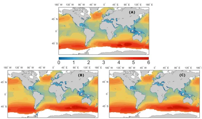
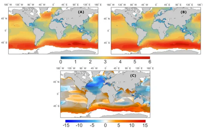
Figure 2 – Annual means of (m), 1979-2013 for (A) ERA-Interim, and 1971-2005 for (B) PC20-1 and (C) PC20-4.

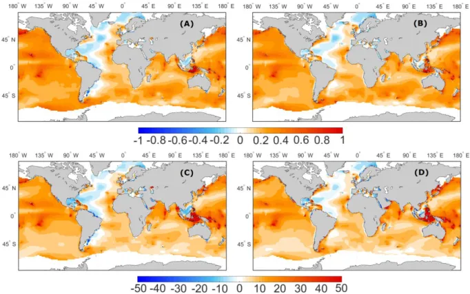
Figure 3 – anomalies (m) between simulations and reanalysis ((A), PC20-1, and (B), PC20-4) and the respective normalized differences (%) ((C), PC20-1, and (D), PC20-4).

Figure 4 – As in Fig. 2, but for (s).

Figure 5 – As in Fig. 3, but for (s).

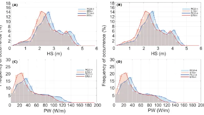
Figure 6 – Histograms and fit curves (%) of (A and B) (m) and (C and D) (W/m), computed from global annual means of PC20-1,4 (blue colored, blue lines) and ERA-Interim (red colored, red lines), for (A and C) 1 and (B and D) PC20-4. Overlaid histogram bars are gray colored.

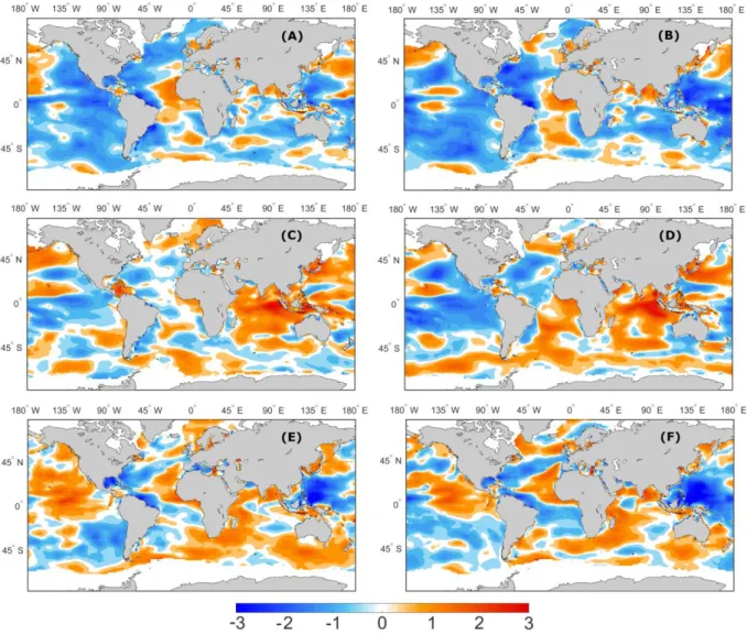
Figure 7 – Interannual ((A) and (B)) annual, ((C) and (D)) DJF and ((E) and (F)) JJA variability bias (dimensionless) between the PC20-1 (left) and PC20-4 (right), and ERA-Interim variances.

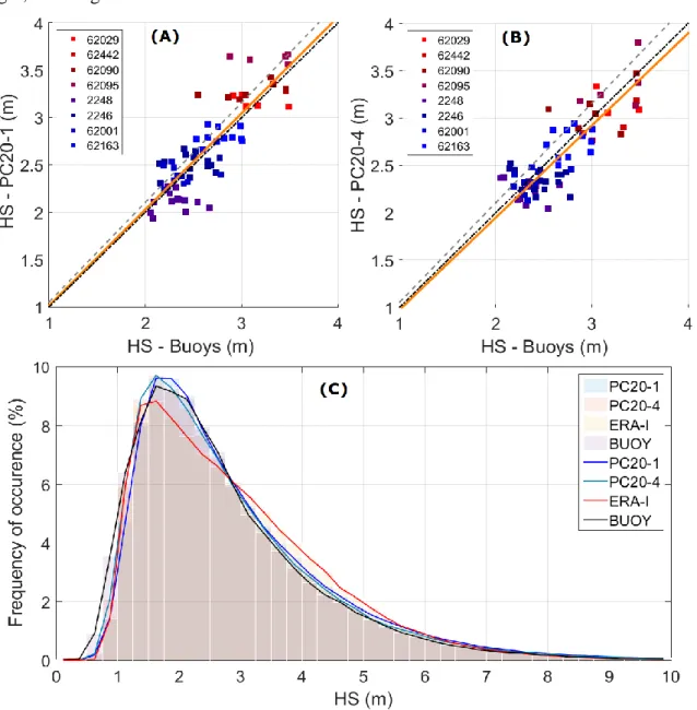
Figure 8 – Scatter-plots of buoys annual means (of at least 90% complete years) versus (A) PC20-1 and (B) PC20-4 annual means for the same location and yearspan, with linear fits (full orange lines; and from the comparison of buoys with ERA-Interim data: dashed gray lines). (C) Histogram and fit curve from buoy observations (black line), PC20-1,4 (blue and light blue lines) and ERA-Interim reanalysis data (red line). Overlaid histogram bars are gray colored.

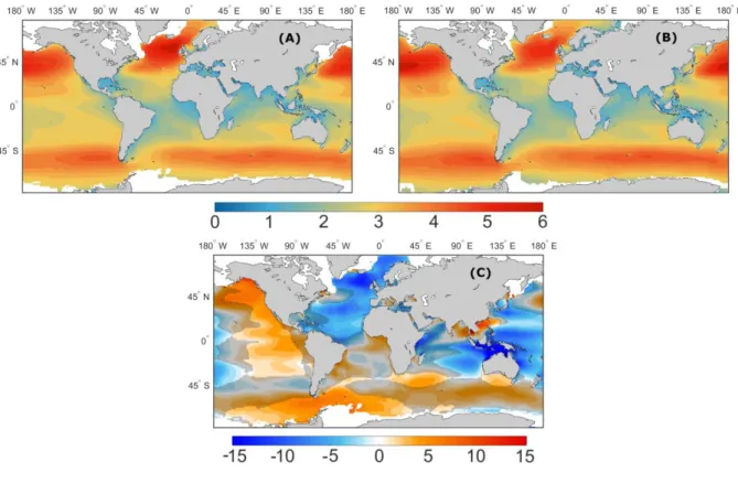
Figure 9 – Annual means of (m), for (A) PC20 and (B) FC21, and (C) normalized differences (%): FC21 minus PC20 normalized by PC20.

Figure 10 – As in Fig. 9, but for DJF.

(10)

xi

Figure 12 – (A) Annual, (C) DJF and (E) JJA means of (m/s), for PC20, and (B, D, F) respective normalized differences (%): FC21 minus PC20 normalized by PC20.

Figure 13 – Annual means of (s), for (A) PC20 and (B) FC21, and (C) normalized differences (%): FC21 minus PC20 normalized by PC20.

Figure 15 – As in Fig. 13, but for JJA.

Figure 16 – Annual means of (º), for (A) PC20 and (B) FC21, and (C) anomalies (º): FC21 minus PC20.

Figure 19 – Annual means of (W/m), for (A) PC20 and (B) FC21, and (C) normalized differences (%): FC21 minus PC20 normalized by PC20.

Figure 22 – First EOFs fields of PC20 (A) annual, (B) DJF and (C) JJA, and (D) annual, (E) DJF and (F) JJA. The color scales vary between the panels.

Figure 23 – As in Fig. 22, but for FC21.

Figure 24 – Juxtaposition between the first EOFs fields of PC20 (red lines; faded background colors) and FC21 (blue lines) (A) annual, (B) DJF and (C) JJA, and (D) annual, (E) DJF and (F) JJA.

Figure 25 – Meridional cross sections of the zonally total mean annual, DJF and JJA for PC20 (dashed line) and FC21 (full line) over three individual basins: annual values in the (A) Atlantic Ocean, (D) Pacific Ocean and (G) Indian Ocean, DJF values in the (B) Atlantic Ocean, (E) Pacific Ocean and (H) Indian Ocean, and JJA values in the (C) Atlantic Ocean, (F) Pacific Ocean and (I) Indian Ocean. The light blue line shows the difference between FC21 and PC20 means. The vertical

(11)

xii

full and dashed black lines represent the latitudes of FC21 and PC20 maximum climatological values, for each Hemisphere.

Figure 26 – As in Fig. 25, but for .

Figure 27 – FC21F linear trends of (cm/decade) (A) annual, (B) DJF and (C) JJA and (W/m/decade) (D) annual, (E) DJF and (F) JJA.

(12)

xiii

List of Tables

Table 1 – Detailed buoy data: along the “Owner” column, MO – Met Office (UK), MI – Marine Institute (Ireland), ME – Met Eireann (Ireland), MF – Meteo France.

Table 2 – Global mean values (%) for each ensemble member (and the mean of both) normalized differences of between future and present climates (FC21 minus PC20 normalized by PC20).

Table 3 – Portion of the global ocean area that detains a positive normalized differences covering, for each ensemble member, and for the mean of both.

Table 8 – Global mean values (cm/decade) for each ensemble member (and the mean of both) linear decadal trends.

Table 9 – Portion of the global ocean area that detains a positive linear decadal trend covering, for each ensemble member, and for the mean of both.

Table 10 – Global mean values (cm/decade) for each ensemble member (and the mean of both) linear decadal trends.

Table 11 – Portion of the global ocean area that detains a positive linear decadal trend covering, for each ensemble member, and for the mean of both.

(13)

14

1. Introduction

Wind waves are ocean surface gravity waves caused by the transfer of momentum from the wind to the water. They are the most energetic ones, accounting for more than half of the energy carried by all waves at the ocean surface (Kinsman, 1965) and thus dominating the ocean wave spectrum, surpassing the contribution of tides, tsunamis, coastal surges, etc. (Munk, 1951). Wind waves (henceforth just called waves for convenience) not only have a direct impact in coastal erosion, but also in sediment transport and beach nourishment, in ship routing and ship design standards, as well as in coastal and offshore infrastructures (Young, 1999), representing a major hazard to any offshore operation or structure and to shipping activity. They are also a part of the climate system, being the “ultimate” air-sea interaction process, clearly visible and noticeable by the human eye, modulating momentum, heat and mass exchanges between the ocean and the atmosphere. Despite their relevance, there is still no precise theoretical model for wave generation and growing processes, considering that the details of such mechanisms are still not fully understood to be accurately quantified. Present third generation wave models rely on the parameterization of the Phillips (1957) and Miles (1957) findings, further modified by Janssen (1991). Nevertheless, wave models have evolved from mainly empirical (first and second generation models) to more physical based ones (present state-of-the art third generation models) (Komen et al., 1994). Third generation wave models are an extremely valuable tool in present time weather forecasting, as well as in research and climate studies. Being important for practical and scientific reasons, a greater understanding of the impact of waves in the climate system is required, and potential changes in future sea state conditions must be considered due to their impacts on the coastal zones and human activities.

Waves are generated by the wind. When wind blows over the sea surface, waves are generated by the momentum transferred downwards to the sea surface. As wind acts over the sea surface, it quickly disturbs the water and forms small ripples. If the wind continues to blow, genuine wind waves will develop. At this stage the sea surface has waves of several lengths (frequencies) receiving energy from the overlaying wind. The wave components of the complex wave field receive this energy and grow until they are saturated. The growth rate of each component is a function of the difference between their phase speed and the wind speed.

Two types of wind waves must be considered at the ocean surface: wind sea and swell. Wind sea waves are young (high frequency, short wave lengths) growing waves that receive

(14)

15

momentum from the wind, being directly connected with the local wind field. These locally generated waves develop very quickly and soon reach their saturation level. Swell waves (lower frequency waves with longer wave lengths), with phase speeds that approach or slightly exceed the wind speed, grow slower, not only from the action of the wind, but also by extracting energy from higher frequency waves due to non-linear wave-wave interactions. Once they propagate away from the generation area (fetch) they can divagate freely for thousands of kilometers (Barber and Ursell, 1948; Munk et al., 1963; Snodgrass et al., 1966) with very slight attenuation (Ardhuin et al., 2009). Alves (2006) showed that swell waves can actually propagate across entire ocean basins, until they dissipate their energy upon reaching a coast. For this reason, in the open ocean, the wave spectrum is the result of several wave components, some of them generated locally and some remotely, maybe even several thousands of kilometers away. Hence, it is possible to assume that there is a certain correlation between, for instance, a local coastal erosion event and a storm that took place literally a hemisphere away. This is one of the interesting features (and motivations) that motivate the study of future changes in the global wave climate, since the effect of future climate change in the wind can propagate in the form of wave energy at the ocean surface, and have its impact elsewhere.

During the twentieth century, an atmospheric and oceanic warming trend was observed, as mentioned in the most recent AR5 (Fifth Assessment Report) IPCC (Intergovernmental Panel on Climate Change) report (IPCC, 2013). Anthropogenic emissions of greenhouse gases have consensually been assumed as the cause for such trends that will still be present towards the end of the twenty-first century due to further greenhouse gases emissions (Solomon et al., 2007) and to the inertia of the climate system. The expected global warming for the twenty-first century will lead to changes in the close to the surface wind speeds, and therefore on the future wave climate. With the goal of studying the impact of the expected changes in the future climate, under the auspices of the Coordinated Ocean Wave Climate Project (COWCLIP), several global wave climate projections (dynamical and statistical) were recently published in the scientific literature (e.g. Mori et al., 2010; Semedo et al., 2013; Hemer et al., 2013a; Fan et al., 2013; Wang et al., 2015; Erikson et al., 2015). These simulations had, as wind and sea ice forcing, CMIP3 (Coupled Model Inter-comparison Project, phase 3) global climate models (GCM) projections, and followed the main recommendation of the first COWCLIP workshop (Hemer et al., 2013a), which stressed the need of coherent global ocean wave climate projections, since the impact of global warming on future wave climate had been practically ignored in the IPCC AR4 report (IPCC, 2007).

(15)

16

The results from these simulations, as mentioned in the IPCC AR5 report, have shown a consistent future climate change in the mean wave climate, with increases in wave heights over the Southern Ocean, and decreases in the subtropics and in the North Atlantic sub-basin, as well as anticlockwise rotations of mean wave direction in the northern side of the extratropical storm belts, associated with projected poleward shifts of the storm tracks, resulting from losses in the polar sea ice extent (Hemer et al., 2013a). All the CMIP3 COWCLIP global wave climate simulations were based on the AR4 emission scenarios (Hemer et al., 2012). To our knowledge, very few wave climate simulations based on CMIP5 can be found in the scientific literature: Dobrynin et al., (2012), Dobrynin et al., (2015), and Hemer et al., (2015) are the exceptions.

The present study main goal is to describe the impact of climate warming in the global future wave climate towards the end of the twenty-first century, based on a 2-member “coherent” ensemble of wave climate CMIP5 projections. These two wave climate projections were produced by a single wave model (WAM; WAMDI group, 1988), forced (wind and sea ice) by two climate simulations from the EC-Earth GCM, with the same scenario (Representative Concentration Pathway 8.5 – RCP8.5), making the 2-member ensemble a single model (WAM), single forcing (EC-Earth), and single scenario (RCP8.5) “coherent” simulation. The wave data consists of two major sets of 6-hourly global fields with a 1º x 1º grid resolution, with a total span of 130 years. The present climate simulations cover the period from 1971 to 2005 (historic period) and the future climate runs span from 2006 to 2100. The future changes in the global wave climate were analyzed for the 2071-2100 period, and compared to the 1971-2000 present climate period. The historic period was validated with in-situ buoy observations and with the ECMWF (European Centre for Medium-Range Weather Forecasts) ERA-Interim reanalysis (Dee et al., 2011) wave data.

In spite of the wind waves predominance in the global oceans’ surface, and their influence in different human activities, long term analysis of wave climate are relatively limited, relying on in situ observational records (approximately 40 years in length), satellite altimeter records (25 years in length) and wave modeling reanalysis, typically within 30 to 40 years in length, like for example the ERA-40 (45 years; Uppala et al., 2005; Sterl and Caires, 2005; Semedo et al., 2011) or the ERA-Interim (from 1979 onwards; Dee et al., 2011), being these reanalyzes produced by the ECMWF. Such short records lead to difficulties regarding detection and attribution of natural long term (decadal) variability and change in the wave climate system. This situation was however assessed in the IPCC AR4 report, but only in terms of wave heights. Although observations from voluntary observing ships (VOS; e.g.,

(16)

17

Gulev et al., 2003) are longer, they have a very narrow spatial coverage, depending on the ship routes, that naturally tend to avoid locations with extreme conditions, resulting in under representation of the high sea states in the data set (Young, 1999). Since these data sets are a result of human observation, many sources of random and systematic errors have also been found (Gulev et al., 2003). They are, nevertheless, one of the vastest sources of oceanographic information, detaining the longest continuity between sets since the beginning of the twentieth century. VOS data have also been used to compile global wave statistics (Hogben and Lumb, 1967; Hogben et al., 1986) but, as mentioned before, it needs to be treated very carefully. For these reasons, global wave climate data with a full spectral description of the ocean surface needs, at present, to rely mostly on wave modeling sets, like reanalysis or hindcasts.

This thesis intends to describe the impact of future climate warming in the twenty-first century wave climate, using a 2-member “coherent” ensemble of wave climate projections: single wave model (WAM), single GCM forcing (EC-Earth), and single scenario (RCP8.5). The document is organized as follows: firstly, in Chapter 1, the data sets and methodologies used are discussed. In Chapter 2, a description of the model is presented, and it’s capability to represent the present wave climate is assessed. Chapter 3 provides a description of the impact of climate change (global warming) on the global wave climate. In Chapter 4, an EOF analysis for the North Atlantic’s sub-basin is shown, as well as a present-future meridional climatological comparison for three different sub-basins. Chapter 5 presents a final decadal tendency study, and lastly the main conclusions of this work.

(17)

18

2. Data and Methods

2.1 Wave model WAM

The wave model WAM (WAMDI Group, 1988) is a third generation wave model, developed during the 1980s, with the important goal of producing an operational model to forecast waves over the whole globe. The WAM model is forced by a wind field at the height of 10 m, and resolves the so called action balance equation (eq. (1); Mei, 1983; Komen et al., 1994), with no previous assumptions of the wave spectral shape. WAM outputs a two dimensional wave energy spectrum F(f,θ), that describes how the mean sea surface elevation variance is distributed as a function of f (frequency) and θ (direction of propagation):

. (1)

Equation (1) describes the evolution of the wave energy spectrum as the sum of the local wind input (Sin), wave dissipation due to wave breaking (Sds), non-linear wave-wave

interaction (Snl), and an additional term that accounts for energy loss due to bottom friction

(Sbot), that works only in shallow waters. Considering the total sea surface state in a certain

location and time, as the result of superposition of many wave components, differing in height, frequency, wave length and direction, the use of an energy spectrum is the best approach to describe that surface, changing continuously over time (Koeman et al., 1994). From this spectrum, several integrated wave parameters can be obtained from the spectral momentums (eq. (2)), such as the significant height (HS; eq. (3)) and mean period (Tm; eq.

(4)) (Bidlot et al., 2007). The nth-order moment of the spectrum is defined as:

. (2)

The significant wave height is obtained as:

, (3)

(18)

19

. (4)

The mean wave direction ( ) is defined as , where:

, and (5) (6)

Over time, upgrades to WAM have been developed, and recently it received more improvements, including an adjusted formulation of the ocean wave dissipation scheme, and a new form of parameterization of unresolved bathymetry (Bidlot et al., 2007).

The two wave climate ensemble members, produced with the WAM model, correspond to simulations nr. 1 and nr. 4 (from a total of 8) of a larger COWCLIP ensemble (8 dynamical members, plus 20 statistical members) – GLOWAVES-2. These two members were forced by wind speed and sea ice coverage CMIP5 EC-Earth runs from the Instituto Dom Luiz - University of Lisbon (member 1), and the Swedish Meteorological and Hydrological Institute (SMHI; member 4) following the representative concentration pathway with a high emissions scenario 8.5 (RCP8.5). The wave data consists of two major sets of 6-hourly global fields with a 1º 1º grid resolution, with a total span of 130 years (1971-2100: present climate, 1971-2005 and future projection, 2006-2100). Latitude ranges from 78ºS to 78ºN (in order to avoid the polar areas) but for analysis purposes the interval was confined to 75ºS–75ºN. The spectral domain ranges from 0.041 to 0.411 Hz, corresponding to wavelengths of about 10-950 m. Directions of propagation were represented using a resolution of 15º.

2.2 EC-Earth global climate model forcing

The EC-Earth model is a full physics seamless atmosphere-ocean-sea-ice coupled earth system prediction model (Hazeleger et al., 2010). It was developed from a version of the operational seasonal forecast system of ECMWF. The two GCM simulations that provided the forcing to the WAM runs, used the EC-Earth version 2.2, which is based on the ECMWF seasonal forecast system 3. The atmospheric model in EC-Earth is the ECMWF IFS (Integrated Forecast System) cycle 31r, with a set-up corresponding to the use of a horizontal spectral resolution of T159 (triangular truncation at wavenumber 159) (roughly 125 km), with

(19)

20

62 vertical levels of a terrain following mixed sigma-pressure hybrid coordinates, about 15 of which within the planetary boundary layer. The ocean model in EC-Earth version 2.2 is the NEMO (Nucleus for European Modeling of the Ocean; Semedo et al., 2015), with a horizontal resolution of approximately 1º 1º.

2.3 ERA-Interim data

ERA-Interim wave data was used to evaluate the performance of the two GLOWAVES-2 simulations during the present climate time slice in terms of wave heights, mean wave periods, and wave energy flux (power). The ERA-Interim is a global ECMWF third generation reanalysis (following the previous ERA-40, and the first ERA-15 reanalyzes) covering the period from 1 January 1979 until the present day (continuing to be extended in almost real time). A reanalysis can be described as a systematic approach to produce data sets for climate monitoring and research, being created via unchanging data assimilation of all the available observations over the analyzed period, with the same model(s). Consequently, it provides a complete dataset that is as temporally homogeneous as possible. Naturally, due to uneven data coverage and changes in the observation systems some inhomogeneities are still present (Uppala, 1997; Sterl, 2004), but biases have steadily improved.

ERA-Interim uses an improved assimilation system (4DVAR - 4D variational data assimilation) correcting several of the inaccuracies exhibited by ERA-40, despite the same input observational records, until 2002. Besides atmospheric variables, ERA-Interim also includes wave parameters, since it was produced using the IFS release cycle Cy31r2, a two-way coupled atmosphere-wave model system (Janssen, 2004). The wave model used in this coupled system is the WAM model. The atmospheric parameters that influence wave growth are passed to the wave model, and this returns information about the impact on sea surface roughness via the Charnok parameter (Janssen, 1991, 2004). Notable improvement of ERA-Interim significant wave heights and mean wave periods relative to ERA-40 were reported by Dee et al. (2011). Although the original resolution of the atmospheric parameters in ERA-Interim is of about 80 km (T255 spectral truncation; ~0.7º), WAM is applied with a horizontal resolution of 110 km so, (~ 1º 1º). Once again, for analysis purposes, the latitude range was confined to 75ºS–75ºN. Additional details about the ERA-Interim reanalysis can be found in Dee and Uppala (2009) and Dee et al., (2011).

(20)

21 2.4 Buoy data

data was validated against observations of 8 in situ buoys in the northeast Atlantic (see Figure 1 and Table 1), from different institutions, such as Puertos del Estado (Spain; 2 buoys), Marine Institute & Met Eireann (Ireland), UK Met Office (United Kingdom) and Meteo France (6 buoys), spreading along the Eastern half of the North Atlantic Ocean. The buoy data were time averaged and collocated with simulations and reanalysis data in the form of histograms (with fit curves) and scatter plots (annual means for each buoy). Time constraint was ignored in histogram assembly, since WAM (and the EC-Earth) runs were not subjected to data assimilation, and thus they are considered representative of the current climatological mean atmospheric and wave climates regardless of the time period.

Figure 1 – Buoys: the red dots represent the position of each buoy, numbered in accordance with its WMO (World Meteorological Organization) code identifications.

Table 1 –Detailed buoy data: along the “Owner” column, MO – Met Office (UK), MI – Marine Institute (Ireland), ME – Met Eireann (Ireland), MF – Meteo France.

BUOY name Nº (station) Latitude (º) Longitude (º) Depth (m) Owner Period K1 62029 48.720 -12.430 NA* MO 2006-2016 Pap 62442 49.000 -16.500 NA* MO 2010-2016 M1 62090 53.127 -11.200 140 MI & ME & MO 2002-2007 M6 62095 53.000 -15.530 3000 MI & ME & MO 2006-2016 C. Silleiro 2248 42.120 -9.430 600 Puertos del Estado 1998-2016 V.-Sisargas 2246 43.500 -9.210 386 Puertos del Estado 1998-2016 Gascogne 62001 45.230 -5.000 NA* MO & MF 2002-2012 Brittany 62163 47.550 -8.470 NA* MO & MF 2002-2012

(21)

22 2.5 Methodology and wave parameters

The present wave climate (historic; PC20), used as reference to assess the future wave climate changes, is computed as the mean of the two ensemble members PC20-1 and PC20-4 present wave climates, the historical periods of the GLOWAVES-2 ensemble members numbers 1 and 4, respectively. The historical ensemble wave climate simulations (PC20-1 and PC20-4), covers the period from 1971 to 2005. The ensemble future wave climate projection (FC21), computed as the mean of the two ensemble members projections (1 and FC21-4), covers the period from 2071 to 2100 (30 years). For coherence, the present climate historical period used in the present thesis ranges from 1971 to 2000 (also 30 years). The projected impact of climate change on future wave climate is assessed by comparing PC20 with FC21. Projections include values of (significant wave height; m), formerly defined by Munk (1944) as the mean wave height of the highest one-third of all waves in record, or four times the standard deviation of the surface elevation, (mean period; s), (mean wave direction (propagation from); º) and (wave power; W/m, = , as in

Young, 1999). To back up these results, (near-surface marine wind speed, at 10 meters height; m/s) projections were also generated. The impact of climate change on these parameters (comparison between PC20 and FC21; the main focus of this thesis) is assessed through several different approaches: firstly, a simple juxtaposition between the global distribution of each field, obtaining the normalized differences (for , and ) or anomalies (for ) between the present and future climate sets. Subsequently, an EOF analysis is presented, in order to assess the main changes in the positions of the and centers of action. To back up these results, meridional cross sections for and are displayed, where the impact of climate change is observable, as in the parameters’ absolute values, as in their latitudinal shifting. The 6-hourly wind and wave parameters were processed for annual and seasonal means (winter and summer seasons: DJF (December, January and February) and JJA (June, July, August)).

In the high latitudes, natural variations of ice cover extent can seriously affect the quality of mean wave fields, due to a considerable reduction of data points available, as sea ice is taken as land by the model. This situation was dealt by using one of the procedures proposed by Tuomi et al. (2011), where each grid cell with a 30% or more ice concentration in the scrutinized periods was coded as a land point, leaving only cells with 70% or more of the total time series to be treated as open water.

(22)

23

3. Wave model validation

In order to have confidence in the wave model long-term future climate simulations, it is crucial to assess the model capability to represent the present wave climate. As mentioned in section 2, ensemble members (PC20-1 and PC20-4) means (of , , and ) from 1971 to 2005 are compared to ERA-Interim means from 1979 to 2013. The ensemble members are also compared to in situ buoy observations of from 8 different locations along the Eastern North Atlantic.

3.1 Comparison with ERA-Interim reanalysis

Fig. 1 displays the annual means for ERA-Interim and the two present climate datasets. Maximum climatological values of are present in the midlatitudes of both hemispheres, being the highest ones in the Southern Ocean Indian sector, surpassing 5 m. There is an obvious similarity between the ensemble and ERA-Interim patterns, yet some slight differences are noticeable.

The annual anomalies (differences between PC20-1,4 and ERA-Interim), and the normalized differences (PC20-1,4 minus ERA-Interim normalized by ERA-Interim) are shown in Fig 3.

Figure 2 – Annual means of HS (m), 1979-2013 for (A) ERA-Interim, and 1971-2005 for (B) PC20-1 and (C)

(23)

24

Ensemble members PC20-1,4 overestimate , when compared to ERA-Interim, in most of the global ocean, with higher anomalies (Figs 3a,b) along the tropical regions of the Pacific Ocean: ~40-50 cm (~15-20 %; Figs. 3c,d). Positive anomalies for PC20-1,4 can also be found in the North Pacific sub-basin (~10-15%), and in the Southern Ocean (Indian, Pacific, and Atlantic sectors; less than 7%). Exceptions are in the western half of the Atlantic Ocean basin, where the reanalysis wave height values are higher, especially in the low and tropical latitudes (but less than 10%). Differences tend to be substantially lower along the main climatological wave generation areas, in the extratropical latitudes (Young, 1999): in the North Atlantic sub-basin extratropics, for instance, PC20-1,4 underestimates (overestimates)

, compared to ERA-Interim, in the western (eastern) area by less than 5 %.

The seasonal differences (absolute and normalized; for December – February (DJF) and June – August (JJA); not shown – see supplementary material) are of the same order of magnitude, apart from the equatorial region of the Indian Ocean basin in DJF, where they can reach almost 40% (~50 cm), and the in the Southern Ocean Pacific and Indian sectors, in JJA, where the anomalies are slightly negative (~10 cm or less than 5%).

Figure 3 – Anomalies (m) between simulations and reanalysis ((A), PC20-1, and (B), PC20-4) and the respective normalized differences (%) ((C), PC20-1, and (D), PC20-4).

(24)

25

The same kind of analysis was produced for the mean wave period . Fig. 4, as Fig. 3, shows the annual means for ERA-Interim, and the two present climate simulations datasets. Here, the maximum values take place over the tropical and subtropical regions of the eastern half of the Pacific and Indian oceans’ sub-basins. This pattern is explained taking into account the swell propagation and growth (in wavelength and period) from the Southern Ocean, northwards (Young, 1999; Alves, 2006; Semedo et al., 2011). Anomalies (in s) and normalized differences (in %) are presented in Fig. 5.

Just as for , PC20-1,4 slightly overestimates the wave periods on a global scale, typically within 5%-10% (1-2 s). However, the negative wave height differences previously found in the Atlantic Ocean no longer take place. In fact, the North Atlantic sub-basin is the best represented region for , with a very satisfactory agreement between the ensemble members and reanalysis. In the North Pacific sub-basin extratropics, differences reach up to 10% (~2 s), but these tend to be lower in the Southern Ocean (less than 7% (~1 s)). Tropical regions still detain the largest heterogeneities, along the so called “swell pools”, where waves are typically smaller and longer (Chen et al., 2002; Semedo et al., 2011), locally reaching 15% (~2 s). Seasonally (not shown; see supplementary material), discrepancies from the annual mean patterns are more evident for JJA in the North Atlantic Ocean, where a minor overestimation can be found (up to 5%, ~1 s).

(25)

26

Figure 5 – As in Fig. 3, but for Tm (s).

Both in and maps, higher differences are present in some coastal zones (e. g. along the coast of Argentina) and archipelagos (Indonesia, Caribbean, Hawaii, French Polynesia, etc.), mostly due to land mask differences between the wave climate simulations (PC20-1,4) and ERA-Interim, and not the wave model itself.

The annual PC20-1,4 and histograms are displayed in Figure 6. The global distributions (of frequency of occurrence) were computed from the correspondent annual means. Each bar corresponds to a 0.25 m and to 10 W/m interval for wave height and power, respectively. A fit curve is overlaid in the respective and histograms. The same global analysis was performed for the seasonal means (not shown; see supplementary material), as well as for three different basins (Atlantic, Pacific and Indian oceans; also not shown), separately.

(26)

27

Figure 6 – Histograms and fit curves (%) of (A and B) HS (m) and (C and D) Pw (W/m), computed from global

annual means of 1,4 (blue lines) and ERA-Interim (red lines), for (A and C) 1 and (B and D) PC20-4.

As seen before, the PC20-1,4 overestimation for can be observed through the right-shifted blue histograms, dominating the highest values (wave heights above 2.5 m). Similar behavior is detected for , with an even more pronounced ERA-Interim prevalence in the lowest values (below 30 W/m). The sector 50-100 W/m seems to be well represented in both PC20-1 and PC20-4, though. Seasonally (not shown; see supplementary material), JJA presents a better agreement between the global histograms for both and with identical frequencies of occurrence for the 2.8-4 m and 40-90 W/m intervals, respectively. It’s also in the austral winter that the highest values for both variables tend to occur.

Fig. 7 displays the magnitude of the annual and seasonal (DJF and JJA) interannual variability bias of PC20-1,4 in relation to ERA-Interim, by comparing the variances of the yearly mean values of the datasets ( ). Due to the its large range of values, a binary logarithm was applied to the previously defined ratio. Hence, the ensemble members underestimate variances where and overestimate them where . If , then and both variances are identical.

(27)

28

Figure 7 – Interannual ((A) and (B)) annual, ((C) and (D)) DJF and ((E) and (F)) JJA Hs variability bias (dimensionless) between the PC20-1 (left) and PC20-4 (right), and ERA-Interim variances.

On an annual scale, it is visible that the simulations tend to underestimate variability mainly across the Pacific Ocean, but also in the western half of the Atlantic sub-basin. Globally, this undervaluation is set on 23% for PC20-1 and 27% for PC20-4. On the other hand, in DJF, there is a considerable overestimation across the tropical and subtropical regions of the Indian Ocean. Nevertheless, the Atlantic Ocean is very well represented in PC20-1 (Fig. 7c), and global values put the two ensemble members above the reanalysis at just 9% and 4%, correspondingly. In JJA, a moderate amplification of reanalysis values can be found for the Pacific and Atlantic equatorial regions. Also during this season, as PC20-1 slightly overestimates the global mean variability, in just 3% (best result), PC20-4 undervalues it in 5%.

(28)

29 3.2 Comparison with buoy data

The results of the validation of the PC20-1,4 values against buoy observations are presented in Fig. 8. The scatter-plots (Figs 8a,b) compare the annual mean buoy observations (using only years with at least 90% coverage) with PC20-1,4 annual mean values (for the selected correspondent years). Linear trends were computed for each comparison. An equivalent analysis was performed for buoy observations and the ERA-Interim reanalysis (not shown, but the resulting linear trend is present). In Fig. 8c, the mean histograms for buoy observations (computed from the 8 buoys), PC20-1,4, and ERA-Interim are shown, with the respective fit curves. Each bar corresponds to a 0.25 m interval, for wave height, as in Fig. 6.

Figure 8 – Scatter-plots of buoys annual means (of at least 90% complete years) versus (A) PC20-1 and (B) PC20-4 annual means for the same location and yearspan, with linear trends (orange lines; and from the comparison of buoys with ERA-Interim data: dashed gray lines). (C) Histogram and fit curve from buoy observations (black line), PC20-1,4 (blue and light blue lines) and ERA-Interim reanalysis data (red line).

(29)

30

The results are very satisfactory. In the set of years used to perform the scatter-plot analysis, PC20-1 tends to slightly overestimate buoy wave height (in 1.54% on average), while PC20-4 lightly underestimates it (in 2.57% on average), both below the bias found in the comparison with ERA-Interim (dashed gray lines; +5.29%), maybe because the model incorporates the complete swell history. The agreement between buoy observations and the simulations is visible through the correlation coefficients of the referred scatterplots: 0.84 to the first one (Buoys vs PC20-1) and 0.82 to the second one (Buoys vs PC20-4). This consistency is also visible in the histograms present in Fig. 8c, that are rather similar. Both the simulations and the reanalysis tend to underestimate buoy observations below 1 m, though. There is also a mild overestimation for heights above 3 m, nevertheless, this anomaly is dominated by ERA-Interim, differing from what was observed before (in Fig. 6a,b), and probably related to the use of a distinct (spatially restricted) data set, due to the specific location of the buoys. Altogether, the juxtaposition between the two PC20-1,4 ensemble members and the buoy observations show a strong agreement among the sets, with absolute wave height mean differences (mean of PC20-1,4 minus mean of the 8 sets of buoy observations) of +21.20 cm for PC20-1 and +12.60 cm for PC20-4.

The general agreement between the historical ensemble members and the reanalysis (better than in Semedo et al., 2013 and in Hemer et al., 2013a), and the historical ensemble members and in situ buoy data, shows that the WAM model, forced with the wind speed and sea ice cover from EC-Earth projections, produces realistic scenarios of the global wave climate at the end of the twentieth century. This gives the necessary confidence in the ability of the WAM model to simulate a realistic climate change signal towards the end of the twenty-first century.

(30)

31

4. Impact of future climate change on global wave climate

Considering the capability of the wave model WAM, forced by EC-Earth, to simulate the global present wave climate, this section describes the projected changes in (and wind speed at 10 meters height ), , and , between the present climate (PC20;

1971-2000) and the future climate (FC21; 2071-2100), on an annual and seasonal (DJF and JJA) scale. Results shown in the following figures correspond to the mean of the two GLOWAVES-2 ensemble members (PC20 is the mean between PC20-1 and PC20-4, and FC21 is the mean between FC21-1 and FC21-4). The statistical significance of these projected changes is assessed using a standard t-test for difference in means, which determines if the present and future climates are statistically different from each other, for every grid point. The shaded areas in further normalized differences maps (between FC21 and PC20: FC21 minus PC20 normalized by PC20) refer to statistically non-significant (at 95% confidence level) altered regions.

4.1 Significant wave height ( ) and surface wind field ( )

The PC20 and FC21 annual means, along with the correspondent normalized difference between future and present climates (FC21 minus PC20 normalized by PC20) are exhibited in Fig. 9. The long-term projection (FC21; Fig. 9b) shows the highest wave height values along the extratropical storm tracks of each hemisphere, and lowest in the lower latitudes and sheltered fetch-limited areas (e.g. Gulf of Mexico, Mediterranean Sea, Indonesia, etc.), similarly to the present climate pattern. Although, there is a visible and statistically significant projected increase (Fig 9c) covering all the Southern Ocean (reaching approximately 15%, and as far as 90 cm locally), and along the eastern equatorial and southern subtropical regions (“swell pools”) of the East Pacific Ocean (up to 5%; ~15 cm). A clear projected decrease in the North Atlantic Ocean (up to 10%, or ~40 cm, south of Iceland) is also noticeable. Non-statistically significant increases can be expected for the South Atlantic Ocean, especially along the coast of Africa (Gulf of Guinea), and for the Arabic sea, Bay of Bengal, Andaman Sea and Gulf of Thailand, in the Indian Ocean.

(31)

32

Figure 9 – Annual means of HS (m), for (A) PC20 and (B) FC21, and (C) HS normalized differences (%): FC21

minus PC20 normalized by PC20.

From a seasonal perspective (Figs. 10 and 11), wave height maximum mean values are higher in the respective winter hemisphere. The mean wave height amplitude between seasons (DJF and JJA) is more pronounced in the Northern Hemisphere, reaching almost 4 m, while it hardly surpasses 2 m in the Southern Hemisphere, due to the constant strong winds in the midlatitudes, blowing almost unimpeded by any land mass, and generating a more stable wave field in the Southern Ocean.

The DJF PC20 and FC21 means, and the correspondent normalized differences between future and present climates are shown in Fig. 10. During DJF, the major statistically significant decreases in wave heights are projected to take place in the North Atlantic sub-basin, mainly between 5% to 10% (10-30 cm), but reaching 15% south of Iceland (~80 cm). Considerable decreases are also to be expected in Indonesia and all its surroundings (Indian Ocean and West Pacific Ocean; Fig. 10c). Relevant (and statistically significant) projected increases in are visible for the West Pacific Ocean, less than 7% in the tropical and subtropical regions, but higher (7-10%) in the mid-to-high latitudes, peaking along the coast of Alaska and the Drake Passage, in Antarctica, most possibly due to the retraction of the sea ice cover extent, creating additional free space to wind-sea interactions and wave growth. The

(32)

33

same happens in the high latitudes of the North Atlantic Ocean (e.g. along the east coast of Greenland) but in smaller scale due to geographic conditioning.

Figure 10 – As in Fig. 9, but for DJF.

Fig. 11 displays the JJA PC20 and FC21 means, as well as the corresponding normalized difference between future and present climates. A nearly 15% statistically significant positive difference along the Indian sector of the Southern Ocean and south of Australia is expected for the austral winter (Fig. 11c). The Southeastern Pacific Ocean also reveals are large area of statistically significant expected increases in wave height, mostly between 5% and 10%. The considerable projected decreases previously shown for Indonesia and all its surroundings in DJF (in Fig. 10c) are now (in JJA; Fig. 11c) mainly positive, although non-statistically significant.

Another interesting (despite non-statistically significant) feature is also observed in JJA, along the west coast of the Iberian Peninsula: a future projected increase in along the Southeastern flank of the North Atlantic Gyre (Fig. 11c), most likely arising from an equivalent expected boost in wind speeds in that area (Fig. 12f), that can be explained assuming a poleward expansion of the Hadley cell (and a respective poleward displacement of the northeasterly trade winds) in a future global warming scenario (Kang and Lu, 2012; Semedo et al., 2015).

(33)

34

Figure 11 – As in Fig. 9, but for JJA.

All considered, wave height increases can be expected for the 2071-2100 period, due to climate change as reproduced by the RCP8.5 scenario. These increases are more relevant in the Southern Hemisphere, particularly during JJA (global mean differences of +1.07%, -0.69% and +2.60% for the annual, DJF and JJA time intervals, respectively, being the mean normalized differences positive in 64.82%, 53.42% and 73.93% of the globe in the same periods). The projected increases in the Southern Ocean, as seen in Figs. 9-11, can also have an impact on the global mean wave periods ( ), due to higher wave heights at the generation areas, and a longer propagation distance towards the equator (considering the retraction of the sea ice cover extent). Climatic change of the field is analyzed in the next subsection.

Fig. 12 presents the PC20 annual, DJF and JJA global means, and the

correspondent (normalized: FC21 minus PC20 normalized by PC20) projected differences for the end on the twenty-first century. Present climate maps display the highest mean values

over the mid-to-high latitudes of each hemisphere, associated with the extratropical storm tracks. Seasonally, the corresponding winter hemisphere shows highest near surface wind speeds. The trade winds are also easily noticeable, especially in the DJF and JJA maps (Figs. 12c,e). At the first glance the (Figs. 10a, 11a, and 12a) global patterns seem similar to the corresponding field (Figs. 12a,c,e). A more detailed analysis leads to the conclusion that

(34)

35

the waves and the overlaying winds are somewhat detached, due to the wave propagation effect. This detachment is lower in the extratropical latitudes (particularly in the corresponding winter), and much higher in the intertropical latitudes, being highest in the “swell pools”. For this reason, due to the referred propagating effect of the waves, the connection between the projected changes in the wind speed and the changes in the ocean surface waves is not local: for example, changes in terms of wind speed and direction in the extratropical storms will affect the wave climate in the low latitudes, without the need of any considerable changes in the wind climate there.

Figure 12 – (A) Annual, (C) DJF and (E) JJA means of U10 (m/s), for PC20, and (B, D, F) respective U10

normalized differences (%): FC21 minus PC20 normalized by PC20.

The projected future changes of (Figs. 12b,d,f) exhibit statistically significant

annual and seasonal (DJF and JJA) decreases along the subtropics and midlatitudes of the Northern Hemisphere. In the high latitudes and polar areas, statistically significant increases can be found, mainly due to the creation of ice free zones in the open ocean. These are more

(35)

36

prominent during DJF in the Arctic Ocean, and in JJA in the Southern Ocean (also due to the intensification of local storms). Positive differences are also present in the ITCZ (Intertropical Convergence Zone): its seasonal displacement is easily observable.

4.2 Mean wave period ( )

The annual means of PC20 and FC21, along with its normalized differences, are shown in Fig. 13. The highest wave periods are present over the eastern parts of the three major basins (Pacific, Atlantic and Indian oceans), especially in the Southern Hemisphere and tropical regions. As waves propagate away from their generation area as swell, their height decreases and their period increases, therefore, the climatological maxima of and do not coincide. Wave periods are higher along the previously mentioned “swell pools”, in the low and tropical latitudes, where waves are smaller but longer.

The normalized differences between present and future climates (FC21 minus PC20 normalized by PC20; Fig. 13c) exhibit large areas of statistically significant projected increases in (up to 10%; 1-2 s) prevailing mostly below the equator line, and along the west coasts of the American, African and Australian continents. Nevertheless, positive differences are also present in the high latitudes of the Northern Hemisphere (east of Greenland and north of Norway, in the Barents Sea), due to sea ice retraction, as mentioned before regarding the significant wave height projections. Statistically significant decreases in wave periods are expected only northeast of Papua New Guinea, and in the North Atlantic Ocean, around the Iberian Peninsula and west of the British Isles, all less than 5% (~1 s).

(36)

37

Figure 13 – Annual means of Tm (s), for (A) PC20 and (B) FC21, and (C) Tm normalized differences (%): FC21

minus PC20 normalized by PC20.

The DJF PC20 and FC21 means, and the corresponding normalized differences between future and present climates are shown in Fig. 14. During the boreal winter, statistically significant projected decreases in expand all across the North Atlantic and West Pacific oceans (up to 5%), as it can be seen in Fig. 14c. In the Southern Hemisphere, a slight increase is still projected, mainly between 2% and 3% (less than 1s), but locally reaching 5% along the equatorial regions of the Eastern Pacific and Indian oceans.

(37)

38

Figure 14 – As in Fig. 13, but for DJF.

During the boreal summer (JJA; whose PC20 and FC21 means, and normalized differences between them, are shown in Fig. 15), excluding a very narrow area east of the Indonesian archipelago, all the statistically significant projected changes are positive, the highest between 5% and 10% (1-2 s) in the Southern Ocean, tropical regions of the Atlantic Ocean and along the west coast of the United States of America (Fig. 15c). Assuming the northwards swell propagation from the Southern Ocean, the aforementioned (in the previous subsection) projected increase in over that area in JJA might be connected to the global wide expected increase in in the same period.

(38)

39

Figure 15 – As in Fig. 13, but for JJA.

Altogether, statistically significant increases for the period 2071-2100 can be expected, especially during the austral winter (Fig. 15c), and along the Southern Ocean and Eastern Pacific and Indian oceans, as well as in the South Atlantic Ocean. Global mean differences of +1.39%, +0.52% and +2.10% for the annual, DJF and JJA time intervals are found, respectively, being the mean normalized differences positive in 79.99%, 71.14% and 87.48% of the globe in the same periods. Slight decreases are projected for the North Atlantic Ocean and South coast of Japan, in DJF (Fig. 14c).

4.3 Mean wave direction ( )

Shoreline position is equally sensitive to directional changes as to changes in wave height (Coelho et al., 2009). An analysis of the impact of climate change in future mean wave front direction is presented in this subsection. The mean annual for PC20 and FC21 are displayed in Fig. 16, as well as the anomalies between future and present climates (FC21 minus PC20), with the overlaying arrows representing the mean values for both time-slices. The widespread westerlies influence over the Southern Ocean is undoubtedly present, and the wave propagation tracks resulting from the effect of the trade winds on the ocean surface are also noticeable along the tropical and subtropical latitudes. In the Southern

(39)

40

Hemisphere mean wave directions transit from a strong westerly component (~270º) in the mid-to-high latitudes, to a southerly propagation (~180º) in the subtropical latitudes, and eventually gaining an easterly component near the equator. In the Northern Hemisphere, this transition is also observed, but this time, as the latitude decreases, the main westerly propagation turns to a northerly propagation (~0º). These mean wave propagation patterns are visibly similar to the major ocean gyres.

Positive (clockwise) anomalies can be observed mainly in the tropical and subtropical regions of both hemispheres, associated with more easterly and southerly projected wind waves in the northern and southern portions, respectively, being these features consistent with a larger contribution of Southern Ocean swell (Hemer et al., 2013a). Negative (anticlockwise) anomalies occur mostly along the mid-to-high latitudes of both hemispheres (westerly regions), corresponding to an increased southerly component associated to the shifting of the storm tracks to higher latitudes (Arblaster et al., 2011), considering the polar sea ice retraction.

(40)

41

Figure 16 – Annual means of MWD (º), for (A) PC20 and (B) FC21, and (C) MWD anomalies (º): FC21 minus PC20.

(41)

42

Seasonally, the main differences are found over the tropical and subtropical regions of the summer hemisphere. The DJF PC20 and FC21 means, and the corresponding anomalies between future and present climates are shown in Fig. 17. During this season, in the Northern Hemisphere, a stronger westerly propagation is visible along the extratropical regions (storm tracks). As the ITCZ lowers in latitude, a more northerly component is present in the tropical and subtropical latitudes, especially in the Central Pacific Ocean, where the northerly propagation (mainly as swell) reach 30ºS. Clockwise rotations are expected for the southern equatorial regions of the three major ocean basins (Fig. 17c), associated with an increased southerly component in the Atlantic and Indian oceans, a more southwesterly flux in the west coast of South America, and an intensified north-to-northeasterly propagation in the North and Eastern parts of the Pacific Ocean. Anticlockwise rotations are projected to occur in the mid-to-high latitudes of both hemispheres, referring to a more westerly propagation in the Southern Ocean, and an intensified west-to-southwesterly propagation in the North Atlantic Ocean.

The JJA PC20 and FC21 means, and the corresponding anomalies between future and present climates are shown in Fig. 18. During this season a stronger propagation from West (~ 270º) is observed in the Southern Ocean. An intensified southerly flux (associated with swell propagation from the Southern Ocean) is visible in the Pacific and Indian oceans, but also in the South Atlantic Ocean. The prevailing anomalies are present in the Northern Hemisphere. The projected clockwise rotation almost in the entire Pacific Ocean to a more southerly mean direction reveals the previously mentioned intensification of the Southern Ocean swell contribution. In the North Atlantic Ocean, the anomaly pattern suggests a slight poleward shift of its main oceanic gyre.

(42)

43

(43)

44