www.scielo.br/rbg
THE BIFURCATION OF THE WESTERN BOUNDARY CURRENT SYSTEM
OF THE SOUTH ATLANTIC OCEAN
Janini Pereira
1,3, Mariela Gabioux
2, Martinho Marta-Almeida
3, Mauro Cirano
1,3,
Afonso M. Paiva
2and Alessandro L. Aguiar
4ABSTRACT.The results of two high-resolution ocean global circulation models – OGCMs (Hybrid Coordinate Ocean Model – HYCOM and Ocean Circulation and Climate Advanced Modeling Project – OCCAM) are analyzed with a focus on the Western Boundary Current (WBC) system of the South Atlantic Ocean. The volume transports are calculated for different isopycnal ranges, which represent the most important water masses present in this region. The latitude of bifurcation of the zonal flows reaching the coast, which leads to the formation of southward or northward WBC flow at different depths (or isopycnal levels) is evaluated. For the Tropical Water, bifurcation of the South Equatorial Current occurs at 13◦-15◦S, giving rise to the Brazil Current, for the South Atlantic Central Water this process occurs at 22◦S. For the Antarctic Intermediate Water, bifurcation occurs near 28◦-30◦S, giving rise to a baroclinic unstable WBC at lower latitudes with a very strong vertical shear at mid-depths. Both models give similar results that are also consistent with previous observational studies. Observations of the South Atlantic WBC system have previously been sparse, consequently these two independent simulations which are based on realistic high-resolution OGCMs, add confidence to the values presented in the literature regarding flow bifurcations at the Brazilian coast.
Keywords: Southwestern Atlantic circulation, water mass, OCCAM, HYCOM.
RESUMO.Resultados de dois modelos globais de alta resoluc¸˜ao (HYCOM e OCCAM) s˜ao analisados focando o sistema de Corrente de Contorno Oeste do Oceano Atlˆantico Sul. Os transportes de volume s˜ao calculados para diferentes n´ıveis isopicnais que representam as principais massas de ´agua da regi˜ao. ´E apresentada a avaliac¸˜ao da latitude de bifurcac¸˜ao do fluxo zonal que atinge a costa, permitindo a formac¸˜ao dos fluxos da Corrente de Contorno Oeste para o sul e para o norte em diferentes n´ıveis de profundidades (ou isopicnal). Para a ´Agua Tropical, a bifurcac¸˜ao da Corrente Sul Equatorial ocorre entre 13◦-15◦S, originando a Corrente do Brasil, e para a ´Agua Central do Atlˆantico Sul ocorre em 22◦S. A bifurcac¸˜ao da ´Agua Intermedi´aria Ant´artica ocorre pr´oximo de 28◦-30◦S, dando um aumento na instabilidade barocl´ınica da Corrente de Contorno Oeste em baixas latitudes e com um forte cisalhamento vertical em profundidades intermedi´arias. Ambos os modelos apresentam resultados similares e consistentes com estudos observacionais pr´evios. Considerando que as observac¸˜oes do sistema de Corrente de Contorno Oeste do Atlˆantico Sul s˜ao escassas, essas duas simulac¸˜oes independentes com modelos globais de alta resoluc¸˜ao adicionam confianc¸a aos valores apresentados na literatura, relacionados aos fluxos das bifurcac¸˜oes na costa do Brasil.
Palavras-chave: circulac¸˜ao do Atlˆantico Sudoeste, massas de ´agua, OCCAM, HYCOM.
1Universidade Federal da Bahia – UFBA, Departamento de F´ısica da Terra e do Meio Ambiente, Rua Bar˜ao de Jeremoabo, s/n, 40170-115 Salvador, BA, Brazil. Phone: +55(71) 3283-6625; Fax: +55(71) 3283-6681 – E-mails: [email protected]; [email protected]
2Programa de Engenharia Oceˆanica – COPPE/UFRJ, Av. Hor´acio Macedo, 2030, Bloco C, sala 203, Centro de Tecnologia – Cidade Universit´aria, Ilha do Fund˜ao, P.O. Box 68.508, Rio de Janeiro, RJ, Brazil – E-mails: [email protected]; [email protected]
3Rede de Modelagem e Observac¸˜ao Oceanogr´afica-REMO/UFBA e Grupo de Oceanografia Tropical – GOAT, Brazil – E-mail: [email protected]
4Universidade Federal da Bahia – UFBA, Programa de P´os-Graduac¸˜ao em Geof´ısica, Rua Bar˜ao de Jeremoabo, s/n, 40170-115 Salvador, BA, Brazil – E-mail: [email protected]
INTRODUCTION
The conspicuous circulation in the slope waters of the West-ern South Atlantic Ocean characterized by a southward surface flow that corresponds to the Brazil Current (BC) and closes the subtropical gyre (Peterson & Stramma, 1991), which overlies a northward flow at intermediate levels in the form of an Intermedi-ate Western Boundary Current (IWBC). This flow primarily trans-ports the Intermediate Antarctic Water (AAIW) (Boebel et al., 1997; Schmid & Garzoli, 2009; Legeais et al., 2013). In reality, the WBC system at the South Atlantic exhibits a complex baroclinic struc-ture with reversal flows at different latitudes for different levels of the water column and transports distinct water masses either equator- or pole-ward (Muller et al., 1998; Stramma & England, 1999; Silveira et al., 2008). A schematic view of these reversal flows was presented by Stramma & England (1999) (their Fig. 4). The BC originates south of 10◦S, where the southern limb of the westward flowing South Equatorial Current (SEC) bifurcates at the Brazilian coast (Stramma et al., 1990; Rodrigues et al., 2007). While most of its transport (∼12 Sv) flows northward and even-tually feeds the North Brazil Current (NBC), a smaller contribution (∼4 Sv) gives rise to a shallow BC (Stramma et al., 1990), which carries the Atlantic Tropical Water (TW) southward. This warm high-salinity surface water is located in the upper 200 m of depth (θ >20◦C and S>36). However, the exact position of this sur-face bifurcation has not been clearly established but was located approximately at 16◦S by Stramma & England (1999). Following the work by these authors, SEC bifurcation occurs below this sur-face layer at higher latitudes, at levels that are roughly correspon-dent to the South Atlantic Central Waters (SACW) (6◦<θ <20◦C and 34.6<S<36, according to (Sverdrup et al., 1942) thermoha-line limits) at a depth range from 200 to 600 m near the Victoria-Trindade submarine mountain chain, which is located at 20◦S. This finding suggests that part of the SACW flows toward the equator along the coast at lower latitudes, while the other por-tion is carried southward by the BC and recirculates within the subtropical gyre, as corroborated by other studies (Reid, 1989).
At intermediate levels, between 800 and 1300 m of depth, the AAIW (3◦<θ <6◦C; 34.2<S<34.6, (Sverdrup et al., 1942)) also recirculates within the gyre, reaching the Brazilian coast and bifur-cating somewhere between 25◦S and 28◦S (Muller et al., 1998; Boebel et al., 1997, 1999). Direct measurements, geostrophic cal-culations and subsurface floats, corroborate the idea that, upon reaching the coast, part of the AAIW flows southward with the BC at latitudes higher than 28◦S, while another part flows northward at latitudes lower than 25◦S, forming an intermediate boundary current (IWBC) (Muller et al., 1998; Boebel et al., 1999; Schmid
& Garzoli, 2009). Numerical and observational studies (Silveira et al., 2004, 2008; Mano et al., 2009) have shown that the baro-clinic instability and the associated mesoscale activity of the BC is strongly correlated with this flow at intermediate levels. Be-low these levels, near 2000 m of depth, a relatively intense and well organized flow carries the North Atlantic Deep Water (NADW) (3< θ<4◦C and 34.6<S<35, (Miranda, 1985)) southward as a deep WBC, this flow continues along the entire length of the Brazilian coast (Reid, 1989; Stramma & England, 1999; Hogg & Thurnherr, 2005).
Based on a literature review (Silveira et al., 2000; Stramma et al., 1990; Cirano et al., 2006), estimates of BC transport range from nearly 6 Sv at 15◦S to approximately 16 Sv at 28◦S where significant variability and many uncertainties are present in these estimates. Values as low as 1-2 Sv have been reported for inter-mediate latitudes, indicating that the rate of growth is not con-stant with latitude. Stramma & England (1999) calculated the geostrophic transport of CB at 20◦S to be approximately 1.6 Sv, while Souza (2000) presented transport values of∼2 Sv mea-sured at 25◦S. However, these calculations were performed by considering only the flows at the TW and SACW levels in con-trast, one would expect more intense transport growth for higher latitudes if the southward flows at the AAIW and NADW also are considered.
While flow direction reversal at different levels creates a vari-able vertical shear that impacts the current instability, it also indi-cates the presence of a complex flow pattern in the upper and inter-mediate water masses. Along the continental slope and within the WBC system, a single water mass can move either southward or northward depending on the latitude under consideration. There-fore, understanding the flow bifurcations in different regions of the water column, as well as the associated water mass transport behaviors is relevant for understanding the contribution of the South Atlantic Ocean to the upper limb of the Meridional Over-turning Cell (MOC) (Garzoli et al., 2013), which has further im-plications for the Earth’s present climate and its associated low-frequency variability (Ganachaud, 2003; Talley, 2003).
The objective of the present work is to contribute to the knowl-edge of the WBC system in the South Atlantic. In particular, the latitude of bifurcation and the flow transports within distinct water masses are determined and analyzed.
Because previous observations of the South Atlantic WBC system are sparse, this study is carried out within the framework of numerical ocean modeling, and the analysis is performed based on the results obtained from high-resolution global simulations using two distinct ocean global circulation models – OGCMs: the Ocean Circulation and Climate Advanced Modeling Project (OCCAM), and the Hybrid Coordinate Ocean Model (HYCOM).
We expect that our results, which are based on two independent modeling runs (using different factors of vertical discretization, boundary forcing, and others), add confidence to the values pre-sented in the literature regarding flow bifurcations at the Brazilian coast.
The study region covers part of the western South and Equa-torial Atlantic Ocean, ranging from 35◦S to the Equator in latitude and from 52◦W to 25◦W in longitude. This domain is illustrated in Figure 1, which presents a map of the western South Atlantic Ocean from Smith & Sandwell (1997) in terms of the global sea floor topography. This database is used in the OCCAM simula-tions.
Figure 1 – The bottom topography in the western South Atlantic Ocean, as used
in the OCCAM simulations based on Smith & Sandwell (1997). The radial lines indicate the location of the zonal sections (latitudes of 5◦, 13◦, 22◦and 30◦S) analyzed later in the present study.
To avoid ambiguities regarding the water mass transports that are inherent to calculations made for different ranges of water depth, such as those present in (Peterson & Stramma, 1991), the transport and bifurcations points are computed for distinct density ranges which better represent the various water masses present in the South Atlantic Ocean. Therefore, it is important to note, that the two models have different vertical discretizations: while the OCCAM is executed in a geopotential orz-level model, the HY-COM is primarily an isopycnal model within the density range of interest, or more precisely, the HYCOM has hybrid coordinates, which include isopycnal, geopotential and terrain-following coor-dinates. It is interesting to observe how these two distinct models “view” the ocean in different ways, i.e. along fixed vertical levels or along moving density layers, yet both also perceive the same physical phenomenon.
The paper is organized as follows. In Section 2, the model characteristics and configurations used in the different simula-tions are presented. A discussion of the flow computation per-mormed for different density ranges is presented in Section 3. In Section 4, the results regarding the depth range of each wa-ter mass, the locations of the bifurcations, the meridional velocity within the WBC and the transports in each water mass are ana-lyzed and discussed. Section 5 presents the conclusions of this study.
METHODOLOGY
Numerical Model Simulations
In this study, the results from two high-resolution (1/12◦) eddy-resolving global numerical simulations are analyzed, where one simulation is executed in z-coordinates (the OCCAM is available at http://www.noc.soton.ac.uk/JRD/OCCAM/) and the other, with hybrid-coordinates (the HYCOM is available at http://www.hycom.org/dataserver/glb-simulation).
The OCCAM is a fixed-gridz-coordinate ocean circulation model based on the Bryan-Cox-Semtner general ocean circula-tion model (Bryan, 1969; Semtner, 1974; Cox, 1984). The OC-CAM is configured with 66 levels in the vertical direction. The simulation was initialized with potential temperature and salinity interpolated fields based on the WOCE SAC climatology (Gouret-ski & Janke, 1996). The surface forcing input data for the period from 1985 to 2003 were supplied by NCAR and are described in Large et al. (1997). The zonal and meridional wind compo-nents, air temperature and specific humidity were obtained from the NCEP reanalysis (Kalnay et al., 1996). The model topogra-phy was derived from a composite global bathymetric dataset constructed from a uniform-gridded version of the Smith & Sandwell (1997). A detailed description of the OCCAM and its configuration can be found in Coward & Cuevas (2005). The monthly mean temperature and the salinity and velocity fields derived from the model results for the period from 1985 to 2004 are used in the present analysis.
The HYCOM is the hybrid-coordinate ocean circulation model (fixed-depth z or pressure p-coordinates, isopycnic ρ-density tracking coordinates, and terrain-followingσ coordinates). The vertical coordinate adjustment was designed so that the isopy-cnal vertical coordinates present in the ocean interior allow a smoth transition toz-coordinates in the near-surface, well-mixed regions to sigma (terrain-following) coordinates in shallow wa-ter regions and than back toz-coordinates in very shallow wa-ters, which prevents the layers from becoming too thin (Bleck et al., 2002). The HYCOM was configured with 32σ2 layers
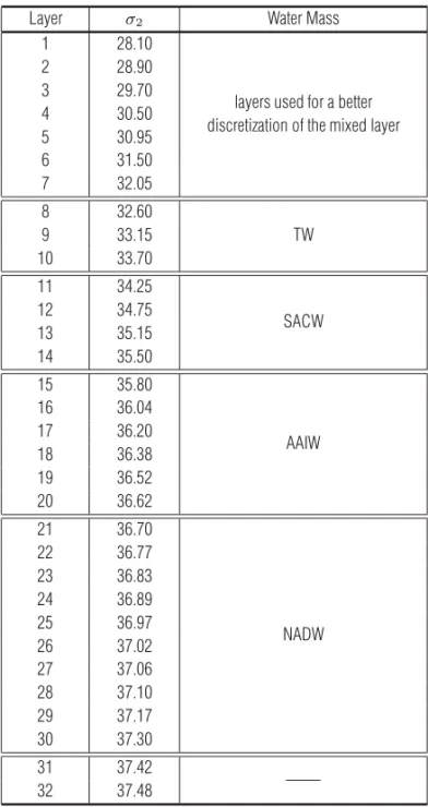
(Table 1). The simulation was initialized with the January clima-tology produced by the Generalized Digital Environment Model version 3.0 (GDEM3) (Carnes, 2009), which was developed by the Naval Oceanography Office (NAVOCEANO). The surface forc-ing was obtained from the Navy Operational Global Atmospheric Prediction System (NOGAPS) (HYCOM, 2007) and includes the wind and heat flux. The topography used in the model was derived from a quality controlled NRL DBDB2 bathymetry dataset (HY-COM, 2007). The model was integrated from 01/2003 to 04/2007. The monthly mean temperature and the salinity and velocity fields used in the present analysis were derived from model snapshots taken every three days from 2003 to 2005.
Table 1 – Vertical discretization in the layers ofσ2used in the HYCOM for the Western South Atlantic. Column 3 presents the water masses with a better repre-sentation by layer (TW – Tropical Water; SACW – South Atlantic Central Water; AAIW – Antarctic Intermediate Water; NADW – North Atlantic Deep Water).
Layer σ2 Water Mass
1 28.10
2 28.90
3 29.70
layers used for a better
4 30.50
discretization of the mixed layer
5 30.95 6 31.50 7 32.05 8 32.60 9 33.15 TW 10 33.70 11 34.25 12 34.75 SACW 13 35.15 14 35.50 15 35.80 16 36.04 17 36.20 AAIW 18 36.38 19 36.52 20 36.62 21 36.70 22 36.77 23 36.83 24 36.89 25 36.97 NADW 26 37.02 27 37.06 28 37.10 29 37.17 30 37.30 31 37.42 —— 32 37.48
To characterize the southwestern South Atlantic current sys-tem and to investigate SEC bifurcation, volume transports were computed within the density ranges corresponding to the main water masses in this region, for both the OCCAM and HYCOM. Several authors, such as Mamayev (1975), Reid (1989), Zemba (1991), Tomczak (1981), Memery et al. (2000), Ganachaud (2003) and You (2006), discuss different methods for characterizing the core and the vertical limits of the water masses. In the present work, these limits are based on the thermohaline indexes, in addition to the corresponding potential density surfaces pre-sented in the literature. For OCCAM,σθ = 25.70 (Mamayev, 1975; Stramma & England, 1999) separates the TW from SACW, σθ = 26.80 (Mamayev, 1975; Schott et al., 2005; Rodrigues
et al., 2007) separates the SACW from AAIW, andσθ = 27.53 (Stramma & England, 1999; Memery et al., 2000; Rodrigues et al., 2007) separates the AAIW from NADW. For the HYCOM, each water mass is represented by a group ofσ2isopycnal lay-ers, as listed in Table 1. The volume transports were calculated by integrating the velocities within the defined density ranges for the OCCAM and within the model layers for the HYCOM.
RESULTS AND DISCUSSION
In the present study, it is important to note the correct definition of the density limits that define each water mass. These limits are determined from the thermohaline indexes of each water mass, as presented in the methodology. Consequently, it is essential to es-timate how the vertical water mass structure is represented in the information under analysis. Thus, we estimated the mean fields of temperature and salinity for each simulation, where these values were compared with the climatology of the WOA05 (World Ocean Atlas 2005) (Locarnini et al., 2006; Antonov et al., 2006). It is worth noting that the present analyses are qualitative and that the simulations were validated in previous studies using the OCCAM (Lee & Coward, 2003; Marsh et al., 2005; Lee et al., 2007) and the HYCOM (Gabioux, 2008; Krelling, 2010).
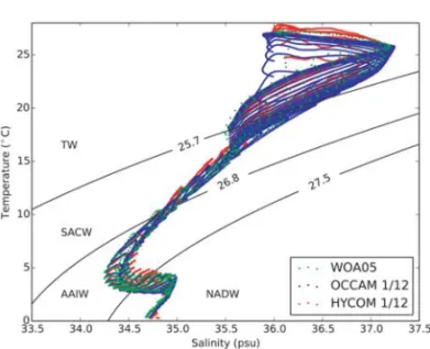
The thermohaline structure of the southwest South Atlantic is correctly represented in both cases (the OCCAM and HYCOM), and the main features of the TS diagrams compare well with the WOA05 climatology (Fig. 2). In both simulations, the TW is char-acterized by high values of potential temperature (θ >20◦C) and salinity (S>36), and the SACW by a typical linear θ-S rela-tionship (Sverdrup et al., 1942) between the thermohaline limits (6< θ <20◦C and 34.6<S<36.4). Both simulations represent the WOA05 data dispersion for central and intermediate waters (3< θ <6◦C and 34.2<S<36.4).
Figure 2 – Scatter diagrams of the annual means of the potential temperature
(θ) and salinity for the OCCAM 1/12◦(blue dot), HYCOM 1/12◦(red dot) and WOA05 1◦(green dot) at the longitude of 30◦W and within the latitude region from 1.5◦S to 35◦S.
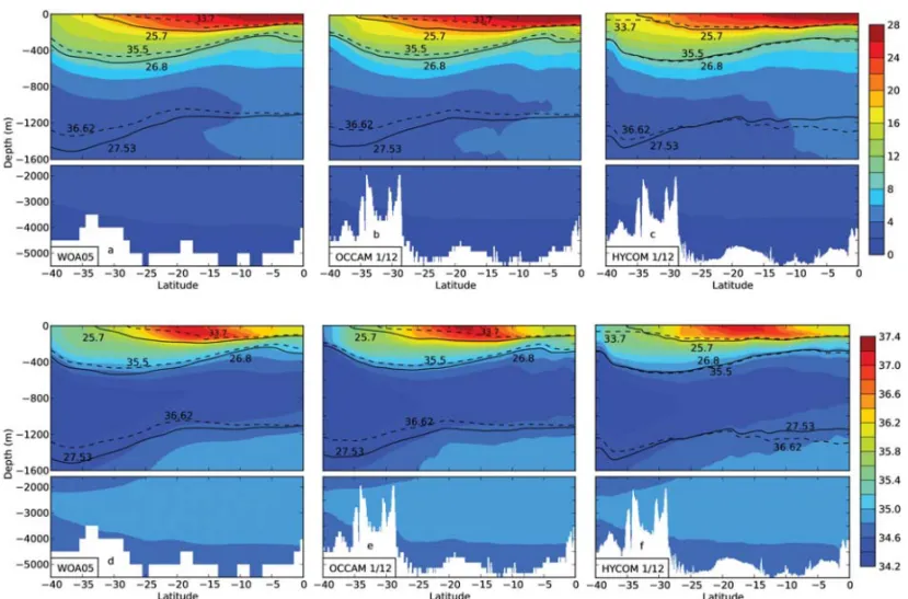
The vertical distribution of the water masses is also repre-sented in the two simulations. Figure 3 illustrates a meridional section of the temperature and salinity along 30◦W (between 40◦S and Equator) based on the OCCAM, HYCOM and WOA05. The locations in terms of depth of the water mass cores are prop-erly simulated. Near the surface, at locations close to tropical lat-itudes, the TW reaches temperature values of 28◦C and a salin-ity value of 37.5. At mid-depth, the SACW is represented by the temperature range of 6< θ <20◦C, with salinity values between 34.6 and 36, as found in the WOA05 dataset (Fig. 3a,d). The same features are presented in both high-resolution simulations (Fig. 3b,e,c,f). Beneath the SACW, the AAIW for WOA05 extends to∼1600 m of depth at 40◦S and grows shallower toward the north, reaching a depth of∼1000 m at the Equator (Fig. 3d). Below 1500 m of depth, the high salinity water of the NADW is found with a temperature below 4◦C and salinities higher than 34.6. With respect to the intermediate and deep waters, this pat-tern is also represented by the OCCAM and HYCOM simulations. Figure 3 also shows the isopycnalsσθandσ2, which define the water mass limits for the OCCAM (as well as WOA05) and HYCOM, respectively. It is interesting to note that despite several differences, the water mass limits computed withσθfor the OC-CAM andσ2for the HYCOM are generally in agreement over the domain. For all water masses, the difference between the base de-fined by the depth of a surface isopycnalσθor the depth of a layer σ2is less than∼ 15%.
Another approach used to assess the representativeness of the thermohaline fields simulated by the OCCAM and HYCOM is calculating the spatial distribution of the annual mean
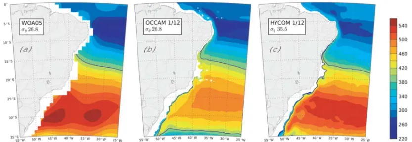
isopyc-nal layer depths, based on the limits presented in the respective methodology (Figs. 4, 5 and 6). The TW base (Fig. 4a-c) lies be-tween 60 and 200 m of depth. The TW base reaches deeper val-ues near 18◦S for the OCCAM, namely, at approximately 170 m (Fig. 4b), where this value also is close to that of the WOA05 dataset (Fig. 4a). A similar pattern is observed for the HYCOM, where the maximum depths (∼165 m) are located north of 28◦S (Fig. 4c). In the southern part of the BC region, between 25◦S and 35◦S, the TW base reaches depths of approximately 120 m in the HYCOM. The same feature is observed in the OCCAM until ∼30◦S (Fig. 4b).
In the case of the SACW/AAIW interface, both models agree with the climatology (Fig. 5). The SACW base shows a re-gion of maximum depth between 25◦S and 30◦S and a re-gion of minimum depth between 5◦S and 10◦S. The maximum depths simulated in the OCCAM (480 m, Fig. 5b) and HYCOM (∼ 500 m, Fig. 5c) are consistent with the observed values in WOA05 (Fig. 5a). In the northern part of the domain (beyond 15◦S), the depths reach values below 400 m. For the HYCOM the minimum depth is∼ 280 m, and for the OCCAM is ∼ 240 m. In intermediate waters, the main characteristics of the spatial pattern of the AAIW base, as observed in the climatology (Fig. 6a), are represented in the OCCAM (Fig. 6b). For both cases, the depth of the isopycnalσθ = 27.53 varies from 1000-1500 m, increasing toward higher latitudes. North of 24◦S, the depth of the isopycnal presents at shallower values, namely, 1200 m, in contrast south of 30◦S, it presents very deep levels of ap-proximately 1500 m. However, in the HYCOM, the AAIW base (Fig. 6c) presents a pattern of maximum depth at both the north and south boundaries (1300 m and 1400 m, respectively) and a minimum depth in the center of the domain at approximately 20◦S (∼ 1200 m). It is important to note that the differences be-tween the WOA05 and HYCOM AAIW base depths are less than 20% of the total thickness of the AAIW∼ 1000 m of depth, that is, differences as great as 200 m of depth appear only in a restricted region in the northern part of the domain.
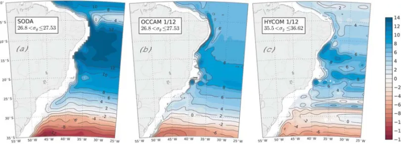
Once verified, the numerical results with respect to the thermohaline field define the limits between the densities of the water masses and are used to characterize the southwestern South Atlantic current system, as well as to investigate the SEC bifurcation. Accordingly, the annual, seasonal and monthly mean volume transport streamfunctions are computed for the defined density ranges (Figs. 7 to 10). In this part of the analysis, in ad-dition to the numerical results, other data-bases are also used, such as the SODA reanalysis from 1985 to 2004. The SODA ocean reanalysis was carried out based on the Parallel Ocean Program
Figure 3 – The meridional section at 30◦W of the annual mean temperature (upper panels) and salinity (lower panels) for the WOA05 dataset are given in (a) and (d), for the OCCAM 1/12◦in (b) and (e), and for the HYCOM 1/12◦in (c) and (f). The black solid lines indicate the isopycnal levels ofσθ25.7, 26.8 and 27.53, and the dashed lines indicate the isopycnal layer depths ofσ233.7, 35.5 and 36.62. The vertical axis forz ≤ 1600 m is expanded for visualization.
Figure 4 – The mean depth of the TW/SACW interface is represented by the isopycnalσθ25.7 for the WOA05 (a) and OCCAM 1/12◦(b) and byσ233.7 for the HYCOM 1/12◦(c). The bold line contour represents a depth of 100 m.
POP-1.4 model, which was 40 levels in the vertical direction and a 0.4× 0.25 degree displaced pole grid (Carton et al., 2000a,b). Flow bifurcations are defined by the position of the zero streamfunction near the coast. For the TW, SACW and AAIW, the presence of an approximately zonal flow indicates that the south
equatorial current corresponds to the northern branch of the sub-tropical gyre (Stramma & England, 1999).
At the TW level, the SEC bifurcation is located at∼15◦S in the HYCOM and SODA results. In contrast, the bifurcation ap-pears near 13◦S in the OCCAM, based on the annual means.
Figure 5 – The same as Figure 4 but for the SACW/AAIW interface (σθ= 26.8 and σ2= 35.5). The bold line contour represents a depth of 400 m.
Figure 6 – The same as Figure 4 but for the AAIW/NADW interface (σθ= 27.53 and σ2= 36.62). The bold line contour represents a depth of 1200 m.
Figure 7 – The mean volume transport of the TW, between the surface and the isopycnalσθ≤ 25.7 for SODA (a), OCCAM 1/12◦(b) and between the surface and the isopycnalσ2≤ 33.7 for HYCOM 1/12◦(c). The unit of transport is Sv. The contour interval is 1 Sv, with labels at every 2 Sv.
The seasonal variability of the SEC bifurcation for the TW level is summarized in Table 2 as monthly means for the OCCAM and HYCOM. In the OCCAM simulation, the SEC bifurcation reaches its northernmost position at 12◦S in December and its southern-most position at 16◦S in August. However, for the HYCOM, the northernmost position occurs in February and reaches 12.5◦S, while the southernmost position occurs at 17◦S during the aus-tral winter, which is in July. These results are consistent with the findings of Rodrigues et al. (2007) who used a reduced−gravity primitive equation for the OGCM and CTD data and found that the SEC bifurcation latitude reaches its northernmost position in November (∼13◦S in the uppermost 200 m) and its southernmost position in July (∼17◦S in the uppermost 200 m). The authors’ explanation for the seasonal variability of the bifurcation latitude in the upper thermocline is related primarily to variations in wind forcing based on the combined effect of local Ekman pumping and remotely forced Rossby waves.
South of the bifurcation latitude, a part of the SEC creates a southward flowing limb, which gives rise to the BC. At 25◦S, the TW transport carried by the BC is 2 Sv for the OCCAM and SODA (Fig. 7b, a) and is 4 Sv for the HYCOM (Fig. 7c). North of the bi-furcation latitude, the northern branch of the SEC feeds the NBC. Silveira et al. (1994) estimated the geostrophic transport of the NBC to be 6.5 Sv (the section located at 5◦S between 34◦30’W – 32◦00’W from the surface to 100 m of depth). At the same lat-itude, the TW transport is 9 Sv for the OCCAM simulation, 6 Sv for the HYCOM and 10 Sv for SODA.
Below the TW, at the SACW level, the SEC bifurcation is shifted southward and is located at approximately 22◦S for both high-resolution simulations (Fig. 8b and c) and at 23◦S for SODA (Fig. 8a). These values are closer to the SEC bifurcation latitude calculated by Stramma & England (1999) (∼20◦S, from approx-imately 100 m to 500 m) and Rodrigues et al. (2007) (∼21◦S at 400 m). The southernmost position of the SEC bifurcation occurs in December (21◦S for the OCCAM) and in January (21◦S for the HYCOM).
At the SEC bifurcation, a part of the SACW flows northward with the North Brazil Undercurrent (NBUC), while another part flows southward with the BC. At latitudes north of 15◦S, the NBUC merges with the surface flow, forming the NBC system, which ap-pears as an intensified northwestward flow as it moves beyond the Equator. At 5◦S, the SACW transport carried by the NBUC is es-timated as 10 Sv for the OCCAM simulation and SODA (Fig. 8b and a) and as 9 Sv for the HYCOM (Fig. 8c).
In intermediate waters, the SEC bifurcation is located at ap-proximately 30◦S for the OCCAM simulation (Fig. 9b) and at
28◦S for SODA and the HYCOM (Fig. 9a,c). For the mean flow field of the AAIW, Stramma & England (1999), Boebel et al. (1999) and Schmid & Garzoli (2009) represent the northern limb of the subtropical gyre reaching the Brazilian continent at approximately 28◦S. Rodrigues et al. (2007) found that the annual mean SEC bi-furcation latitude, which occurs at 900 m, is approximately 26◦S. In the OCCAM simulation, the SEC bifurcation presents a sea-sonal shift from 35◦S in June and 28◦S in December. In the HYCOM, the seasonal variability exhibits its southernmost po-sition in July at 32.5◦S, while the northernmost position appears in November at 25◦S (Table 2). The seasonal variability of the SEC bifurcation simulated by Rodrigues et al. (2007), at 900 m, presents the southernmost position of the bifurcation at 27◦S in July, while in October, the northern position occurs at 26◦S. At this level (the northernmost position of the bifurcation), the AAIW is carried northward by the IWBC. The northward flow was es-timated from direct observations for April 1983 along 22-23◦S by Silveira et al. (2004) to be 3.6 Sv. The values for the OC-CAM and HYCOM are 4 Sv near the same region and 6 Sv for SODA. Schmid & Garzoli (2009) estimated a mean transport of the IWBC between 28◦S and 6◦S of 2.8 Sv with maximum values of∼ 10 Sv near 20◦S. The simulation results from the OCCAM, HYCOM and SODA analyses present transport values near this region that are approximately∼ 8 Sv.
The latitudinal variation of the SEC bifurcation with depth is consistent with the values found in the literature. Wienders et al. (2000) estimated the SEC bifurcation from hydrographic data obtained in January-March 1994 and found that the bifurca-tion ranges downward from approximately 14◦S at the surface to 28◦S at a depth of 600 m. Based on annual mean CTD observation data, Rodrigues et al. (2007) found that the bifurcation occurs at 21◦S at a depth of 400 m, representing a southward displacement of 7 degrees from its surface value (14◦S).
A relatively intense and well organized flow carries the NADW southward along the Brazilian continental margin as a Deep West-ern Boundary Current (DWBC), and this pattWest-ern is well repre-sented in all simulations, as well as in SODA (Fig. 10). This flow presents an eastward turning between 20◦S and 22.5◦S that is related to the presence of the Vit´oria-Trindade Ridge, which is a bathymetric obstacle that resides perpendicular to the continental slope at 20◦S-21◦S (Fig. 1). The eastward turning was also ob-served by Memery et al. (2000) at the A17 WOCE line. The NADW transport is estimated at 11◦S as 21 Sv in SODA and 18 Sv in the OCCAM and HYCOM simulations and at 19◦S as 18 Sv in SODA, 15 Sv in the OCCAM and 12 Sv in the HYCOM. These values un-derestimate the NADW transport described in Ganachaud (2003).
Table 2 – The seasonal variability of the SEC bifurcation for the OCCAM 1/12◦and the HYCOM 1/12◦. OCCAM 1/12◦ HYCOM 1/12◦
Month
TW SACW AAIW TW SACW AAIW
January 13◦S 21.5◦S 30◦S 13◦S 21◦S 27.5◦S February 13◦S 21.5◦S 30◦S 12.5◦S 22◦S 27.5◦S March 14◦S 22◦S 31◦S 14.5◦S 22.5◦S 30◦S April 14◦S 23◦S 32◦S 15◦S 22.5◦S 27◦S May 15◦S 24◦S 32◦S 15◦S 22◦S 27.5◦S June 15.5◦S 25◦S 35◦S 15.5◦S 23◦S 30◦S July 16◦S 24◦S 34◦S 17◦S 23◦S 32.5◦S August 16◦S 23◦S 32◦S 15.5◦S 22◦S 26◦S September 14.5◦S 22◦S 32◦S 15◦S 21.5◦S 26◦S October 13◦S 22◦S 31◦S 15◦S 22◦S 25.5◦S November 12.5◦S 22◦S 29◦S 14.5◦S 22◦S 25◦S December 12◦S 21◦S 28◦S 14.5◦S 22◦S 26◦S
Figure 8 – The same as Figure 7 but for the SACW, between the isopycnal intervals of 25.7< σθ≤ 26.8 for (a), (b); and 33.7 < σ2≤ 35.5 for (c).
Figure 10 – The same as Figure 7 but for the NADW, between the isopycnal intervals ofσθ> 27.53 and the bottom for (a), (b) and between the isopycnals σ2> 36.62
and the bottom (c). The contour interval is 3 Sv.
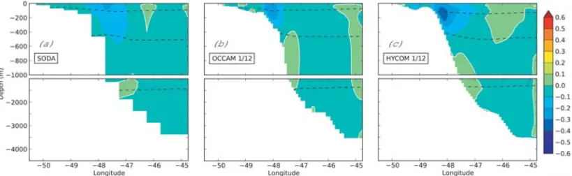
Figure 11 – The mean meridional velocity (m s−1) at the latitude of 5◦S for SODA (a), OCCAM 1/12◦(b), and HYCOM 1/12◦(c). The white contour represents the zero velocity, while values higher than 0.6 are shown as dotted contours. The black dashed lines indicate the isopycnal levels ofσθ25.7, 26.8 and 27.53 in (a), (b) andσ233.7, 35.5 and 36.62 in (c). The vertical axis forz ≤ 1000 m is expanded for better visualization. The location of the section is indicated in Figure 1. Positive values for velocity and transport indicate a northward flow.
According to the author, the NADW transport values calculated during the WOCE period (1985-1996) for sections at 11◦S (A8) and 19◦S (A9) are 23 Sv at both lines.
To complement the analysis of the southwestern Atlantic re-gion, we examine the annual mean vertical velocity structure of the WBC in conjunction with the volume transport for each water mass. This computation is performed for zonal sections at key lo-cations along the western boundary. The location of each section is shown in Figure 1, and the transports for annual and seasonal are summarized in Tables 3, 4 and 5 for the OCCAM, HYCOM and SODA analyses, respectively.
At 5◦S, in all simulations, although less apparent for SODA, the WBC system presents a bimodal structure with a northward flow in the first 1300 m of depth, identified as the NBUC, and a southward flow underneath, known as the DWBC (Fig. 11). The NBUC shows a significant core of annual mean meridional
veloci-ties as large as 0.6 m s−1from∼50 m to 400 m of depth, reaching maximum values of 1.12± 0.07 m s−1, 0.82± 0.15 m s−1and 0.93± 0.10 m s−1for the OCCAM (Fig. 11b), SODA (Fig. 11a) and HYCOM (Fig. 11c) analyses, respectively. These values are slightly higher than the velocity of 0.8 m s−1calculated by Schott et al. (2005). Below the NBUC, between 1200 and 3300 m of depth, the DWBC presents maximum meridional velocities of 0.30 ± 0.05 m s−1 for the OCCAM and 0.20± 0.04 m s−1for the
HYCOM. These values also are in agreement with the velocity of 0.2 m s−1calculated by Schott et al. (2005).
At this section and in the uppermost 1000 m of depth, the NBUC transport is associated with the TW, SACW and AAIW (Fig. 11). The NBUC mean annual transport calculated as a sum-mation of the TW, SACW and AAIW transports is 30.2 Sv for the OCCAM (Table 3), 22.4 Sv for the HYCOM (Table 4) and 33.8 Sv for SODA (Table 5). At the same latitude, Schott et al. (2005)
estimated a mean transport of 26.5± 3.7 Sv above the σ1 = 32.15 isopycnal (∼1000 m depth). Below the AAIW layer, the NADW transport values calculated for the OCCAM, HYCOM and SODA are 17.8± 4.1 Sv, 16.1 ± 3.5 Sv and 18.0 ± 3.5 Sv, re-spectively. Schott et al. (2005) found a mean southward DWBC transport of 25.5± 8.3 Sv for nine measured sections during 1990-2004, ranging betweenσ1= 32.15 and σ4= 45.90 west of 33.5◦W. In relation to the seasonal transport variation of the NBUC, the maximum values are observed in winter for all of the analyzed results (Tables 3, 4 and 5). In this case, the DWBC trans-port maximum arises during summer.
At 13◦S (Fig. 12), the main circulation feature is the IWBC, which is located in the upper 1300 m of depth. Legeais et al. (2013) present a IWBC mean velocity at 15◦S of∼ 0.08 m s−1 that increases to 0.2 m s−1 at 10◦S with a maximum value of 0.7 m s−1. In both high-resolution simulations, the IWBC core is confined between 200-800 m of depth (Fig. 12b, c). The maximum velocities are 0.42 ± 0.10 m s−1 for the OCCAM, 0.44± 0.09 m s−1 for the HYCOM and 0.29± 0.08 m s−1 for SODA. In this section, we found the origin of the BC near the surface (∼ the first 50 m of depth) for in the OCCAM simula-tion, although this was not observed for either the HYCOM or SODA analysis. This difference is a result of the bifurcations in the HYCOM and SODA analyses south of 13◦S (at approxi-mately 15◦S – Fig. 7a, c).
Below the IWBC appears the DWBC, which transports the NADW. This boundary current presents maximum velocities of 0.19± 0.05 m s−1for the OCCAM, 0.10± 0.04 m s−1for the HYCOM and 0.07± 0.02 m s−1for SODA (Fig. 12).
In terms of transport, the IWBC appears as a boundary cur-rent constituted mainly of the SACW and the AAIW, transporting northward flows of∼20 Sv, ∼23 Sv and ∼24 Sv in the OCCAM, HYCOM and SODA analyses, respectively. In this same section, the southern flow of the NADW is estimated to be∼26 Sv for the OCCAM,∼31 Sv for the HYCOM and ∼24 Sv for SODA. Here, the maximum values of the SACW, AAIW and NADW trans-ports are observed in winter based on the OCCAM, HYCOM and SODA analyses (Tables 3, 4 and 5). At 11◦S, Schott et al. (2005) observed a northward NBUC maximum in July and minimum in October-November. For NADW transport at the same latitude, the authors observed maximum values in November and minimum values in July.
At 22◦S, the TW and a fraction of the SACW are transported southward by the BC, which resides in the upper levels (Fig. 13). West of 39.3◦W, the BC appears well developed in all simula-tions and SODA (Fig. 13a-c), extending through the upper 300 m
of depth. The maximum annual meridional velocities found for the BC are 0.55 m± 0.14 s−1, 0.54± 0.15 m s−1and 0.43 ± 0.11 m s−1 for the OCCAM, HYCOM and SODA analyses,
respectively. Near this latitude, in a transect at 22.75◦S, Oliveira et al. (2009) found the BC velocity to be 0.39± 0.23 m s−1using surface drifter data.
Below 300 m of depth, part of the SACW is carried north-ward. This occurs due to shifting of the SEC bifurcation with depth, which is located approximately at this level at 22◦S (Fig. 8). The northward SACW and AAIW flows depict a IWBC with a defined core that is confined between 400 and 1000 m, the associated velocities are 0.26± 0.09 m s−1for the OCCAM, 0.54± 0.15 m s−1for the HYCOM and 0.43± 0.11 m s−1for SODA. At this latitude, for all simulations, the DWBC core presents maximum velocities as great as 0.1 m s−1and is located at 38.5◦W between the depths of 2000 m and 2500 m. The DWBC maximum velocity for the OCCAM is 0.17± 0.04, for the HYCOM is 0.12± 0.04 m s−1and for SODA is 0.05± 0.02 m s−1.
Based on observations that the mean transport value of the BC is 8.6± 4.1 Sv at 24◦S and 19.4± 4.3 Sv at 35◦S, Garzoli et al. (2013) found that the BC increases toward the south. From a velocity cross-section developed during the Transport of the Brazil Current Experiment (TRANSCOBRA, 1982–1984), carried out at 22◦–23◦S, Silveira et al. (2004) estimated a BC transport of 5.6± 1.4 Sv and a IWBC transport of 3.6 ± 0.8 Sv. To compare these values, we computed the BC and the IWBC transport cores in the section at 22◦S, located between land and the longitude of 39.3◦W, and we obtained BC transports of 2.99 Sv and 3.07 Sv for the OCCAM and HYCOM, respectively. For the IWBC, we found transports of 5.70 Sv and 9.20 Sv for the OCCAM and HYCOM (not shown). Below the IWBC, the NADW transports were com-puted as∼12 Sv, 11 Sv and 20 Sv for the OCCAM, HYCOM and SODA analyses, respectively. In this section, the seasonal cycles for the BC, IWBC and DWBC are less clear than in the previous sections.
Finally, in the southern part of our domain, at 30◦S, the BC grows deeper (reaching approximately 400-500 m of depth in all simulations and SODA, as shown in Fig. 14) because the bifur-cation of the intermediate flow occurs near this latitude (Fig. 9). The BC maximum velocities for the OCCAM, HYCOM and SODA analyses are 0.34± 0.07 m s−1, 0.33± 0.15 m s−1and 0.23± 0.08 m s−1, respectively. Unlike the BC, the IWBC in this section is slightly less intense for SODA than for the other simulations. In the section at 30◦S, the seasonal cycles of the BC, IWBC and DWBC transport also are less evident.
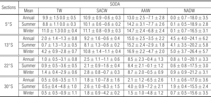
Table 3 – The transport (Sv) for each water mass of the OCCAM 1/12◦at the analyzed sections for the annual mean, summer and winter. OCCAM 1/12◦
Sections
Mean TW SACW AAIW NADW
Annual 8.9± 1.7 –0.1 ± 0.3 11.0± 1.0 –0.5 ± 0.5 10.3± 2.7 –3.8 ± 2.6 3.4± 1.6 –17.8 ± 4.1 5◦S Summer 8.2± 1.6 –0.0 ± 0.1 10.4± 0.9 –0.4 ± 0.4 9.5± 2.0 –5.1 ± 2.8 2.3± 1.1 –20.6 ± 2.9 Winter 8.8± 1.2 –0.3 ± 0.4 11.5± 0.9 –0.5 ± 0.5 11.0± 2.8 –2.1 ± 1.5 3.8± 1.6 –14.2 ± 3.6 Annual 3.0± 1.4 –1.3 ± 1.0 7.6± 1.6 –0.3 ± 0.4 12.3± 2.6 –4.1 ± 2.7 9.8± 7.0 –26.5 ± 7.6 13◦S Summer 2.2± 1.0 –2.2 ± 1.2 6.4± 1.1 –0.4 ± 0.6 11.0± 2.6 –4.1 ± 3.0 7.7± 6.1 –23.2 ± 5.9 Winter 4.1± 1.1 –0.5 ± 0.5 8.9± 1.3 –0.2 ± 0.3 13.7± 2.0 –3.8 ± 2.6 11.3± 8.6 –28.4 ± 9.3 Annual 1.1± 0.8 –3.0 ± 0.8 3.3± 1.3 –2.2 ± 1.1 10.9± 3.0 –3.5 ± 2.9 2.9± 2.0 –12.3 ± 1.5 22◦S Summer 1.2± 0.8 –3.2 ± 0.7 3.3± 1.3 –2.4 ± 1.2 10.9± 3.3 –3.5 ± 3.4 2.9± 1.8 –11.1 ± 2.6 Winter 0.8± 0.6 –2.5 ± 0.8 2.9± 1.1 –1.8 ± 0.9 10.2± 2.9 –3.5 ± 2.5 2.2± 2.0 –12.4 ± 2.1 Annual 0.8± 0.8 –2.9 ± 1.2 1.8± 1.3 –5.5 ± 1.5 3.2± 2.1 –4.8 ± 2.2 0.6± 0.5 –10.9 ± 2.7 30◦S Summer 0.8± 0.9 –3.5 ± 1.1 1.8± 1.4 –6.1 ± 1.4 2.7± 2.2 –5.0 ± 2.4 0.6± 0.6 –10.5 ± 2.6 Winter 0.9± 0.9 –2.5 ± 1.3 1.7± 1.1 –4.9 ± 1.4 3.7± 2.1 –4.9 ± 1.9 0.5± 0.4 –11.5 ± 2.4 Table 4 – The transport (Sv) for each water mass of the HYCOM 1/12◦at the analyzed sections for the annual mean, summer and winter.
HYCOM 1/12◦
Sections
Mean TW SACW AAIW NADW
Annual 5.9± 0.9 –0.8 ± 0.5 9.4± 0.4 –0.7 ± 0.2 7.1± 1.6 –3.9 ± 2.1 2.8± 0.8 –16.1 ± 3.5 5◦S Summer 4.7± 1.1 –0.8 ± 0.7 9.0± 0.6 –0.7 ± 0.1 6.4± 1.4 –6.2 ± 1.4 2.1± 0.5 –20.3 ± 1.6 Winter 5.7± 0.2 –1.3 ± 0.4 9.6± 0.6 –0.9 ± 0.1 7.9± 1.2 –2.1 ± 1.0 3.7± 0.8 –13.1 ± 1.8 Annual 4.0± 1.2 –2.1 ± 0.8 8.7± 0.8 –0.7 ± 0.4 14.1± 1.2 –6.1 ± 2.7 11.2± 3.4 –31.2 ± 4.8 13◦S Summer 2.3± 0.2 –2.1 ± 0.8 7.4± 0.4 –0.3 ± 0.1 12.5± 0.7 –4.6 ± 2.0 8.7± 2.6 –29.8 ± 3.4 Winter 5.1± 0.6 –2.5 ± 1.2 9.8± 0.1 –0.7 ± 0.3 14.7± 0.6 –5.0 ± 1.9 11.3± 5.6 –35.5 ± 1.1 Annual 1.1± 0.4 –3.4 ± 0.5 2.6± 0.7 –2.4 ± 0.5 9.1± 1.4 –3.1 ± 1.0 4.2± 1.1 –11.0 ± 1.2 22◦S Summer 0.9± 0.1 –3.7 ± 0.5 1.9± 0.1 –2.4 ± 0.5 7.7± 1.6 –3.6 ± 0.5 3.2± 0.9 –10.5 ± 0.9 Winter 1.4± 0.3 –3.0 ± 0.3 3.7± 0.6 –2.2 ± 0.4 10.6± 0.5 –2.9 ± 0.8 4.0± 0.7 –11.5 ± 0.9 Annual 2.4± 0.8 –6.8 ± 1.1 4.2± 1.5 –10.3 ± 1.2 4.8± 1.4 –7.5 ± 1.1 2.6± 0.7 –12.0 ± 2.1 30◦S Summer 1.7± 0.7 –8.2 ± 0.8 2.8± 0.9 –11.1 ± 0.8 3.1± 0.4 –8.8 ± 0.7 2.3± 0.6 –11.1 ± 1.3 Winter 3.2± 0.7 –6.1 ± 0.2 4.6± 1.4 –9.8 ± 0.6 6.4± 0.9 –7.4 ± 0.6 3.5± 0.3 –14.5 ± 1.1 Table 5 – The transport (Sv) for each water mass of SODA at the analyzed sections for the annual mean, summer and winter.
SODA Sections
Mean TW SACW AAIW NADW
Annual 9.9± 1.5 0.0 ± 0.5 10.9± 0.9 –0.6 ± 0.3 13.0± 2.5 –7.1 ± 2.8 0.0± 0.7 –18.0 ± 3.5 5◦S Summer 8.8± 1.1 0.0 ± 0.3 10.1± 0.6 –0.6 ± 0.2 14.2± 3.1 –7.7 ± 2.6 0.1± 0.5 –18.9 ± 2.8 Winter 11.0± 1.3 0.0 ± 0.4 11.1± 0.8 –0.9 ± 0.3 14.7± 2.4 –6.8 ± 2.4 0.1± 0.7 –16.5 ± 3.1 Annual 2.0± 1.4 –1.3 ± 0.8 9.2± 1.6 –0.6 ± 0.4 15.0± 2.5 –3.5 ± 2.2 4.5± 4.0 –24.1 ± 6.2 13◦S Summer 0.7± 1.3 –1.3 ± 0.5 8.1± 1.3 –0.6 ± 0.2 15.2± 2.4 –2.9 ± 1.8 4.1± 3.5 –20.2 ± 5.8 Winter 4.2± 0.9 –2.8 ± 0.7 10.8± 1.4 –1.1 ± 0.4 16.9± 2.2 –4.7 ± 2.0 5.0± 3.7 –26.4 ± 5.7 Annual 1.0± 0.5 –3.1 ± 0.8 2.5± 1.1 –1.1 ± 0.6 8.5± 2.3 –0.4 ± 1.3 0.8± 1.0 –20.1 ± 3.3 22◦S Summer 0.9± 0.5 –3.6 ± 0.5 2.1± 0.9 –1.6 ± 0.4 8.4± 2.1 –0.1 ± 1.2 0.6± 0.8 –17.5 ± 3.0 Winter 1.4± 0.4 –2.9 ± 0.6 2.8± 0.8 –0.7 ± 0.3 8.7± 2.0 –0.5 ± 0.9 0.9± 0.9 –21.2 ± 3.1 Annual 0.5± 0.6 –3.5 ± 1.1 1.8± 1.0 –7.8 ± 1.6 2.1± 1.2 –6.5 ± 2.6 1.1± 0.6 –17.0 ± 3.6 30◦S Summer 0.5± 0.4 –4.8 ± 1.0 2.6± 1.0 –8.3 ± 1.5 4.0± 0.9 –7.2 ± 2.1 1.9± 0.4 –15.5 ± 2.4 Winter 0.5± 0.5 –0.9 ± 1.1 1.8± 0.9 –4.2 ± 0.2 1.5± 1.0 –4.8 ± 1.2 0.7± 0.5 –15.6 ± 3.5
Figure 12 – The same as Figure 11, but at the latitude of 13◦S.
Figure 13 – The same as Figure 11, but at the latitude of 22◦S.
In this section, the southward NADW transport simulated by the OCCAM is 10.9± 2.7 Sv and gives values of 12.0 ± 2.1 Sv for the HYCOM and 17.0± 3.6 Sv for SODA (Tables 3, 4 and 5). In all simulations and for SODA, the NADW transport values underestimate the value of 23± 3 Sv calculated by Ganachaud (2003), which aggregates the return of the Antarctic Bottom Water and the AAIW as they progress southward.
CONCLUSIONS
The results of two eddy resolving (1/12◦) OGCMs were used to investigate the flow bifurcations of the Western Boundary Current system (WBC) and the water masses of the Western South Atlantic Ocean. Particular attention was given to the latitude of bifurcation of the currents feeding into the WBC system, with a focus on the flow associated with the different water masses. Considering that observations of the South Atlantic WBC system are sparse, in ad-dition to the fact that previous knowledge regarding the WBC bi-furcation is based on limited data observations and coarse numer-ical simulations, these two independent simulations with realistic high-resolution OGCMs offer an interesting source of additional information.
The numerical models used were the OCCAM in z-coor-dinates and the HYCOM in hybrid-coorz-coor-dinates. Modeling com-parisons have long been performed, for example, the DYNAMO (Willebrand et al., 2001) and the DAM´EE-NAB (Chassignet et al., 2000) projects, with a predominant focus on model performance. The DYNAMO project, for example, investigated the role of differ-ent vertical model discretizations using the GFDL-MOM (level), MICOM (isopycnal) and SPEM (sigma). The project contributed to our understanding of the circulation in the North Atlantic Ocean and showed that verticalz-level coordinates affect the integrity of water masses as a result of the excessive diapycnal mixing that is induced by the numerical algorithms (Willebrand et al., 2001).
In the present work, the water masses were separated by ther-mohaline index. Theσθlevels were defined for the OCCAM simu-lation, andσ2layers were considered for the HYCOM. The current transports were calculated for these isopycnal ranges. Overall, the bimodal system of the WBC in the South Atlantic Ocean, which presents a southward flow in the upper layers and a northward flow in the intermediate layers (Stramma & England, 1999; Sil-veira et al., 2000), was captured by these high-resolution simula-tions, with respect to both the vertical structure of the flow and the intensity of the currents. The location of the SEC bifurcation near the coast (within the first 1500 m of depth) shifts southward with increasing depth, as previously described by Stramma & England (1999); Reid (1989); Rodrigues et al. (2007). At the TW level, the
SEC bifurcates at approximately 13◦S and 15◦S in the OCCAM and HYCOM, respectively. At the SACW level, the bifurcation is located at approximately 22◦S in both high-resolution simula-tions. At intermediate levels, the southern limb of the SEC reaches the Brazilian continent at approximately 28◦S in the HYCOM (in agreement with Stramma & England (1999); Boebel et al. (1999); Schmid & Garzoli (2009)), and at 30◦S in the OCCAM simulation. The models indicate that there is significant seasonal vari-ation in the latitudes of the bifurcvari-ations. At the TW level, the SEC reaches its most northerly position at 12◦S in December for the OCCAM simulation and at 12.5◦S in February for the HYCOM. The southerly position of the bifurcation was found at 16◦S in August for the OCCAM and at 17◦S in July for the HY-COM. At the SACW level, the most northerly position is located at 21◦S for both high-resolution simulations (in December for the OCCAM and January for the HYCOM), and the southerly po-sitions are located at 25◦S and 23◦S in June for the OCCAM and HYCOM, respectively. Finally, at intermediate levels, the most northerly/southerly positions occur in November for the HYCOM and in December for the OCCAM, at 25◦S and 28◦S, respec-tively, and at 32.5◦S in July for the HYCOM and 35◦S in June for the OCCAM.
The present study indicates that bifurcations at the latitudes suggested by previous studies are a robust feature of this cur-rent system. These two realistic and independent high-resolution global simulations add confidence to the values presented in the literature regarding the flow bifurcations at the Brazilian coast.
ACKNOWLEDGMENTS
The National Oceanography Centre, Southampton (NOCS) kindly provided the OCCAM results, while the HYCOM outputs were provided by the Center for Ocean-Atmospheric Prediction Stud-ies (COAPS). This research was supported by the Oceanographic Modeling and Observation Network (REMO), funded with research grants from Petrobras and approved by the Brazilian Petroleum Agency (Agˆencia Nacional do Petr´oleo, G´as Natural e Biocom-bust´ıveis – ANP).
REFERENCES
ANTONOV JI, LOCARNINI RA, BOYER TP, MISHONOV AV & GARCIA HE. 2006. World Ocean Atlas 2005 Volume 2: Salinity S. Levitus. 182 pp., Ed. NOAA Atlas NESDIS 62, U.S Gov. Printing Office, Washington, D.C. BLECK R, HALLIWELL GRJ, WALLCRAFT AJ, CARROLL S, KELLY K & RUSHING K. 2002. HYCOM User’s Manual Details of the numerical code. online Manual Version 2.0.01, University of Miami, USA. 211 pp.
BOEBEL O, SCHMID C & ZENK W. 1997. Flow and recirculation of Antarctic Intermediate Water across the Rio Grande Rise. J. Geophys. Res., 102: 20967–20986.
BOEBEL O, DAVIS R, OLLITRAUT M, PETERSON R, RICHARD P, SCHMID C & ZENK W. 1999. The Intermediate Depth Circulation of the Western South Atlantic. Geophys. Res. Lett., 26: 3329–3332.
BRYAN K. 1969. A numerical method for the study of the circulation of the world ocean. J. Comput. Phys., 4: 347–376.
CARNES MR. 2009. Description and evaluation of GDEM-V3.0. Tech. Rep. NRL/MR/7330-09-9165, Naval Research Laboratory, Stennis Space Center, MS, USA.
CARTON J, CHEPURIN G, CAO X & GIESE B. 2000a. A simple ocean data assimilation analysis of the global upper ocean 1950-95. part 1: Methodology. J. Phys. Oceanogr., 30: 294–309.
CARTON J, CHEPURIN G, CAO X & GIESE B. 2000b. A simple ocean data assimilation analysis of the global upper ocean 1950-95. part 2: Results. J. Phys. Oceanogr., 30: 311–326.
CHASSIGNET EP, ARANGO H, DIETRICH D, EZER T, GHIL M, HAIDVO-GEL DB, MA CC, MEHRA A, PAIVA AM & SIRKES Z. 2000. DAMEENAB: the base experiments. Dyn. Atmos. Ocean, 32: 155–183.
CIRANO M, MATA MM, CAMPOS EJD & DEIR ´O NFR. 2006. A Circulac¸˜ao Oceˆanica de Larga-Escala na Regi˜ao Oeste do Atlˆantico Sul com base no modelo de Circulac¸˜ao Global OCCAM. Brazilian Journal of Geophysics, 24(2): 209–230.
COWARD AC & CUEVAS BA. 2005. The OCCAM 66 level model: physics, initial conditions and external forcing. Southampton OceanographyCen-tre – Technical Report, 99: 1–58.
COX M. 1984. A primitive equation 3-dimensional model of the ocean. Geophysical Fluid Dynamics Laboratory Technical Report, 1: 1–143. GABIOUX M. 2008. Estudo Num´erico dos Meandros e V´ortices da Cor-rente do Brasil entre 22◦S e 30◦S. Ph.D. thesis, Programa de Engenharia Oceˆanica – COPPE/UFRJ, Rio de Janeiro. 142 pp.
GANACHAUD A. 2003. Large-scale mass transport, water mass forma-tion, and diffusivities estimated from World Ocean Circulation Experiment WOCE hydrografic data. J. Geophys. Res., 108: 3213, doi: 10.1029/ 2002JC001,1565.
GARZOLI SL, BARINGER MO, DONG S, PEREZ RC & YAO Q. 2013. South Atlantic meridional fluxes. Deep Sea Res. I, 71: 21–32.
GOURETSKIVV & JANKE K. 1996. A new hydrografic data set for the south pacific: synthesis of WOCE and historical data. Tech. Rep., WOCE Report No. 143/96.
HOGG NG & THURNHERR AM. 2005. A zonal pathway for NADW in the South Atlantic. J. Oceanography, 61: 493–507.
HYCOM. Hybrid Coordinate Ocean Model. 2007. Non-Assim-ilative Global Simulation (01/2003 to 04/2007). Available on: <http://hycom.coaps.fsu.edu/data/glb-simulation>. Access on: March 1, 2010.
KALNAY E, KANAMITSU M, KISTLER R, COLLINS W, DEAVEN D, GANDIN L, IREDELL M, SAHA S, WHITE G, WOOLLEN J, ZHU Y, CHEL-LIAH M, EBISUZAKI W, HIGGINS W, JANOWIAK J, MO KC, ROPELEWSKI C, WANG J, LEETMAA A, REYNOLDS R, JENNE R & JOSEPH D. 1996. The NCEP/NCAR 40-year reanalysis project. Bull. Am. Meteorol. Soc., 77: 437–471.
KRELLING APM. 2010. A Estrutura Vertical dos V´ortices da Corrente Norte do Brasil. Master dissertation, Programa de Engenharia Oceˆanica – COPPE/UFRJ, Rio de Janeiro, RJ, 60 pp.
LARGE WG, DANABASOGLU G, DONEY SC & McWILLIAMS JC. 1997. Sensitivity to surface forcing and boundary layer mixing in a global ocean model: Annual-Mean Climatology. J. Phys. Oceanogr., 27: 2418–2447. LEE MM & COWARD A. 2003. Eddy mass transport for the Southern Ocean in an eddy-permitting global ocean model. Ocean Model, 5: 249– 266.
LEE MM, NURSER AJG, COWARD AC & CUEVAS BA. 2007. Eddy ad-vective and diffusive transports of heat and salt in the Southern Ocean. J. Phys. Oceanogr., 37: 1376–1393.
LEGEAIS JF, OLLITRAULT M & ARHAN M. 2013. Lagrangian Observa-tions in the Intermediate Western Boundary Current of the South Atlantic. Deep Sea Res. II, 85: 109–126.
LOCARNINI RA, MISHONOV AV, ANTONOV JI, BOYER TP & GARCIA HE. 2006. World Ocean Atlas 2005 Volume 1: Temperature S. Levitus. 182 pp., Ed. NOAA Atlas NESDIS 61, U.S Gov. Printing Office, Washing-ton, D.C.
MAMAYEV OI. 1975. Temperature-salinity analysis of the world ocean waters. Elsevier Scientific Publ., Amsterdam. 374 pp.
MANO MF, PAIVA AM, TORRES Jr AR & COUTINHO ALGA. 2009. En-ergy Flux to a Cyclonic Eddy off Cabo Frio, Brazil. J. Phys. Oceanogr., 39: 2999–3010.
MARSH R, JOSEY SA, NURSER AJG, CUEVAS BA & COWARD AC. 2005. Water mass transformation in the North Atlantic over 1985-2002 simulated in an eddy-permitting model. Ocean Science, 1: 127–144. MEMERY L, ARHAN M, ALVAREZ-SALGADO XA, MESSIAS MJ, MERCIER H, CASTRO CG & RIOS AF. 2000. The water masses along the western boundary of the south and equatorial Atlantic. Prog. Oceanogr., 47: 69–98.
MIRANDA LB. 1985. Forma da correlac¸˜ao T-S de massas de ´agua das regi˜oes costeira e oceˆanica entre o Cabo de S˜ao Tom´e (RJ) e a Ilha de S˜ao Sebasti˜ao (SP), Brasil. Bol. Inst. Oceanogr. S˜ao Paulo, 33: 105– 119.
MULLER T, IKEDA Y, ZANGENBERG N & NONATO L. 1998. Direct mea-surements of the western boundary currents off Brazil between 20◦S and 28◦S. J. Geophys. Res., 103: 5429–5437.
OLIVEIRA LR, PIOLA AR, MATA MM & SOARES ID. 2009. Brazil Cur-rent surface circulation and energetics observed from drifting buoys. J. Geophys. Res., 114: 1–12.
PETERSON RG & STRAMMA L. 1991. Upper-level circulation in the South Atlantic Ocean. Prog. Oceanogr., 26: 1–73.
REID JL. 1989. On the total geostrophic circulation of the South Atlantic Ocean: Flow patterns, tracers and transports. Prog. Oceanogr., 23: 149– 244.
RODRIGUES RR, ROTHSTEIN LM & WIMBUSH M. 2007. Seasonal vari-ability of the South Equatorial Current bifurcation in the Atlantic Ocean: A numerical study. J. Phys. Oceanogr., 37: 16–30.
SCHMID CH & GARZOLI SL. 2009. New observations of the spreading and variability of the Antarctic Intermediate Water in the Atlantic. J. Mar. Res., 67: 815–843.
SCHOTT FA, DENGLER M, ZANTOPP R, STRAMMA L, FISCHER J & BRANDT P. 2005. The shallow and deep western boundary circulation of the South Atlantic at 5◦-11◦S. J. Phys. Oceanogr., 35: 2031–2053. SEMTNER A. 1974. A general Circulation model for the World Ocean. University of California, Los Angeles, Department of Meteorology, Tech-nical Report, 9: 1–99.
SILVEIRA ICA, MIRANDA LB & BROWN WS. 1994. On the origins of the North Brazil Current. J. Geophys. Res., 99: 22501–22512.
SILVEIRA ICA, SCHMIDT ACK, CAMPOS EJD, GODOI SS & IKEDA Y. 2000. A corrente do Brasil ao largo da costa leste brasileira. Brazilian Journal of Oceanography, 48: 171–183.
SILVEIRA ICA, CALADO L, CASTRO BM, CIRANO M, LIMA JAM & MASCARENHAS ADS. 2004. On the baroclinic structure of the Brazil Current-Intermediate Western Boundary Current system at 22◦-23◦. Geophys. Res. Lett., 31: 1–5.
SILVEIRA ICA, LIMA JAM, SCHMIDT ACK, CECCOPIERI W, SARTORI A, FRANCISCO CPF & FONTES RFC. 2008. Is the meander growth in the
Brazil Current System off Southeast Brazil due to baroclinic instability? Dyn. Atmos. Ocean, doi: 101016: 1–21.
SMITH WHF & SANDWELL DT. 1997. Global sea floor topography from satellite altimetry and ship depth soundings. Science, 277: 1956–1962. SOUZA MCA. 2000. A Corrente do Brasil ao Largo de Santos: Mediac¸˜oes Diretas. Master dissertation, Universidade de S˜ao Paulo, S˜ao Paulo, SP, 169 pp.
STRAMMA L & ENGLAND M. 1999. On the water masses and mean circulation of the South Atlantic Ocean. J. Geophys. Res., 104: 20863– 20883.
STRAMMA L, IKEDA Y & PETERSON RG. 1990. Geostrophic transport in the Brazil Current region north of 20◦S. Deep Sea Res. I, 37: 1875–1886. SVERDRUP H, JONHSON M & FLEMING R. 1942. The Oceans: Their Physics, Chemistry and general Biology. Prentice-Hall, N.Y. 1087 pp. TALLEY L. 2003. Shallow, intermediate and deep overturning compo-nents of the global heat budget. J. Phys. Oceanogr., 33: 530–560. TOMCZAK M. 1981. A multiparameter extension of temperature/sal-inity diagram techniques for the analysis of non-isopycnal mixing. Prog. Oceanogr., 10: 147–171.
WIENDERS N, ARHAN M & MERCIER H. 2000. Circulation at the west-ern boundary of the South and Equatorial Atlantic: Exchanges with the ocean interior. J. Mar. Res., 58: 1007–1039.
WILLEBRAND J, BARNIER B, BONING C, DIETERICH C, KILLWORTH PD, PROVOST CL, JIA Y, MOLINES JM & NEW AL. 2001. Circulation characteristics in three eddy-permitting models of the North Atlantic. Prog. Oceanogr., 48: 123–161.
YOU Y. 2006. Review of global ocean intermediate water masses: 1. Part A, The Neutral Density Surface (the ‘McDougall Surface’) as a study frame for water-mass analysis. J. Ocean Univ. China (Oceanic and Coastal Sea Res.), 5: 187–199.
ZEMBA J. 1991. The structure and transport of the Brazil Current be-tween 27◦and 36◦South. Ph.D. thesis, Woods Hole Oceanographic Institution, Massachusetts – USA. 160 pp.
Recebido em 10 julho, 2013 / Aceito em 4 novembro, 2013 Received on July 10, 2013 / Accepted on November 4, 2013
NOTES ABOUT THE AUTHORS
Janini Pereira is an oceanographer (UNIVALI/2000) with a Msc and a PhD in Physical Oceanography from Oceanographic Institute at Universidade de S˜ao Paulo
(IOUSP/2003/2007). At present is a professor at Universidade Federal da Bahia (UFBA). Research interests are ocean circulation on the large and mesoscale, ocean regional modeling and operational ocean forecasting.
Mariela Gabioux graduated in Water Engineering from the National University of Litoral, Argentina (1999). MSc degree in Civil Engineering and DSc degree in Oceanic
Engineering, at COPPE – Universidade Federal do Rio de Janeiro, Brazil, in 2002 and 2008, respectively. Presently researcher at the Department of Oceanic Engineering at COPPE – Universidade Federal do Rio de Janeiro. Currently, research interests include numerical modeling with focus in ocean circulation and hydrodynamic for water research.
Martinho Marta-Almeida is an ocean modeler with PhD in Physics from University of Aveiro, Portugal. Worked as Pos-Doc at Spanish Institute of Oceanography of
A Coru˜na and Universidade Federal da Bahia (UFBA). Currently, is a researcher at REMO-UFBA.
Mauro Cirano is an oceanographer (FURG/1991) with a MSc in Physical Oceanography at Universidade de S˜ao Paulo (IOUSP/1995) and a PhD in Physical
Oceanog-raphy at the University of New South Wales (UNSW), Sydney, Australia (2000). Since 2004, has been working as an associate professor at the Universidade Federal da Bahia (UFBA). Research interest is the study of the oceanic circulation, based on data analysis and numerical modeling, area where has conducting research projects over the last 15 years, focusing on the meso and large-scale aspects of the circulation.
Afonso de Moraes Paiva graduated in Oceanography by the Universidade do Estado do Rio de Janeiro (1985), with a Master degree in Ocean Engineering by the
Universidade Federal do Rio de Janeiro (1992) and Ph.D. in Physical Oceanography by the Rosenstiel School of Marine and Atmospheric Sciences at the University of Miami (1999). Currently, professor at the Ocean Engineering Program of the Universidade Federal do Rio de Janeiro – COPPE/UFRJ. Works primarily with research in Physical Oceanography, with emphasis in Geophysical Fluid Dynamics, thermodynamic processes in the oceans and ocean-atmosphere interactions, meso and large scale ocean circulation usingin-situdata and numerical modelling, and ocean climate variability.
Alessandro Lopes Aguiar is an oceanographer (UFBA/2009) with a MSc in Physical Oceanography (UFBA/2012). Currently, is a PhD candidate in Physical
Oceanog-raphy which is part of the Geophysics Post-graduation Program (UFBA). Research interest is the study of the oceanic circulation, based on data analysis and numerical modeling.