Todos os direitos reservados.
É proibida a reprodução parcial ou integral do conteúdo
deste documento por qualquer meio de distribuição, digital ou
impresso, sem a expressa autorização do
REAP ou de seu autor.
Winning the Oil Lottery: The Impact of Natural
Resource Extraction on Growth
Tiago Cavalcanti
Daniel Da Mata
Frederik Toscani
Winning the Oil Lottery: The Impact of Natural Resource
Extraction on Growth
Winning the Oil Lottery:
The Impact of Natural Resource Extraction on
Growth
∗
Tiago Cavalcanti
†Daniel Da Mata
‡Frederik Toscani
§Version: March 21, 2017.
Abstract
This paper provides evidence of the causal impact of oil discoveries on local development. Novel data covering the universe of oil wells drilled in Brazil allow us to exploit a quasi-experiment: Municipalities where oil was discovered constitute the treatment group, while municipalities with drilling but no discovery are the control group. The results show that oil discoveries significantly increaseper capita
GDP and have positive local spillovers. Workers relocate from informal agriculture to higher value-added activities in formal services, increasing urbanization. The results are consistent with greater local demand for non-tradable services driven by highly paid oil workers.
Keywords: Oil and Gas, Economic Growth, Local Economic Development,
Structural Transformation.
JEL: O13, O40
∗We have benefited from discussions with Toke Aidt, Rabah Arezki, Francesco Caselli, Silvio Costa, Claudio Ferraz, Jane Fruehwirth, Sriya Iyer, Hamish Low, Kaivan Munshi, Sheilagh Ogilvie, Andre Pereira, Pontus Rendahl, Cezar Santos, Rodrigo Serra, Edson Severnini, Claudio Souza, Daniel Sturm, Jos´e Tavares, Rick van der Ploeg and Jaume Ventura. We thank the Keynes Fund, University of Cam-bridge, for financial support. All remaining errors are ours. The views expressed in this article are those of the author(s) and do not necessarily represent those of the IMF, IMF policy, or IPEA.
†Faculty of Economics, University of Cambridge and Sao Paulo School of Economics, FGV. Email: tvdvc2@cam.ac.uk
“No other business so starkly and extremely defines the meaning of risk and reward — and the profound impact of chance and fate.” Yergin (2008)
1
Introduction
What are the effects of oil discoveries on economic development? Although there is a long tradition in economics of studying the impact of natural resource abundance, no clear consensus has emerged in the literature. Should the discovery of oil lead to a prosperous period of high growth in both the short and long run or should countries fear the much-discussed Dutch disease? Nominal exchange rate appreciation and rent seeking can have adverse effects, as can volatility of revenues, but the large fiscal windfall associated with resource revenue can also foster development. Even when we abstract from nominal exchange rate movements and the impact of oil rents, the pure effect of the physical presence of a natural resource sector might drive up local prices — and therefore crowd out the development of other economic activities, bringing about negative effects on growth. On the other hand, the natural resource sector might also increase demand for workers and attract new activities, which can lead to agglomeration effects, with a positive impact on productivity and income (Michaels (2011)).
This paper uses the quasi-experiment generated by the random outcomes of ex-ploratory oil drilling in Brazil in order to investigate the causal effect of natural resource discoveries on local development.1 Specifically, we compare economic outcomes in
munic-ipalities where the national oil company, Petrobras, drilled for oil but did not find any, to outcomes in those municipalities in which it drilled for oil and was successful.2 Drilling
attempts were carried out in many locations with similar geological characteristics, but oil was found in only a few places. The “treatment assignment” is related to the suc-cess of drilling attempts: Places where oil was found were assigned to treatment, while places with no oil are part of the control group. The treatment assignment resembles a “randomization”, since (conditional on drilling taking place) a discovery depends mainly on luck. Therefore, places with oil discoveries are the “winners” of the “geological lot-tery.” Since there were no significant royalty payments to municipalities in Brazil until several decades after the first discoveries, we are able to focus on the direct impact of oil extraction rather than the effect of fiscal windfalls.
Our analysis uses novel data on the drilling of approximately 20,000 oil wells in Brazil
1
Oil and gas are also called petroleum or hydrocarbons. Throughout this paper, we use the term
oil to refer to oil and gas. The oil industry is loosely divided into two segments: upstream and down-stream. Upstream refers to exploration and production of oil, while downstream refers to processing and transportation (refineries, terminals, etc).
2
from 1940 to 2000. The dataset covers the universe of wells drilled since exploration began in the country and provides information on three stages regarding oil extraction and pro-duction: drilling, discovery, and upstream production. We use this detailed information to distinguish those municipalities which were assigned to treatment from those which constitute the control group. Since we view oil production as the treatment, and its dis-covery as the assignment to treatment, our focus is on an Intent-to-Treat (ITT) analysis, where we regress our outcome variables of interest directly on discoveries.3 Discoveries
take place in different locations over time, so we can exploit time and cross-sectional vari-ations. The ITT analysis enables us to obtain a lower bound on the average treatment effect. We also estimate a Local Average Treatment Effect (LATE) by instrumenting for production with discoveries.4
The baseline results show that locations in which oil was discovered had a roughly 25% higherper capita GDP over a span of up to 60 years compared to those in the control group. Furthermore, we document an increase in both manufacturing and services per capita GDP but no impact on agricultural GDP. While the measure of manufacturing GDP includes natural resource extraction (and as such an increase is not surprising), the increase in services indicates spillover effects of oil production impacting the rest of the economy. Using historical data on employment shares by sector, we corroborate the GDP results by showing that the fraction of workers in the services sector increases significantly following oil discoveries. Additionally, we find evidence for an increase in urbanization of about 4 percentage points. This increase in urbanization is consistent with the increase in services we document. We do not find any effect on population density or total worker density. Distinguishing between onshore and offshore discoveries, we find that the results are entirely driven by onshore discoveries. We hypothesize that is because only onshore production (but not offshore) causes a local demand shock associated with the physical presence of the oil company and well paid oil workers.
In order to shed more light on the results, we look at recent microdata from the Brazilian employment and population censuses. We find that municipalities in which oil was discovered have larger services firms, a higher density of formal services workers, and a lower fraction of workers employed in the subsistence agricultural sector than the control group. Informality falls as a consequence of oil discoveries. The move from rural informal work to the formal services sector explains the observed increase in urbanization and services GDP per capita. In terms of magnitudes the estimated increase in the share of services workers translates to roughly half a standard deviation of the distribution in the sample in 2000. We also show that wages in the services sector adjust upwards. Consequently, we find evidence for both nominal and real effects. Lastly, the density of non-oil manufacturing firms and workers is not affected by oil discoveries. Our findings,
3
Some municipalities discover oil but do not extract it.
4
therefore, do not provide support for either the de-industrialization hypothesis of natural resource discoveries or positive agglomeration effects in the manufacturing sector.
Our results are robust to a variety of control groups, different control variables, and different sample periods. We show that municipalities with oil discoveries have a higher probability of hosting major downstream oil facilities than the control group. To check whether our results are driven by these downstream facilities, we re-run the regressions excluding those municipalities which host them and find that this is not the case.
Since oil is one of the world’s biggest industries and it is at the center of the production network in many countries, its impact on the economy has been studied extensively. The usual approach to understanding the effects of oil relies on cross-country evidence. Several papers have shown correlations between natural resources and adverse outcomes (Sachs and Warner (2001)). For instance, Sachs and Warner (1995) show that resource-exporting countries tend to have lower growth rates, while Isham et al. (2005) point out that resource-exporting countries have poorer governance indicators.5 However,
cross-country evidence is sensitive to changing periods, sample sizes, and covariates (for an overview of the literature, seevan der Ploeg(2011)).6 Additionally, cross-country studies
usually use very aggregate variables and make it difficult to control for institutional and cultural frameworks, and for policy variation between different countries.
As a result, the literature has been shifting attention to a more detailed analysis to pin down specific mechanisms of how natural resources impact the economy. Notable papers in an emergent literature which tries to address these problems more directly are, among others, Michaels (2011), Monteiro and Ferraz (2012), Allcott and Keniston (2014), and
Caselli and Michaels (2013).7 Within-country differences in output and wages account
for a substantial fraction of worldwide inequality (see, for example, Moretti(2011)), and natural resources may have an important role in explaining this clustering of economic activity. The main empirical challenge is to deal with the endogeneity of natural resource extraction, since many unobservable factors which affect economic development might be correlated with oil production and oil discoveries. Cust and Harding(2014), for example, show the important role institutions have in influencing the location of exploratory oil drilling. And while institutional differences might be more pronounced at a cross-country level, they are still important at a within-country level (see Acemoglu and Dell (2010)). Since we exploit the randomness of oil discoveries conditional on exploration, Cotet and
5
Also, seeArezki and Brueckner(2011).
6
There is also a large theoretical literature which tries to explain how natural resource abundance might affect economic and political outcomes (e.g.,Krugman(1987) andCaselli and Tesei(2016)).
7
Tsui (2013) is the closest in spirit to our identification assumption. In a cross-country sample of oil-producing countries, they exploit the randomness in the size of discoveries to investigate the impact of oil reserves on conflicts.
Our paper stands out from the existing literature in at least three important respects: Firstly, our identification strategy of comparing areas with oil drilling and discoveries to those with drilling but no discoveries allows us to estimate the impact of oil discover-ies on local development using a (quasi-experimental) difference-in-difference approach. Secondly, we examine the entire history of oil exploration in Brazil, while attention has mostly been limited to post-discovery periods. Lastly, the use of worker-level data makes it possible for us to look in more detail at the exact mechanism through which oil dis-coveries impact local economic development in a developing country.8
It is important to stress that we cannot comment on the aggregate impact of oil dis-coveries on the country as a whole. Compared to national economies, municipalities are much more open and face macroeconomic policies which are invariant to their idiosyn-cratic conditions. By construction, our research design rules out any effect which operates through the nominal exchange rate outside the producing municipalities in our setup.
This article proceeds as follows. Section 2 describes the data we use, while Section
3 presents the empirical model. In Section4 we describe the quasi-experiment which we exploit in detail, including a description of the institutional environment in Brazil and a short background on the technicalities of drilling for oil. Section 5 presents the results. Section6 concludes.
2
Data
In this section, we describe the data used to study the impact of oil on economic develop-ment at the municipal level in Brazil. Our period of study is from 1940 to 2000, starting just before the first successful oil discovery in 1941. One complication when dealing with municipalities in Brazil is the process of detachments and splits that have taken place over the years. In 1940 there were 1,574 municipalities, while in 2000 there were 5,507. In order to deal with the detachments, we use the concept of a Minimum Comparable Area (MCA), which consist of sets of municipalities whose borders were constant over the study period. We thus aggregate municipalities to 1,275 MCAs.9
8
In terms of design and results, our paper is also related to the literature on agglomeration exter-nalities, especially the branch which investigates the impact of interventions on the concentration of economic activity (important contributions include Davis and Weinstein (2002) andGreenstone et al. (2010)). Similarly to our research, these papers are motivated by insights into the importance of within-country differences in output and wages. Lastly, our focus on sectoral GDP and sectoral employment links the paper to studies on the determinants of structural transformation, particularly the ones focusing on the role of the oil sector (Kuralbayeva and Stefanski (2013) andStefanski(2014)).
9
Oil Discoveries and Oil Production: 1940–2000. To obtain information on which municipalities discovered oil and are producing oil we use a well level dataset from
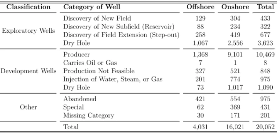
Agˆencia Nacional do Petr´oleo, G´as Natural e Biocombust´ıveis (ANP), the Brazilian oil and gas industry regulator. The dataset contains detailed information on the universe of wells drilled in Brazil: 20,052 wells spanning the years from 1940 to 2000. The dataset contains the location (latitude and longitude) of each well, the exact date of the drilling, and the result (whether oil was found, whether the well is a dry hole, whether only water was found, among others). Furthermore, we have information on the viability of exploring the oil deposit (when oil was found), and on whether the oil company started production by drilling production wells.
Table 1 shows the number of wells by category. Drilled wells are classified according to the result of the attempt to find oil. A drilled well can be classified, among other categories, as a discovery well, a producer well, a dry hole, or an abandoned well (e.g., because of an accident).10 However, wells can be broadly classified as exploratory wells
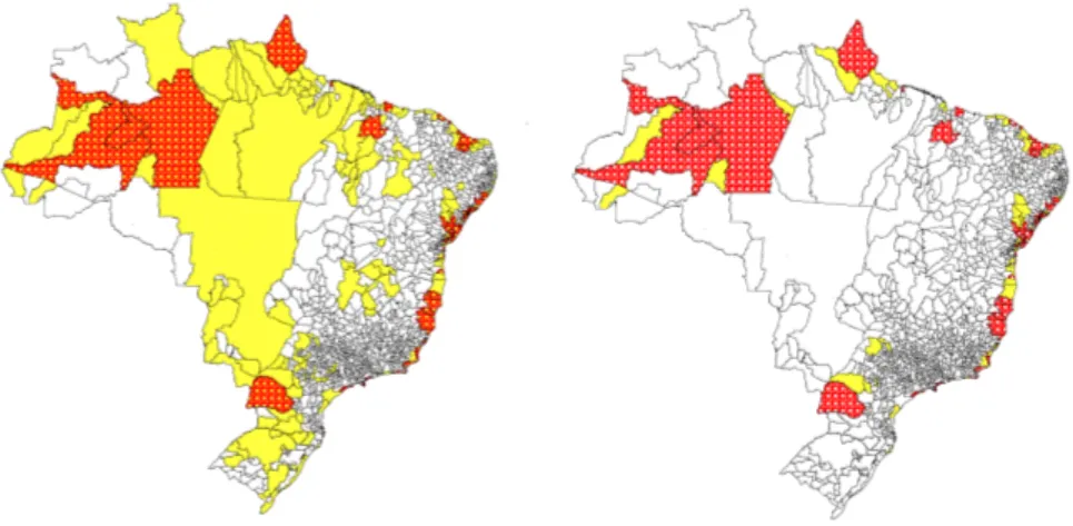
and development wells. Exploratory wells are drilled to test for the presence of oil, while wells drilled inside the known extent of the field are called development wells (e.g., pro-ducer wells). Unsuccessful drilling is classified as a dry hole in both exploratory and development categories.11 Figure1shows the geographic distribution of drilling and
dis-coveries in Brazil and highlights that oil drilling in Brazil is concentrated in sedimentary basins (which is where oil can potentially be found – see Section 4).
To match wells and MCAs we proceed as follows. For onshore wells, we simply allocate the wells to the MCAs within whose boundaries they were located. For offshore wells, we calculate the distance from each well to the nearest coastal MCA and allocate the offshore well to that MCA.12
Local Economic Development: 1940–2000. We combine data from several
sources to obtain as much information as possible on measures of local economic de-velopment in Brazil. In order to construct historical outcomes at the municipal level, we use two main data sources: Population Censuses and Economic Censuses.
The Population Censuses provide us with a reliable long-running source of information on population characteristics at the municipal level. From the Population Censuses (of 1940, 1950, 1960, 1970, 1980, 1991, 1996, and 2000), we obtained data on population
1940. The number of municipalities was the same in 1997 and 2000. Additional information on MCA aggregation can be found inReiset al. (2007) andDa Mataet al. (2007).
10
We obtained more the 50 different classifications from the dataset, but we were able to aggregate all of them into a few major categories (see Table1). The data differentiate between oil well, gas well, and oil and gas well. One limitation of the dataset is that it does not include information on the amount of oil produced by each individual producer well during the period of interest. Data on well production are available only from the the 2000 onward.
11
See AppendixB.1for a detailed explanation of the types of wells.
12
Table 1: Number of Wells by Category
Classification Category of Well Offshore Onshore Total
Exploratory Wells
Discovery of New Field 129 304 433
Discovery of New Subfield (Reservoir) 88 234 322 Discovery of Field Extension (Step-out) 258 419 677
Dry Hole 1,067 2,556 3,623
Development Wells
Producer 1,368 9,101 10,469
Carries Oil or Gas 7 1 8
Production Not Feasible 327 521 848 Injection of Water, Steam, or Gas 201 774 975
Dry Hole 73 1,017 1,090
Other
Abandoned 421 554 975
Special 62 369 431
Missing Category 30 171 201
Total 4,031 16,021 20,052
Notes. Data from ANP (Brazilian oil and gas industry regulator). Wells are classified broadly as exploratory wells and development wells. Exploratory wells are drilled to test for the presence of oil. If the exploratory drilling was proven unsuccessful, the well is classified as a dry hole. Wells to delineate the extension of the oil field (step-out wells) are also classified as exploratory wells. Every well drilled inside the known extent of the field is called a development well (e.g., producer wells and injection wells). In the development well category, unsuccessful drilling is also classified as a dry hole. Special wells are water wells or the ones used for mineral research and experiments.
counts, population density, urbanization rate, and employment.13 We group sectoral
employment categories so that they are consistent over time. We obtain the following six categories: (i) agriculture and fishing, (ii) manufacturing including extractive activities, (iii) retail, (iv) transportation, (v) public sector and (vi) services.
Gross Domestic Product (GDP) data are from Economic Censuses (of 1949, 1959, 1970, 1975, 1980, and 1985), sector surveys in 1996, and from the national accounts of 2000. Reis et al. (2004) constructed municipal-level GDP from historical Economic Censuses, from where it is possible to calculate GDP through the production approach. Since 1949, the Censuses provide data on the value of total outputs and total costs (a proxy for intermediate goods) at the municipal level. More precisely, the Censuses provide total output and total input by economic sector so it is possible to construct value-added figures by sector. Sectoral GDPs were then added so as to calculate the total municipal GDP. Oil and Mining were included in the manufacturing GDP. The municipal GDP is deflated using the national implicit price deflator.14
Microdata. To improve on the analysis, we use cross-sectional microdata for the
year 2000. We use a matched worker–firm dataset from the Ministry of Labor’s RAIS (Rela¸c˜ao Anual de Informa¸c˜oes Sociais). The RAIS data have been collected annually since the late 1980s but are considered to be of high quality only since the mid 1990s. Since the population census data are collected once per decade, 2000 is the first year in which reliable RAIS data overlapped with a population census. The RAIS dataset has information on each formal worker at each plant in Brazil. In 2000, there were 36,907,953
13
Densities are specified as population per square kilometer. The urbanization rate is the proportion of the population living in urban areas.
14
Fig. 1: Oil Wells in Brazil: 1940-2000
(a) Oil Wells: Discovery (red) vs. dry (yellow) (b) Sedimentary Basins (light green)
Notes. The figures show the locations of approximately 20,000 drilled wells (the universe of wells drilled in Brazil during the period from 1940 to 2000). In Figure1(a), wells with Oil Discovery are in red, Dry Wells are in yellow, and others are in white. Figure1(b)shows the locations of sedimentary basins in Brazil (in light green). Both figures show the
administrative boundaries of the 27 states of Brazil that have been in effect since 1988. (See
https://www.youtube.com/watch?v=_ZKdnUeBcOIfor a short video on the geographic distribution of drilling activity in Brazil from 1940 to 2000.)
formal workers in the dataset. We use this information to construct measures of average wages, as well as the numbers of workers and firms by skill and sector at the municipal level. We also calculate firm density and worker density, which are specified as the number of firms and workers, respectively, per square kilometer. Since RAIS only covers workers in the formal sector, we complement it with microdata from the 2000 Population Census, which allow us to obtain the fraction of workers employed in the formal sector.
Geography. Data on average temperature, average rainfall, and average altitude
come from Ipeadata.15 Further data comprise the latitude and longitude of each MCA,
distance to the closest state capital, as well as geographical indicators of its location (on the coast, in the Amazon region, and in the semiarid region).16
2.1
Stylized Fact: A First Look at the Data
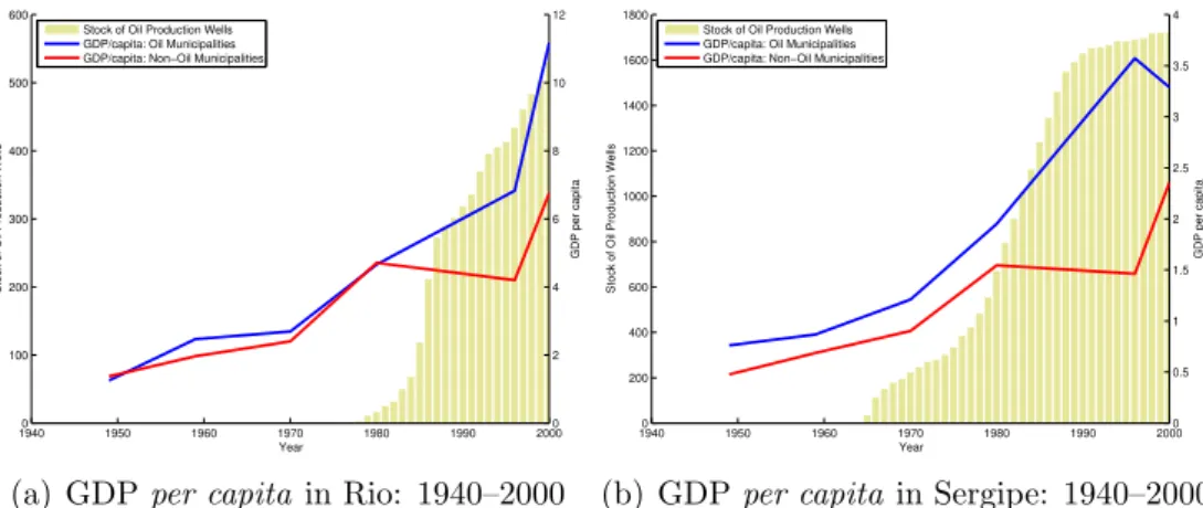
Figures 2(a) and 2(b) show GDP per capita for the period 1940–2000 in the states of Rio de Janeiro and Sergipe (two important oil-producing states in Brazil), respectively. For each state, the graphs illustrate the evolution of GDP of municipalities with and
15
Temperature is measured in degrees Celsius, precipitation in millimeters per month, and altitude in meters.
16
without oil. It can be seen that a wedge in GDP per capita between oil-producing municipalities and those without oil production emerged over the years. Furthermore, the timing appears to correspond quite closely to the development of the oil sector in each state. At first glance, oil production appears to have substantially increased local GDP. Two questions naturally arise from this. Firstly, is the observed correlation causal? And secondly, how did the non-oil sector develop? Since oil extraction is a high-value-added activity, local GDP increases mechanically when oil is produced, bar any extreme “Dutch Disease” effect. We are interested in assessing which non-oil sectors are affected and whether the spillovers of oil production to other sectors are positive or negative.
Fig. 2: GDP per capita in Oil and Non-Oil Municipalities
19400 1950 1960 1970 1980 1990 2000
100 200 300 400 500 600 Year
Stock of Oil Production Wells
0 2 4 6 8 10 12
GDP per capita
Stock of Oil Production Wells GDP/capita: Oil Municipalities GDP/capita: Non−Oil Municipalities
(a) GDPper capita in Rio: 1940–2000
19400 1950 1960 1970 1980 1990 2000
200 400 600 800 1000 1200 1400 1600 1800 Year
Stock of Oil Production Wells
0 0.5 1 1.5 2 2.5 3 3.5 4
GDP per capita
Stock of Oil Production Wells GDP/capita: Oil Municipalities GDP/capita: Non−Oil Municipalities
(b) GDPper capita in Sergipe: 1940–2000
Notes. Figure showsper capitaGDP in municipalities of the states of (a) Rio de Janeiro and (b) Sergipe in which oil was discovered during the period 1940 to 2000 (blue line) and those in which it was not (red line). Rio de Janeiro is the most important producer (in terms of volume of oil), and the first oil discovery there took place in the late 1970s. The first commercial oil well in Sergipe was discovered in the mid 1960s.
3
The Empirical Model
We aim to recover the impact of oil on economic development at the local level. We present the basic regression model in this section, and discuss the quasi-experiment we exploit to obtain a causal coefficient in Section 4. Let Yit be a measure of economic
development in MCA i and year t. Our empirical model is the following Difference-in-Difference specification
Yit =α+τ Tit+βt′Xi+γi+ρt+ǫit, (1)
whereXi are time-invariant MCA characteristics, including the pre-treatment level of the
dependent variable,ǫit is an error term,ρt denotes year fixed effects andγi denotes MCA
for shocks common to all Brazilian MCAs, while the MCA fixed effects capture time-invariant MCA characteristics such as location, geology, or distance to the coast. Some of those time-invariant geographic characteristics might have time-varying effects (the importance of being located on the Coast might have increased as Brazil was integrated more closely into the world economy, for example). To address this we explicitly include longitude, latitude, an indicator for being located in the Amazon, and an indicator for being located on the coast in the vector of controls Xi and allow for time-varying
coef-ficients βt. We also include measures of economic development in 1940 (before the first
successful oil discovery) in Xi to capture initial conditions. In general, we use the
loga-rithm of a measure of economic development as the dependent variable so thatτ gives us the percentage points difference in outcomes over a period of up to 60 years between a municipality which produces oil and one that does not. Lastly, note that policy variation takes place at the MCA level, and errors within the spatial units may be correlated. Therefore, standard errors are clustered at the MCA level in all regressions (Bertrand
et al. (2004)).
4
The Oil Lottery: A Quasi-Experiment
An estimation of Equation (1) above would expose our results to a major concern as oil production is likely to be endogenous to local economic conditions. For example, production might be more attractive close to large urban centres, might be influenced by strategic behavior regarding production quota, or might occur in some regions but not others because of political economy considerations. The endogeneity related to production might even be more problematic because the transportation of oil (and gas) requires a substantial investment in infrastructure such as pipelines.
A first step to address the endogeneity issue is to use discoveries instead of production as the explanatory variable. Discoveries are arguably more exogenous than production. This might not go a long way in overcoming endogeneity concerns, however. Recent papers such as Cust and Harding (2014) show that institutions are an important driver of oil exploration and therefore of discoveries. We therefore need to take a further step back to try and identify exogenous variation in discoveries. We obtain this exogenous variation by exploiting the quasi-experiment generated by the randomness in the success of exploratory oil drilling. In other words, our key identifying assumption is that con-ditional on exploratory drilling taking place, a discovery is unrelated to local economic conditions. In practice, in the regression analysis we thus restrict our sample of munici-palities to those with drilling. Municimunici-palities with drilling and no discoveries constitute the control group, and those with discoveries are assigned to treatment.
identifying assumption qualitatively. Third, we conduct formal tests of a lack of correla-tion between discoveries condicorrela-tional on drilling and local economic condicorrela-tions to justify the identifying assumption quantitatively. Fourth and last, we discuss implementation.
4.1
The Institutional Setting in Brazil
The Brazilian oil sector has experienced substantial development from 1940 onwards. In 1939, the first onshore field (which was non-commercial) was discovered, and in 1941 the first viable onshore well was drilled. The first oil discovery from an offshore well took place in 1968. Figure3summarizes domestic and international events related to oil exploration and production in Brazil.17
Fig. 3: Events and Oil Drilling: 1940–2011
19400 1950 1960 1970 1980 1990 2000 2010 20 40 60 80 100 Year
Cumulative Wells (\%)
1941: First Discovery 1953: Petrobras 1968: First Offshore Discovery 1973: First Oil Shock 1979: Second Oil Shock 1997: Market open to
private oil companies
2006: Self− Sufficiency
Notes. Figure shows the cumulative percentage of oil wells drilled in Brazil during the period from 1940 to 2011.
During most of our period of interest, only government-owned entities were able to explore and produce oil in Brazil. In 1938, under a dictatorship that lasted from 1937 to 1945, Federal Law n. 395/38 established state control of oil development, and not until 1997 (Federal Law n. 9,478/97) were private companies allowed to autonomously explore and produce oil in Brazil. Federal Law n. 395/38 created the CNP (in Portuguese,
Conselho Nacional do Petr´oleo), the only entity responsible for exploring oil from 1938 to 1953.18 From 1953 to 1997, only one company was allowed to drill for oil in Brazil: the
government-controlled Petrobras.19 Petrobras is an integrated exploration and production
17
In 2011, Brazil was the world’s 13th largest producer of oil and gas, with 2.2 millon barrels per day, which represents 2.6% of the total produced worldwide. Brazil has the world’s 14th largest proven petroleum reserves in the same year (ANP(2012)).
18
According to Federal Law n. 395/38, private oil companies could operate only via concessions granted by the CNP. Anecdotal evidence suggests that it was difficult for a private oil company to operate in Brazil at that time.
19
company whose activities encompass all phases of the oil supply chain.
Royalties did not play an important role for local government finances for most of our sample period. Only in 1997 a change in the allocation rule led to huge increases in royalty payments to municipalities and turned them into a key source of local government revenue. Prior to the reform, royalties accounted for roughly 3 percent of municipal budgets in oil producing municipalities. This allows us to claim that in our analysis we will identify mainly the direct impact of oil production on local economic development rather than the indirect impact via a fiscal windfall (seeB.2 for more details on royalties in Brazil).
4.2
The Success of Oil Drilling as a Randomization
Oil and gas exploration is known to be a risky business. Oil companies aim to find an oil field, which corresponds to a contiguous geographic area with oil, and they thus search for areas with specific geological characteristics to drill for oil. For instance, oil companies search for areas that contain geological structures (subsurface contortions and specific rocks) for potential trapping of hydrocarbons. Geology and related disciplines provide guidance on where to search for oil traps, and estimating the probability of discovery prior to drilling is an important aspect of petroleum exploration. However, only by drilling can the company be certain that hydrocarbon deposits really exist. Even with modern technology, the only direct way of confirming the hypothesis of oil presence is by drilling a well. Oil companies may invest substantially in acquiring information, only to end-up with either no discoveries or none that are profitable.
The likelihood of finding oil from drilling can be low, even in areas with appropriate geological characteristics, and learning-by-doing is an important aspect of the petroleum industry (Kellogg (2011)). Testing by drilling is expensive and may not reduce the un-certainty regarding the existence of oil. Numbers vary, but in a newly explored area the likelihood of successfully drilling for oil can be very low, and subjective probabilities are widely accepted in the petroleum industry (Harbaughet al.(1995)).20 Even with modern
technology, drilling is not a “safe bet,” since there is no guarantee that a company will find oil after drilling. Given the features of drilling, oil discovery depends both on geolog-ical characteristics and on “luck.”21 Our data support the idea that discovering oil can
be viewed as a “lottery” (where drilling for oil is akin to buying the lottery ticket): For every exploration well drilled which was successful, there were many more unsuccessful ones – a ratio of roughly one over four (recall Table1 in Section 2).
Petrobras is one of the largest oil companies in the world and a leading company in oil exploration, with contributions to technology, especially for deep-water exploration.
20
Today, an exploration well (wildcat well – a well drilled a mile or more from an area of existing oil production) can have a probability as low as 10% of yielding viable oil, while a rank wildcat (a well drilled in an area where there is no existing production) has an even smaller chance of finding oil.
21
4.3
The Identifying Assumption in Practice
Is drilling success unrelated to local economic activity? Using the well data, we
first generate an indicator variable to separate places where drilling took place (J = 1) from places with no drilling (J = 0). We then restrict our analysis to municipalities for which J = 1. For all those municipalities with drilling we then construct an indicator for whether a discovery was made (Z) and another for whether oil is produced (T). As a first step, we created two different dummy variables for discovery (Z) and a dummy for well production (T). The dummy for production follows immediately from the well data – it is set equal to one when there is at least one producer well in the municipality. In terms of discoveries, there are several possibilities, as the data allow us to differentiate between a field discovery, a subfield (reservoir) discovery, and a field extension discovery. We define two different discovery dummies as follows. The first dummy (“All Discoveries”) is set equal to one when at least one field, subfield, or field extension discovery was made in the municipality. The second dummy (“True Discoveries”) is set equal to one when at least one field or subfield discovery and at least one field extension discovery were made in the municipality. The rationale for the latter is that any meaningful discovery includes a field or subfield discovery and subsequent field extension discoveries to delineate the size of the oil field (see Appendix B.1).
We thus obtain the following numbers regarding assignment to treatment:
• Total number of MCA units = 1,275
• Drilling MCAs = 222
• All Discoveries MCAs = 64
• True Discoveries MCAs = 45
Table 2 provides some evidence that the success of oil drilling is exogenous to local economic conditions. We regress (i) the number of exploratory wells with a discovery between 1940–2000 and (ii) the ratio of successful drilling to unsuccessful drilling in the same period on pre-treatment characteristics. We find that both the number of discoveries and drilling success ratio are unrelated to pre-treatment local economic characteristics. It is in fact particularly reassuring that the success ratio is uncorrelated with all controls (Column (3)). That is, conditional on drilling taking place, success seems to be truly a lottery.
an alternative control group where we include only those municipalities with the best co-variate overlap with the assigned to treatment group. This is discussed in detail below in this subsection.
Table 2: Discoveries, Conditional on Drilling
(1) (2) (3)
Dependent variable: Number of Discovery Wells Drilling Success Ratio
OLS
Poisson Linear
Probability
Urbanization in 1940 0.741 -0.814 0.120
(9.777) (1.562) (0.125)
Log of Pop. Density in 1940 2.771 0.416 -0.0145
(2.499) (0.347) (0.0247)
GDPper capitain 1949 2.959 0.548 -0.00265
(2.239) (0.344) (0.0288)
Ln Worker Density in 1940 -2.436 -0.298 0.0129
(2.857) (0.384) (0.0247)
Semiarid Indicator 10.80 1.389** 0.102
(7.663) (0.545) (0.0689)
Amazon Indicator 2.761 -0.335 -0.0274
(4.005) (0.814) (0.0642)
Coastal Indicator 10.84** 1.732*** 0.0596
(5.456) (0.667) (0.0425)
Distance to closest state capital (km) 0.000687 0.000501 4.49e-06
(0.0105) (0.00225) (0.000152)
Constant -1.853 0.358 0.0731
(4.300) (0.837) (0.0464)
Observations 222 222 210
R-squared 0.071 - 0.031
Notes. Robust standard errors in parentheses. The regressions are for the 222 Minimum Comparable Areas (MCAs) in which Petrobras drilled for oil. The dependent variables are the number of discovery wells in 1940–2000 and the drilling success ratio in 1940–2000. The drilling success ratio is the ratio of exploratory wells with oil to exploratory dry wells.
*** p<0.01, ** p<0.05, * p<0.1
It is also useful to check whether conditional on a first discovery, additional drilling attempts (and thus discoveries) are unrelated to local economic development. Specifi-cally, if Petrobras, following an initial discovery, tried harder to find a field extension discovery in a location which was growing fast, or which had high demand, this could bias our results (in particular, when using the “True Discovery” dummy). Table3shows that this is not the case. Unsurprisingly, drilling attempts increase significantly after an initial discovery was made in an MCA. A first discovery is a strong signal, and natu-rally Petrobras subsequently intensifies its efforts in that particular area. Importantly, however, there is no indication that drilling increases more in MCAs with higher GDP
per capita, more urbanized MCAs, more densely populated ones, or MCAs with a higher employment density.
The Overlap between the assigned to treatment and control groups. As
Table 3: Drilling, Conditional on a Field Discovery
(1) (2) Dependent variable: Wells drilled per year
Estimation: OLS Poisson
Field Discovery Dummy 5.502** 5.255*** (2.259) (0.514) Field Discovery Dummy * log Population Density -0.517 -0.0689 (0.600) (0.0721) Field Discovery Dummy * log GDP/capita 0.849 0.107
(1.121) (0.135) Field Discovery Dummy * Urbanization 4.706 0.690
(5.925) (0.829) Field Discovery Dummy * log Worker Density 4.706 0.690
(5.925) (0.829)
Constant 0.0285*** -3.557***
(0.0104) (0.366)
Observations 5,098 5,098
Notes. Robust standard errors in parentheses. The regressions are for 1,275 Minimum Comparable Areas (MCAs). The dependent variable is the count of drills per year. The explanatory variables are a dummy for a field discovery and the interactions between this dummy and GDP/capita, urbanization, and population density. *** p<0.01, ** p<0.05, * p<0.1
two groups. Imbens and Wooldridge (2009) point out that for limited covariate overlap between the treatment and control group “linear regression methods tend to be sensitive to the specification” (p. 24). We thus use the normalized (or standardized) difference to assess the differences in the covariate distributions between the two groups (Rubin(2001) and Imbens and Wooldridge (2009)).22
As can be seen in Table 4, and as Table 2 already indicated, the overlap between the assigned to treatment and control group is not ideal for certain geographic variables. While the overlap is good for initial economic conditions, discoveries turn out to be disproportionately located on the coast and in the Amazon region relative to locations with dry drilling. To improve overlap, we created a matched subsample of the “drilling but no discovery” group. Propensity score matching (or trimming) is a common way to improve overlap (Imbens and Wooldridge(2009)). For this subsample, we choose the 64 municipalities with the highest propensity score and call this control group “matched dry drilling.”23 Figure 4shows maps with the locations of the two control groups we obtain.
Figure 4(a) shows the places with discoveries and the set of MCAs where drilling took place and no oil was found. Figure 4(b) displays the matched dry-hole subpopulation. We will later show that in practice it makes little difference to the results which control group we use.
22
Standardized differences are not influenced by sample size, unlike t-tests and other statistical tests. Imbens and Wooldridge(2009) suggest that the normalized difference should be below 0.25.
23
Table 4: Overlap between Assigned to Treatment and Control Groups
(I) (II) (III)
Variable Oil Discovery Dry Matched Dry
Drilling Drilling
Pop. Density 1940
Mean 32.89 30.33 35.09
S.D. 51.35 132.29 104.47
Standardized Difference - 0.018 -0.019
Urbanization 1940
Mean 0.27 0.22 0.24
S.D. 0.18 0.18 0.2
Standardized Difference - 0.196 0.111
GDP per capita 1949
Mean 0.67 0.88 0.69
S.D. 0.42 0.89 0.75
Standardized Difference - -0.213 -0.023
Manufacturing/GDP 1949
Mean 0.19 0.13 0.13
S.D. 0.15 0.16 0.17
Standardized Difference - 0.274 0.292
Services/GDP 1949
Mean 0.38 0.37 0.4
S.D. 0.2 0.21 0.23
Standardized Difference - 0.034 -0.066
Agriculture/GDP 1949
Mean 0.43 0.51 0.48
S.D. 0.24 0.24 0.26
Standardized Difference - -0.236 -0.141
Worker Density 1940
Mean 10.83 9.75 10.8
S.D. 16.78 43.35 29.65
Standardized Difference - 0.023 0.001
Share of Workers in Services Sector 1940
Mean 0.078 0.064 0.073
S.D. 0.055 0.058 0.065
Standardized Difference - 0.166 0.046
Share of Workers in Public Sector 1940
Mean 0.015 0.016 0.019
S.D. 0.014 0.019 0.024
Standardized Difference - -0.034 -0.125
Avg. Rainfall
Mean 118.46 127 122.23
S.D. 38.79 43.65 51.44
Standardized Difference - -0.146 -0.059
Avg. Temperature
Mean 24.95 23.96 24.35
S.D. 1.9 2.97 2.7
Standardized Difference - 0.281 0.182
Latitude
Mean -11.88 -13.72 -12.62
S.D. 6.44 9.67 8.6
Standardized Difference - 0.158 0.069
Longitude
Mean -40.65 -46.94 -43.5
S.D. 6.46 7.31 7.6
Standardized Difference - 0.645 0.286
Coastal Indicator Prop. 0.59 0.3 0.53
Standardized Difference - 0.431 0.086
Semiarid Indicator Prop. 0.19 0.15 0.23
Standardized Difference - 0.075 -0.070
Amazon Indicator Prop. 0.08 0.3 0.17
Standardized Difference - -0.413 -0.194
Number of MCAs 64 158 64
Fig. 4: Treatment and Control Groups
(a) Discovery (Red), Drilling (Yellow) (b) Discovery (Red) and Matched Dry Drilling Sample (Yellow)
Notes. Figures show 1,275 Minimum Comparable Areas (MCAs) in 1940. The discovery dummy is the “All Discoveries” dummy (which is equal to one when at least one field, subfield, or field extension discovery was made in the MCA).
4.4
Implementation
We now briefly discuss the empirical model we use to recover the impact of oil discoveries. The estimand of interest is the Intention-to-Treat (ITT): the average impact of being assigned to treatment. Let yi be the potential outcome for local economy i, and let the
indicator of treatment assignment be Zi = {0,1}. The ITT estimand is represented by
ITT =E[yi|Zi = 1]−E[yi|Zi = 0].
In the discussion below, the oil discovery dummy is represented byZit (our treatment
assignment), which is set equal to 1 if oil was discovered in MCA unit i in period t ≥
¯
t, where ¯t is the time of the discovery. We assume an additive and linear empirical specification to estimate an ITT effect, as follows:
Yit =α+τI T TZit+β
′
tXi+γi+ρt+ǫit, (2)
Later on in the analysis we will use discoveries to instrument for production to recover a coefficient which can be interpreted as a Local Average Treatment Effect (LATE).
5
Results
5.1
Baseline Results
Socio-Economic Variables. Table5shows the baseline ITT results using the “All
worker density, which are expressed as logs. Therefore, the coefficient in those regres-sions can be interpreted as a percentage change. An additional dependent variables is the urbanization rate, which is bounded between 0 and 1, so that the coefficient for oil discov-eries can be interpreted as a change in percentage points. GDP per capita increased by 12.5–14.6% over a 60-year period as a result of oil discoveries. Population density, worker density, and the urbanization rate are unaffected by oil discoveries in this specification.
Table 5: Intention-to-Treat Effect of All Oil Discoveries: Socio-Economic Outcomes
Dry Drilling Matched Dry Drilling
(1) (2) (3) (4) (5) (6) (7) (8)
VARIABLES ln ln ln Urbaniz- ln ln ln
Urbaniz-GDP Population Workers ation GDP Population Workers ation
per capita Density Density Rate per capita Density Density Rate
Discovery Dummy 0.125* -0.0390 -0.0720 0.0283 0.146* -0.0400 -0.0720 0.0253
(0.0728) (0.0579) (0.0669) (0.0187) (0.0783) (0.0626) (0.0669) (0.0199)
MCA FE Yes Yes Yes Yes Yes Yes Yes Yes
Year FE Yes Yes Yes Yes Yes Yes Yes Yes
Observations 1,332 1,776 1,330 1,776 768 1,024 1,330 1,024
Number of MCAs 222 222 222 222 128 128 222 128
Geographical Controls Yes Yes Yes Yes Yes Yes Yes Yes
Initial Conditions Yes Yes Yes Yes Yes Yes Yes Yes
Estimation FE FE FE FE FE FE FE FE
Notes. Standard errors clustered at the MCA level. Geographical controls and initial conditions have time-varying coefficients. *** p<0.01, ** p<0.05, * p<0.1
As discussed earlier, the “All Discovery” dummy has some drawbacks, both conceptu-ally and in terms of its ability to predict oil production. The “True Discoveries” dummy excludes both MCAs where oil was discovered but there were no follow-up discoveries (i.e., the oil field was very small) and MCAs where there was no field discovery but only a field extension (i.e., the bulk of the field lies in a different municipality).24
Table 6 shows the baseline ITT results using our preferred treatment assignment (“True Discoveries”). Unsurprisingly, the coefficients are markedly higher than in Table5. The increase inper capitaGDP is estimated at 24.6–25.9%. While population density and worker density are not significantly affected, urbanization increases by 4.3–4.4% points over the period as a consequence of oil discoveries. In other words, when we compare municipalities with meaningful discoveries to municipalities where Petrobras drilled for oil and either did not find any or made no substantial discovery, we find a strong positive impact on per capita GDP and urbanization.
Sectoral GDP and Sectoral Employment Shares. To understand whether the
increase in GDP per capita is purely mechanical, in the sense that there are no spillovers from oil production to other sectors of the economy, we investigate the impact of oil
24
Table 6: Intention-to-Treat Effect of True Oil Discoveries: Socio-Economic Outcomes
Dry Drilling Matched Dry Drilling
(1) (2) (3) (4) (5) (6) (7) (8)
VARIABLES ln ln ln Urbaniz- ln ln ln
Urbaniz-GDP Population Workers ation GDP Population Workers ation
per capita Density Density Rate per capita Density Density Rate
Discovery Dummy 0.246*** -0.00864 -0.0475 0.0443** 0.259*** -0.0127 -0.0394 0.0430**
(0.0856) (0.0676) (0.0758) (0.0202) (0.0910) (0.0731) (0.0814) (0.0213)
MCA FE Yes Yes Yes Yes Yes Yes Yes Yes
Year FE Yes Yes Yes Yes Yes Yes Yes Yes
Observations 1,332 1,776 1,330 1,776 768 1,024 767 1,024
Number of MCAs 222 222 222 222 128 128 128 128
Geographical Controls Yes Yes Yes Yes Yes Yes Yes Yes
Initial Conditions Yes Yes Yes Yes Yes Yes Yes Yes
Estimation FE FE FE FE FE FE FE FE
Notes. Standard errors clustered at the MCA level. Geographical controls and initial conditions have time-varying coefficients. *** p<0.01, ** p<0.05, * p<0.1
discoveries on sectoral GDP in Table7.25 GDP is broken up into manufacturing, services,
and agriculture. Natural resource extraction is included in the manufacturing sector. While ideally we would like to decompose this further, the available data does not allow us to do so. As such, it is not surprising that manufacturing GDP increases significantly with oil discoveries. Importantly, however, services GDP increases by about 20%, while agricultural GDP is unaffected (the point estimate is negative but insignificant).
Table 7 (Columns (4)–(9)) also looks at how sectoral employment shares are affected by discoveries and finds results consistent with the estimated impact on sectoral GDP. We find that in oil municipalities an important structural transformation occurs: workers reallocate from the agricultural sector to the services sector. To a lesser degree, the share of workers in the public sector also increases. A plausible hypothesis is that local demand for non-tradables from well paid oil workers and the oil company lead to an expansion of the services sector which attracts rural agricultural workers to move to the local urban agglomeration. At the same time additional local government revenues allow the municipal government to expand employment.
Onshore versus Offshore Discoveries. Distinguishing between onshore and
off-shore discoveries allows us to study this possibility in more detail. In particular, some of the channels which we believe can lead to spillovers (such as the physical presence of well-paid oil workers) might be more obviously present for onshore than for offshore loca-tions. In fact, offshore production is concentrated largely off the coast of Rio de Janeiro, and most personnel associated with offshore production is stationed in only one location (the municipality of Maca´e).
25
Table 7: Intention-to-Treat Effect of Oil Discoveries: Sectoral GDP and Sectoral Employment
Matched Dry Drilling
(1) (2) (3) (4) (5) (6) (7) (8) (9)
Sectoral GDP Sectoral Employment: Shares
VARIABLES ln Agriculture ln Manufacturing ln Services Agricult- Manufact- Retail Transport- Public Services
GDPper cap GDPper cap GDPper cap ure uring ation Sector
Discovery Dummy 0.0664 0.456** 0.215** -0.0419* -0.00768 0.00152 0.00266 0.00947*** 0.0359***
(0.109) (0.189) (0.104) (0.0223) (0.0151) (0.00457) (0.00313) (0.00305) (0.0114)
MCA FE Yes Yes Yes Yes Yes Yes Yes Yes Yes
Year FE Yes Yes Yes Yes Yes Yes Yes Yes Yes
Observations 765 764 765 767 767 767 767 767 767
Number of MCAs 128 128 128 128 128 128 128 128 128
Geographical Controls Yes Yes Yes Yes Yes Yes Yes Yes Yes
Initial Conditions Yes Yes Yes Yes Yes Yes Yes Yes Yes
Estimation FE FE FE FE FE FE FE FE FE
Notes. Standard errors clustered at the MCA level. Geographical controls and initial conditions have time-varying coefficients. Discovery is defined as “True Discovery”. *** p<0.01, ** p<0.05, * p<0.1
The disaggregated results for onshore and offshore discoveries are shown in Table8(in Columns (1)–(10)). For onshore discoveries we use municipalities with onshore drilling and no discoveries as the control group, while for offshore discoveries we use municipalities with offshore drilling and no discoveries as the control group. Municipalities with both onshore and offshore drilling are excluded from the analysis.
We find a large positive impact of onshore discoveries on local economic development but no impact of offshore discoveries. In fact, for offshore discoveries the coefficients are estimated to be equal to zero with some precision in Columns (6)–(10). For manufacturing GDP per capita the estimated coefficient is positive but not significantly. For onshore discoveries, services GDP per capita increases by 36%, the urbanization rate increases by over 8 percentage points, while the fraction of services workers in the local economy increases by over 5 percentage points. Additionally, the fraction of public sector workers increases by roughly 1 percentage point. We interpret these results as support for the hypothesis that a structural shift towards the services sectors is caused by a local demand shock in municipalities with onshore discoveries. Since this demand shock is absent after offshore discoveries there is no effect there. The impact on public sector employment might be due to two factors: first, there was a (very) small impact on government revenues even before 1997 due to royalties. In 1995, the first year for which we have data on royalties at the municipal level, they made up 2.84 percent of government revenue for onshore municipalities. Second, the increase in local activity generated additional local revenues via local tax collection. Property taxes, for example, are collected locally and could have benefited from the increased urbanization.26
Historical vs. Contemporaneous Effects. To gain additional insights, we split
discoveries into pre- and post-1970. 1970 is a somewhat arbitrary cut-off based on the mid-point of our sample period. As virtually all offshore discoveries took place after 1970, this exercise essentially allows us to split the onshore discovery sample to explore the medium-run versus long-run effects of oil discoveries. It has the additional advantage that it allows us to verify whether the difference in results between onshore and offshore discoveries is simply due to different timing of the discoveries.
Columns (11)–(15) of Table 8 show how onshore discoveries before and after 1970 impact our relevant outcomes. Pre-1970 discoveries are associated with significantly larger coefficients. They have led to large increases in GDP per capita, urbanization,
26
Table 8: Onshore versus Offshore Discoveries
Control Group: Dry Drilling Onshore Control Group: Dry Drilling Offshore Control Group: Dry Drilling Onshore
(1) (2) (3) (4) (5) (6) (7) (8) (9) (10) (11) (12) (13) (14) (15)
VARIABLES ln GDPper capita Urbanization Employment Share ln GDPper capita Urbanization Employment Share ln GDPper capita Urbanization Employment Share
Manufact- Services Rate Services Public Manufact- Services Rate Services Public Manufact- Services Rate Services Public
uring Sector uring Sector uring Sector
Onshore Discovery 0.632** 0.359** 0.0866** 0.0585** 0.00909**
(0.272) (0.117) (0.0245) (0.0131) (0.00389)
Offshore Discovery 0.206 0.0488 -0.00098 0.027 0.00571
(0.332) (0.233) (0.0487) (0.0234) (0.00435)
Onshore Discovery * Pre-1970 0.684* 0.545*** 0.0967*** 0.0788*** 0.0080*
(0.395) (0.156) (0.0356) (0.0171) (0.0048)
Onshore Discovery * Post-1970 0.554 0.0842 0.0698*** 0.0239** 0.011*
(0.357) (0.112) (0.0220) (0.0114) (0.0061)
MCA FE Yes Yes Yes Yes Yes Yes Yes Yes Yes Yes Yes Yes Yes Yes Yes
Year FE Yes Yes Yes Yes Yes Yes Yes Yes Yes Yes Yes Yes Yes Yes Yes
Observations 1,007 1,003 1,352 1,012 1,012 322 324 432 320 320 1,007 1,003 1,352 1,012 1,012
Number of MCAs 169 169 169 169 169 54 54 54 54 54 169 169 169 169 169
Geographical Controls Yes Yes Yes Yes Yes Yes Yes Yes Yes Yes Yes Yes Yes Yes Yes
Initial Conditions Yes Yes Yes Yes Yes Yes Yes Yes Yes Yes Yes Yes Yes Yes Yes
Estimation FE FE FE FE FE FE FE FE FE FE FE FE FE FE FE
Notes. Standard errors clustered at the MCA level. Geographical controls and initial conditions have time-varying coefficients. The control group in Columns (1)–(5) and in Columns (11)–(15) is the group of municipalities with onshore drilling and no discoveries (“Dry Drilling Onshore”). The control group in Columns (6)–(10) is the group of municipalities with offshore drilling and no discoveries as the control group (“Dry Drilling Offshore”).
*** p<0.01, ** p<0.05, * p<0.1
workers in the services sector, and workers in the public sector. Post 1970 onshore discoveries have a similarly sized point estimate on manufacturing GDP (as one would expect if production volumes are similar across the two groups) but the coefficient is imprecisely estimated. The results suggest that later discoveries increase urbanization and the share of workers in the services sectors by only about 60 percent and 30 percent as much as earlier discoveries. While power is a concern in these regressions, the results nevertheless offer some indicative evidence for long-run agglomeration effects associated with oil discoveries. Additionally, we can rule out that the lack of impact associated with offshore discoveries is purely a matter of the timing of the discoveries.
To study the impact of discoveries on non-oil manufacturing and to understand the impact on the services and agricultural sectors at the worker and firm level in more detail, we turn to matched employer-employee data in Subsection 5.4. We employ a cross-sectional specification, given that the data are not available in the long time series which we used so far. Prior to exploring the underlying mechanisms in more detail in that way, however, we check the robustness of our baseline results (Subsection 5.2) and then obtain coefficients which can be interpreted as Local Average Treatment Effect (Subsection 5.3).
5.2
Robustness
Robustness to Different Specifications. In the interest of space we only report tables
of the robustness exercises using the baseline dependent variables, but all further results are also robust to the following exercises. The results are both quantitatively and quali-tatively robust to using alternative control groups (see Table 9). Our additional control groups are all non-oil MCAs in oil discovery states, dry drilling MCAs which are not adjacent to discovery MCAs (which we call dry drilling, no neighbor), all MCAs which are adjacent to discovery MCAs, and a matched subsample of adjacent MCAs (matched neighbors). The idea is to create multiple comparison groups to strengthen the results. Overall, the results are remarkably similar across control groups, perhaps highlighting that our controls and the parametric fitting (the linear and additive specication repre-sented by Equation (2)) are doing a good job in providing a precise estimate of the effects of oil on the municipalities in Brazil. The results for the dry drilling, no neighbor control group are reassuring in the sense that any potential spillovers should be particularly lim-ited for this group. The estimate for per capita GDP ranges from 19.5-27.7 percent while urbanization is estimated to increase 3.6-5.2 percent as a consequence of oil discoveries.
Table 9: Intention-to-Treat Effect of Oil Discoveries: Robustness to Alternative Control Groups
Non-Oil Municipalities in Oil States Dry Drilling, No Neighbors All Neighbors Matched Neighbors
(1) (2) (3) (4) (5) (6) (7) (8) (9) (10) (11) (12) (13) (14) (15) (16)
VARIABLES ln ln ln Urbaniz- ln ln ln Urbaniz- ln ln ln Urbaniz- ln ln ln
Urbaniz-GDP Population Workers ation GDP Population Workers ation GDP Population Workers ation GDP Population Workers ation
per capita Density Density Rate per capita Density Density Rate per capita Density Density Rate per capita Density Density Rate
Discovery Dummy 0.262*** -0.0560 -0.114* 0.0519*** 0.195** -0.0302 -0.0731 0.0362* 0.247*** 0.0114 -0.0216 0.0434** 0.277*** 0.0341 0.0143 0.0419**
(0.0781) (0.0610) (0.0662) (0.0190) (0.0906) (0.0751) (0.0822) (0.0214) (0.0819) (0.0641) (0.0744) (0.0195) (0.0863) (0.0645) (0.0741) (0.0206)
MCA FE Yes Yes Yes Yes Yes Yes Yes Yes Yes Yes Yes Yes Yes Yes Yes Yes
Year FE Yes Yes Yes Yes Yes Yes Yes Yes Yes Yes Yes Yes Yes Yes Yes Yes
Observations 4,649 6,200 4,646 6,200 1,008 1,344 1,007 1,344 1,320 1,760 1,317 1,760 768 1,024 767 1,024
Number of MCAs 775 775 775 775 168 168 168 168 220 220 220 220 128 128 128 128
Geographical Controls Yes Yes Yes Yes Yes Yes Yes Yes Yes Yes Yes Yes Yes Yes Yes Yes
Initial Conditions Yes Yes Yes Yes Yes Yes Yes Yes Yes Yes Yes Yes Yes Yes Yes Yes
Estimation FE FE FE FE FE FE FE FE FE FE FE FE FE FE FE FE
Notes. Standard errors clustered at the MCA level. Geographical controls and initial conditions have time-varying coefficients. Discovery is defined as “True Discovery”. *** p<0.01, ** p<0.05, * p<0.1
that changing the time period to 1940-1996 does not change the results (see Table 10
Columns (5)–(8)). This is important, because it supports the claim that our findings are (mainly) driven by the direct effect of oil production rather than the indirect effect through royalties.
Robustness to excluding Oil and Gas Processing Production Facilities. For
a sample of U.S. counties, Greenstone et al. (2010) show that there are important local spillovers from the opening of large manufacturing plants. This might also hold true for large downstream oil production facilities such as refineries. Clearly, the decision of where to locate such facilities is likely to be correlated with many unobservables. We therefore do not aim to formally evaluate the impact of downstream production on local economic development, but we want to test whether downstream production facilities are driving most of our observed results (as some places with upstream production also have downstream facilities).
To investigate this possibility we collected data on the location and date of construc-tion of all refineries, directly oil-related factories (such as petrochemical plants) and oil terminals. We also collected data on thermoelectric power plants, which are associated with the oil and gas industry.27 We observe that discoveries increase the probability of
hosting a downstream facility by roughly 10%, which is not negligible but not overwhelm-ing either. This rises to 15% when we use an ad-hoc measure for large discoveries (top 20 in the year 2000 in terms of number of discovery wells).
There is thus some support for the hypothesis that discoveries tend to lead to the establishment of downstream production facilities in an MCA. To evaluate the pure im-pact of the upstream sector, we exclude those municipalities which host a downstream production facility from both the treatment and the control group and then re-estimate our baseline specification. As can be seen by comparing the last columns in Table10with Tables 6 and 7, the results do not appear to be driven by downstream production facili-ties only. Upstream oil production thus directly impacts the local economy, even when it generates no significant royalties and does not lead to the establishment of downstream production facilities.
5.3
Local Average Treatment Effect
We now turn to estimating the impact of oil production via a 2SLS approach. There are 46 MCAs which have at least one oil production well. As noted earlier, production might be endogenous. We thus estimate the following equation:
Yit =α+τATTit+β
′
tXi+γi+ρt+ǫit, (3)
27
Table 10: Intention-to-Treat Effect of All Oil Discoveries: Robustness to
Adding more Geographic Controls, with 1996 as Final Year of Analysis, and Excluding Locations with Downstream Production
Control Group: Matched Dry Drilling
Adding more Geographic Controls 1996 as Final Year of Analysis Excluding Locations with Downstream Production
(1) (2) (3) (4) (5) (6) (7) (8) (9) (10) (11) (12)
VARIABLES ln GDP ln Population ln Workers Urbanization ln GDP ln Population ln Workers Urbanization ln GDP ln Population ln Workers Urbanization
per capita Density Density Rate per capita Density Density Rate per capita Density Density Rate
Discovery Dummy 0.211** -0.0208 -0.0464 0.0447* 0.225** -0.0242 -0.0573 0.0449** 0.211*** -0.00430 -0.0250 0.0424*
(0.0939) (0.0827) (0.0905) (0.0231) (0.0969) (0.0698) (0.0808) (0.0210) (0.0738) (0.0730) (0.0800) (0.0238)
MCA FE Yes Yes Yes Yes Yes Yes Yes Yes Yes Yes Yes Yes
Year FE Yes Yes Yes Yes Yes Yes Yes Yes Yes Yes Yes Yes
Observations 768 1,024 767 1,024 640 896 639 896 678 904 677 904
Number of MCAs 128 128 128 128 128 128 128 128 113 113 113 113
Geographical Controls Yes Yes Yes Yes Yes Yes Yes Yes Yes Yes Yes Yes
Initial Conditions Yes Yes Yes Yes Yes Yes Yes Yes Yes Yes Yes Yes
Estimation FE FE FE FE FE FE FE FE FE FE FE FE
Notes. Standard errors clustered at the MCA level. Additional geographical controls are average temperature, average rainfall, average altitude and the semiarid dummy. Discovery is defined as “True Discovery”. *** p<0.01, ** p<0.05, * p<0.1
where we instrument for the production indicator (Tit) using our discoveries indicator
(Zit) to recover a local average treatment effect. Table11qualitatively confirms our ITT
results. As expected, the estimated coefficients are larger. GDP per capita increases by over 40%, urbanization by over 6 percentage points, and the share of services workers by over 5 percentage points. Similarly, the impact on sectoral GDP is larger. It is intuitive that the ITT results are scaled up by the proportion of compliers.28
5.4
Exploring the Mechanism
In this section we investigate the mechanisms underlying our results in more detail. We aim to shed light on three questions related to the structural transformation occurring in the local economy due to oil discoveries: (i) What exactly happens to the services sector? (ii) What happens to non-oil manufacturing? and (iii) What happens to the agricultural sector?
Due to constraints on the availability of microdata, this more in-depth analysis cannot be conducted using our preferred difference-in-difference identification strategy. Thus we exploit a cross-sectional identification. We use matched worker–firm microdata from Ministry of Labor’s RAIS (Rela¸c˜ao Anual de Informa¸c˜oes Sociais). The RAIS dataset has information on each formal worker at each plant in Brazil. One key aspect which we will exploit here is that RAIS looks only at formal workers, while the population and employment census data which we exploited in the panel analysis above include both formal and informal workers. We complement the RAIS data with cross-sectional data on informality from the 2000 population census microdata, collected by the Brazilian Bureau of Statistics. We use data for the year 2000, because this is the first year for which high-quality data from both the employment and population censuses are available.
To guarantee maximum comparability with the results reported in previous sections of the paper, we use the same assigned to treatment and control groups. In terms of the identification, we showed in Tables2and 3(see Section 4) that drilling attempts depend on geology and are not correlated with MCA characteristics at the time of drilling. Given that discoveries are random (conditional on drilling) even a cross-sectional comparison of treatment and control groups allows for some insights into at least the qualitative impact of oil discoveries. We estimate the following equation:
Yi =α+τcsZi+β
′X
i+ǫi, (4)
whereYi is the outcome variable in 2000, Xi includes the usual controls, andZi equals 1
if oil was discovered in the MCA unit between 1940 and 2000.
Table 12 shows the baseline results from the cross-sectional exercise. The first four
28
Table 11: Local Average Treatment Effect of Oil Production
Control Group: Matched Dry Drilling
(1) (2) (3) (4) (5) (6) (7) (8) (9) (10)
VARIABLES ln GDP ln Population ln Workers Urbanization ln GDPper capita Employment Share
per capita Density Density Rate Manufacturing Services Agriculture Agriculture Public Sector Services
Production Dummy 0.411*** -0.0190 -0.0572 0.0644** 0.725** 0.343** 0.105 -0.0608* 0.0137*** 0.0522***
(0.143) (0.106) (0.114) (0.0314) (0.295) (0.166) (0.166) (0.0320) (0.00426) (0.0171)
MCA FE Yes Yes Yes Yes Yes Yes Yes Yes Yes Yes
Year FE Yes Yes Yes Yes Yes Yes Yes Yes Yes Yes
Observations 768 1,024 767 1,024 765 764 765 767 767 767
Number of MCAs 128 128 128 128 128 128 128 128 128 128
Geographical Controls Yes Yes Yes Yes Yes Yes Yes Yes Yes Yes
Initial Conditions Yes Yes Yes Yes Yes Yes Yes Yes Yes Yes
Estimation FE FE FE FE FE FE FE FE FE FE
Notes. Standard errors clustered at the MCA level. Geographical controls and initial conditions have time-varying coefficients. The production dummy is instrumented using the discovery dummy. Discovery is defined as “True Discovery”.
*** p<0.01, ** p<0.05, * p<0.1
columns confirm the previous findings: In 2000, the assigned to treatment group has a higher per capita GDP and is more urbanized, but population density and total worker density are not affected by oil discoveries. Places where oil was discovered do have a higher formal worker density and a higher share of workers in the formal sector (less informality) (Columns (5)–(6)).29 Furthermore, average wages are higher in oil discovery
municipalities while firm density is not statistically different between the discovery and control groups.
Columns (9)–(14) investigate which formal sectors are affected by oil discoveries. Im-portantly, we are able to exploit subsector identifiers in the microdata to obtain a manu-facturing sector without extractive activities, which was not possible using the historical data. We find that the formal manufacturing sector (excluding natural resource extrac-tion) and the formal agricultural sector are not affected by oil production. We do not find any evidence for a Dutch-disease style crowding-out of the manufacturing sector nor of positive spillovers from oil production to manufacturing. The formal agricultural sec-tor also does not seem to be affected. By contrast, the growth in the number of formal workers is driven by an increase in the number of formal workers in services.
Columns (15)–(20) further disaggregate the data for services. First, we observe that average firm size in the services sector is significantly higher in the assigned to treatment group. We know from the labor literature (see Idson and Oi (1999), for example) that larger establishments tend to be more productive, and this could be a driver for develop-ment. Secondly, the numbers of both skilled and unskilled workers in services is higher in oil MCAs, but while the average skilled wage is also significantly higher, the unskilled wage is not affected.30 Lastly, Column (21) shows that the fraction of total (formal and
informal) workers employed in agriculture is lower in oil municipalities. An interesting picture thus emerges. In municipalities in which oil was discovered, more workers are employed in the services sector, services firms are larger, and the skilled workers in the services sector receive higher wages. In other words, the local services sector grows with oil discoveries. The fact that the skilled wage is higher but the unskilled wage is not points to differences in the supply curve for skilled and unskilled workers. Given the large pool of workers in the informal agricultural sector, the elasticity for unskilled workers appears to be so high that more workers can be attracted at virtually no higher pay, while the supply of skilled workers is relatively more inelastic in comparison.31
29
In our sample, the informal sector is very large: On average, only 35% of workers are formally employed and only 25% have a valid work card. A large fraction of informal labor occurs in the agricul-tural sector. The definition of formal employment is from the Brazilian Bureau of Statistics and includes workers with a valid work card, those who work in the military or judiciary, and self-employed workers who contribute to social security.
30
Skilled workers are defined as those who at least completed high school.
31