UNIVERSIDADE DA BEIRA INTERIOR
Engenharia
Cellular Planning and Optimization for 4G and 5G
Mobile Networks
Anderson Rocha Ramos
Dissertação para obtenção do Grau de Mestre em
Engenharia Eletrotecnica e Computadores
(2º ciclo de estudos)
Orientador: Prof. Doctor Fernando J. Velez
I would like to dedicate this dissertation to my family, especially to my mother, Angelita Silva da Rocha and my sister Selma Rocha Ramos, who helped in every step of my journey and supported me in the moments of need. It was only thanks to their help that I could get where I
Acknowledgements
I would like to thank my adviser, Dr. Fernando J. Velez, for all the knowledge and guidance he provided during this journey. I also want to thank several friends that helped me with the work that will be presented in the following pages and highlight that this work would not be possible without their help. First of all I would like to thank the engineer Rui Paulo for the support, friendship, and for his help with the work involving the LTE-Sim, for the knowledge he shared and for the codes he provided that made it possible to perform most of the simulations done with LTE-Sim. To Bruno Cruz for his friendship during all my time in Portugal and for the help he provided with the code he developed that were key to the results that will be shown in this thesis. To my great Brazilian friend Rooderson Andrade, who not only helped me with the knowledge about MIMO but also supported me in all moments. To Marisa Lourenço, my college at the Instituto de Telecomunicações who helped a lot with the work performed with Matalab.To Emanuel Teixeira for his support in several aspects of this work, specially with the work involving Matlab. To Emanuel Mahina, another college from the Instituto de Telecomunicações whose friendship and insights were of paramount importance. To all the teachers I had during this Master course and that guided me through the different areas of knowledge that contributed to this work. Finally, I would like to thank the Instituto de Telecomunicações for the opportunity, and for the scholarship supported by National Founding from FCT through CONQUEST (CMU/ECE/030/2017), for the support provided via National Founding from FCT through the UID/EEA/50008/2013, and as well as for the equipment provided by ORCIP (CENTRO-01-0145-FEDER-022-141) and for the support from COST CA 15104.
Abstract
Cellular planning and optimization of mobile heterogeneous networks has been a topic of study for several decades with a diversity of resources, such as analytical formulations and simulation software being employed to characterize different scenarios with the aim of improving system capacity. Furthermore, the world has now witnessed the birth of the first commercial 5G New Radio networks with a technology that was developed to ensure the delivery of much higher data rates with comparably lower levels of latency. In the challenging scenarios of 4G and beyond, Carrier Aggregation has been proposed as a resource to allow enhancements in coverage and capacity. Another key element to ensure the success of 4G and 5G networks is the deployment of Small Cells to offload Macrocells. In this context, this MSc dissertation explores Small Cells deployment via an analytical formulation, where metrics such as Carrier plus Noise Interference Ratio, and physical and supported throughput are computed to evaluate the system´s capacity under different configurations regarding interferers positioning in a scenario where Spectrum Sharing is explored as a solution to deal with the scarcity of spectrum. One also uses the results of this analyses to propose a cost/revenue optimization where deployment costs are estimated and evaluated as well as the revenue considering the supported throughput obtained for the three frequency bands studied, i.e., 2.6 GHz, 3.5 GHz and 5.62 GHz. Results show that, for a project life time of 5 years, and prices for the traffic of order of 5€ per 1 GB, the system is profitable for all three frequency bands, for distances up to 1335 m. Carrier Aggregation is also investigated, in a scenario where the LTE-Sim packet level simulator is used to evaluate the use of this approach while considering the use of two frequency bands i.e., 2.6 GHz and 800 MHz to perform the aggregation with the scheduling of packets being performed via an integrated common radio resource management used to compute Packet Loss Ratio, delay and goodput under different scenarios of number of users and cell radius. Results of this analysis have been compared to a scenario without Carrier Aggregation and it has been demonstrated that CA is able to enhance capacity by reducing the levels of Packet Loss Ratio and delay, which in turn increases the achievable goodput.
Keywords
Resumo
O planeamento e otimização de redes de redes celulares heterogéneas tem sido um tópico de investigação por várias décadas com diversas abordagens que incluem formulações analíticas e softwares de simulação, sendo aplicados na caracterização de diferentes cenários, com o ob-jetivo de melhorar a capacidade de sistema. Além disso, o mundo testemunhou o nascimento das primeiras redes 5G New Radio, com uma tecnologia que foi desenvolvida com o objetivo de garantir taxas de transferência de dados muito superiores, com níveis de latência comparativa-mente inferiores. Neste cenário de desafios pós-4G, a agregação de Espectro tem sido proposta como uma solução para permitir melhorias na cobertura e capacidade do sistema. Outro ponto para garantir o sucesso das redes 5G é a utilização de Pequenas Células para descongestionar as Macro células. Neste contexto, esta dissertação de mestrado explora a utilização de Pe-quenas Células através de uma formulação analítica, onde se avaliam métricas como a relação portadora-interferência-mais-ruído, débito binário e débito binário suportado, sob diferentes configurações de posicionamento de interferentes em cenários onde a partilha de espectro é explorada como uma solução para enfrentar a escassez de espectro. Os resultados dessa análise são também considerados para propor uma otimização de custos/proveitos, onde os custos de implantação são estimados e avaliados, assim como os proveitos ao se considerar o débito binário suportado obtido para as três bandas de frequência em estudo, a saber, 2.6 GHz, 3.5 GHz e 5.62 GHz. Os resultados demonstram que, para um tempo de vida do projeto de 5 anos, e para preços de tráfego de cerca de 5 € por GB, o sistema é lucrativo para as três bandas de frequência, para distâncias até 1335 m. Também se investiga a agregação de espectro recorrendo ao simulador de pacotes LTE-Sim para avaliar o uso de duas bandas de frequência, a saber, 2.6 GHz e 800 MHz, considerando agregação com a calendarização de pacotes por meio de um gestor comum de recursos de rádio integrado, utilizado para computar a taxa de perda de pacotes, o atraso e o débito binário na camada de aplicação, em cenários com diferentes valores de número de utilizadores e raios das células. Os resultados dessa análise foram comparados com o desem-penho de um cenário sem agregação. Foi demonstrado que a agregação é capaz de aumentar a capacidade de sistema, ao reduzir os níveis de perda de pacotes e do atraso, o que por sua vez possibilita a elevação dos níveis de débito binário atingidos.
Palavras-chave
Table of Contents
1 Introduction 1
1.1 Motivation . . . 1
1.2 State of the Art . . . 2
1.2.1 Evolution of Mobile Communications . . . 2
1.2.2 3GPP . . . 3
1.2.3 Heterogeneous Networks . . . 5
1.2.4 Narrowband IoT . . . 6
1.3 Objectives and Approach . . . 7
1.4 Contributions . . . 8
1.5 Outline of the Dissertation . . . 9
2 Cellular Radio and Network Optimization: Analytical Study 11 2.1 General Aspects of the Long Term Evolution . . . 11
2.1.1 Downlink Physical Channels and Physical Layer Procedures . . . 11
2.2 5G New Radio Physical Layer . . . 13
2.2.1 NR Physical Layer Procedures . . . 15
2.2.2 NR Frame Structure . . . 16
2.3 Propagation Model . . . 16
2.4 Cellular Topology and Spectrum Sharing . . . 20
2.5 Comparison of Parameters for Different Transmitter Powers . . . 28
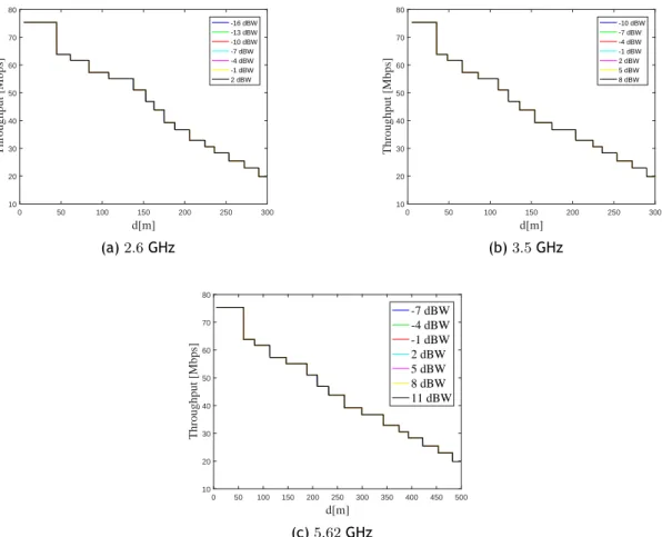
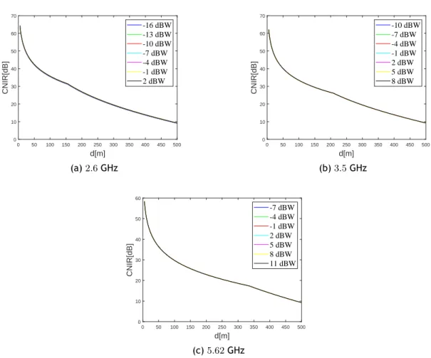
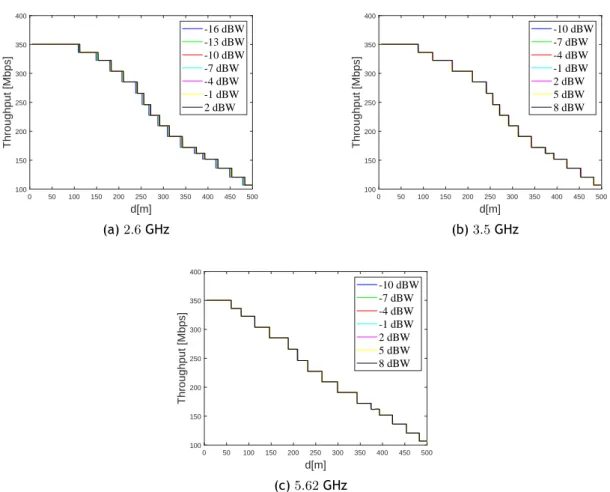
2.6 CNIR and Physical Throughput Evaluation . . . 33
2.7 Analytical Formulation of the Average CNIR . . . 48
2.8 Analytical Formulation Supported Throughput . . . 51
2.9 Cost/Revenue Optimization . . . 53
2.10 Summary and Conclusions . . . 58
3 Cellular Planning and Optimization with Carrier Aggregation 61 3.1 LTE-Sim Packet Level Simulator . . . 61
3.2 Carrier Aggregation in 3GPP . . . 64
3.3 Carrier Aggregation with LTE-Sim . . . 65
3.3.1 General Multi-band Scheduler . . . 67
3.3.2 Enhanced Multi-band Scheduler . . . 69
3.4 Simulations Results . . . 69
3.4.1 Packet Loss Ratio for Scenario 1 . . . 70
3.4.2 Delay for Scenario 1 . . . 71
3.4.3 Goodput for Scenario 1 . . . 72
3.4.4 Packet Loss Ratio for Scenario 2 . . . 78
3.4.5 Delay for Scenario 2 . . . 78
3.4.6 Goodput for Scenario 2 . . . 79
3.5 Conclusions . . . 79
4 Conclusions and Future Research 83 4.1 Conclusions . . . 83
4.2 Future activities . . . 84
References 87 A Further Results for 5G New Radio and LTE 95 A.1 Further Results for physical throughput in 5G New Radio . . . 95
A.2 3D view of the Mapping between MCS and Physical Throughput for Different Inter-ferer Positioning . . . 96
B Matlab code for 5G New Radio 107 C Analytical Formulation for the Average CNIR 113 D 4G Network with OpenLTE and srsLTE 123 D.1 srsLTE General Description . . . 123
List of Figures
1.1 Tentative timeline for 3GPP 5G . . . 3
1.2 Examples of NB-IoT deployment and typical required data rate . . . 7
1.3 Examples of NB-IoT deployment in downlink . . . 7
2.1 Resource grid in downlink . . . 12
2.2 Physical channel processing procedures . . . 13
2.3 Non-roaming 5G system architecture . . . 13
2.4 Illustration of PDSCH repetition and dynamic signaling of the number of PDSCH transmissions . . . 14
2.5 New Radio Frame Structure . . . 16
2.6 New Radio deployment scenarios . . . 17
2.7 New Radio frequency bands defined by Rel. 15 . . . 17
2.8 Scenario with k = 3, where first interference ring with six interferers are repre-sented . . . 20
2.9 Cell planning for k = 3 with distance calculated for the worst case scenario . . . 22
2.10 Scenario with k = 4, first interference ring and six interferers . . . . 24
2.11 Cell planning for k = 4 with distance calculated for the worst case scenario . . . 25
2.12 Positioning of interferes for the spectrum sharing scenario . . . 26
2.13 Positioning of interferes and representation of the respective cell radius . . . 27
2.14 Different CNIR values for different transmitter powers . . . 29
2.15 Different Physical throughput values for different transmitter powers in LTE . . . 30
2.16 Different CNIR values for different transmitter powers for 5G New Radio . . . 31
2.17 Different Physical throughput values for different transmitter powers in 5G New Radio . . . 32
2.18 Pathloss and received power . . . 32
2.19 CNIR and Physical throughput as a function of d for the No and East interferer scenario for k = 3 . . . . 34
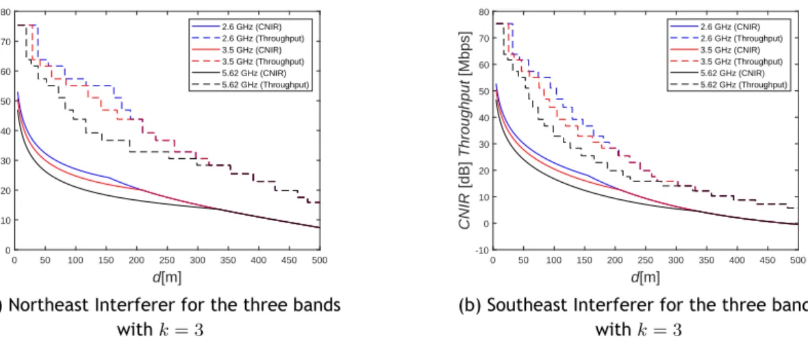
2.20 CNIR and Physical throughput as a function of d for the Northeast and Southeast interferer scenario for k = 3 . . . 35
2.21 CNIR and Physical throughput as a function of d for the No and East interferer scenario for k = 4 . . . . 35
2.22 CNIR and Physical throughput as a function of d for the Northeast and Southeast scenario for k = 4 . . . . 35
2.23 3D View of the PHY throughput mapped into MCSs with No Interferer at the 2.6 GHz band with k = 3 . . . 37 2.24 3D View of the PHY throughput mapped into MCSs with Northeast Interferer ate
the 2.6 GHz band with k = 3 . . . . 37 2.25 3D View of the PHY throughput mapped into MCSs with No Interferer at the 3.5
GHz band with k = 3 . . . 38 2.26 3D View of the PHY throughput mapped into MCSs with Northeast Interferer at the
3.5GHz band with k = 3 . . . . 38 2.27 3D View of the PHY throughput mapped into MCSs with No Interferer at the 5.62
GHz band with k = 3 . . . 39 2.28 3D View of the PHY throughput mapped into MCSs with Northeast Interferer at the
5.62GHz band with k = 3 . . . . 39 2.29 CNIR and Physical throughput as a function of d for the No and East interferer
scenario for k = 3 and bandwidth of 100 MHz . . . . 43 2.30 CNIR and Physical throughput as a function of d for the Northeast and Southeast
interferer scenario for k = 3 and bandwidth of 100 MHz . . . . 43 2.31 CNIR and Physical throughput as a function of d for the No and East interferer
scenario for k = 4 and bandwidth of 100 MHz . . . . 43 2.32 CNIR and Physical throughput as a function of d for the Northeast and Southeast
interferer scenario for k = 4 and bandwidth of 100 MHz . . . . 44 2.33 3D View of the PHY throughput mapped into MCSs with No Interferer at the 2.6
GHz band with k = 3 . . . 45 2.34 3D View of the PHY throughput mapped into MCSs with Northeast Interferer at the
2.6GHz band with k = 3 . . . . 46 2.35 3D View of the PHY throughput mapped into MCSs with No Interferer at the 3.5
GHz band with k = 3 . . . 46 2.36 3D View of the PHY throughput mapped into MCSs with Northeast Interferer at the
3.5GHz band with k = 3 . . . . 47 2.37 3D View of the PHY throughput mapped into MCSs with No Interferer at the 5.62
GHz band with k = 3 . . . 47 2.38 3D View of the PHY throughput mapped into MCSs with Northeast Interferer at the
5.62GHz band with k = 3 . . . . 48 2.39 Average SINR different values for different transmitter powers . . . 49 2.40 Comparison between Average SINR with different values for the transmitter power
2.41 Average SINR different values for different transmitter powers with 100MHz
band-width . . . 50
2.42 Comparison between Average SINR with different values for the transmitter power for the 2.6 GHz, 3.5 GHz and 5.62 GHz, and 100 MHz bandwidth . . . . 51
2.43 Areas of the coverage rings where a given value of PHY throughput for hexagonal has a transition . . . 51
2.44 Comparison of the supported throughput for k = 3 in the pico cellular scenario, for different positions of the interferer from MO #2 and for the case without interference with 20 MHz bandwidth . . . 52
2.45 Comparison of the supported throughput for k = 4 in the pico cellular scenario, for different positions of the interferer from MO #2 and for the case without interference with 20 MHz bandwidth . . . 52
2.46 Comparison of the supported throughput for k = 3 in the pico cellular scenario, for different positions of the interferer from MO #2 and for the case without interference with 1000 MHz bandwidth . . . 53
2.47 Comparison of the supported throughput for k = 4 in the pico cellular scenario, for different positions of the interferer from MO #2 and for the case without interference with 1000 MHz bandwidth . . . 53
2.48 Variation of CNIR and Physical throughput for dmax=1000 m . . . 56
2.49 Variation of supported throughput for Rmax=1000 m . . . 56
2.50 Revenue per cell for Rmax=1000 m . . . 57
2.51 Network cost/revenue per unit are per year as a function of R, for Rmax=1000 m 57 2.52 Profit per unit area per year as a function of R, Rmax=1000 m . . . 58
3.1 Protocol stack of LTE-Sim . . . 61
3.2 FDD Frame Structure . . . 63
3.3 TDD Frame Structure . . . 63
3.4 CA allocation examples in LTE/LTE-A . . . 65
3.5 Inter band carrier aggregation deployment scenario . . . 66
3.6 Inter band carrier aggregation deployment scenario with Small Cells . . . 67
3.7 Average cell PLR as a function of UEs for R=1000 m . . . 70
3.8 3D view of the average cell PLR for the three schedulers . . . 71
3.9 Average cell delay as a function of UEs for R=1000 m . . . 72
3.10 3D view of the average cell delay for the three schedulers . . . 73
3.11 Average cell supported goodput as a function of UEs for R=1000 m . . . 74
3.12 3D view of the average cell goodput for the three schedulers . . . 75
3.13 Average cell goodput for a threshold of 2% PLR . . . 76
3.16 3D representation of cell MCS for the 2.6 GHz carrier . . . 76
3.14 3D representation of the cell SINR for the 2.6 GHz carrier . . . 77
3.17 3D representation of cell MCS for the 800 MHz carrier . . . 77
3.18 Average cell PLR as a function of UEs for R=1000 m . . . 78
3.19 Average cell delay as a function of UEs for R=1000 m . . . 79
3.20 Average cell goodput as a function of UEs for R=1000 m . . . 80
A.1 3D View of the PHY throughput mapped into MCSs with No Interferer at the 2.6 GHz band with k = 4 . . . 96
A.2 3D View of the PHY throughput mapped into MCSs with Northeast Interferer at the 2.6GHz band with k = 4 . . . . 97
A.3 3D View of the PHY throughput mapped into MCSs with No Interferer at the 3.5 GHz band with k = 4 . . . 98
A.4 3D View of the PHY throughput mapped into MCSs with Northeast Interferer at the 3.5GHz band with k = 4 . . . . 99
A.5 3D View of the PHY throughput mapped into MCSs with No Interferer at the 5.62 GHz band with k = 4 . . . 99
A.6 3D View of the PHY throughput mapped into MCSs with Northeast Interferer at the 5.62GHz band with k = 4 . . . . 99
A.7 3D View of the PHY throughput mapped into MCSs with No Interferer at the 2.6 GHz band with k = 4 . . . 100
A.8 3D View of the PHY throughput mapped into MCSs with Northeast Interferer at the 2.6GHz band k = 4 . . . 100
A.9 3D View of the PHY throughput mapped into MCSs with No Interferer at the 3.5 GHz band with k = 4 . . . 100
A.10 3D View of the PHY throughput mapped into MCSs with Northeast Interferer at the 3.5GHz band with k = 4 . . . 101
A.11 3D View of the PHY throughput mapped into MCSs with No Interferer at the 5.62 GHz band with k = 4 . . . 101
A.12 3D View of the PHY throughput mapped into MCSs with Northeast Interferer at the 5.62GHz band with k = 4 . . . 101
A.13 3D View of the PHY throughput mapped into MCSs with East Interferer at the 2.6 GHz band with k = 3, bandwidth of 100 MHz and SCS 60 kHz . . . 102
A.14 3D View of the PHY throughput mapped into MCSs with South East Interferer at
the 2.6 GHz band with k = 3, bandwidth of 100 MHz and SCS 60 kHz . . . 102
A.15 3D View of the PHY throughput mapped into MCSs with East Interferer at the 2.6 GHz band with k = 4, bandwidth of 100 MHz and SCS 60 kHz . . . 102
A.16 3D View of the PHY throughput mapped into MCSs with South East Interferer at the 2.6 GHz band k = 4, bandwidth of 100 MHz and SCS 60 kHz . . . 103
A.17 3D View of the PHY throughput mapped into MCSs with East Interferer at the 3.5 GHz band with k = 3, bandwidth of 100 MHz and SCS 60 kHz . . . 103
A.18 3D View of the PHY throughput mapped into MCSs with South East Interferer at the 3.5 GHz band with k = 3, bandwidth of 100 MHz and SCS 60 kHz . . . 103
A.19 3D View of the PHY throughput mapped into MCSs with East Interferer at the 3.5 GHz band with k = 4, bandwidth of 100 MHz and SCS 60 kHz . . . 104
A.20 3D View of the PHY throughput mapped into MCSs with South East Interferer at the 3.5 GHz band with k = 4, bandwidth of 100 MHz and SCS 60 kHz . . . 104
A.21 3D View of the PHY throughput mapped into MCSs with East Interferer at the 5.62 GHz band with k = 3, bandwidth of 100 MHz and SCS 60 kHz . . . 104
A.22 3D View of the PHY throughput mapped into MCSs with South East Interferer at the 5.62 GHz band with k = 3, bandwidth of 100 MHz and SCS 60 kHz . . . 105
A.23 3D View of the PHY throughput mapped into MCSs with East Interferer at the 5.62 GHz band with k = 4, bandwidth of 100 MHz and SCS 60 kHz . . . 105
A.24 3D View of the PHY throughput mapped into MCSs with South East Interferer at the 5.62 GHz band with k = 4, bandwidth of 100 MHz and SCS 60 kHz . . . 105
C.1 Division of the Own cell for the first scenario . . . 115
C.2 Division of the Own cell for the second scenario . . . 115
C.3 Division of the cell to calculate integrals . . . 117
C.4 Division of the cell . . . 118
C.5 Division of the cell . . . 119
C.6 Division of the cell . . . 120
C.7 Division of the cell . . . 121
D.1 srsLTE labrary structure . . . 124
D.2 EPC at machine one . . . 126
D.3 eNODEB at machine one . . . 127
D.4 Connection with UE running on machine two . . . 127
D.6 LTE Test Network in mobile phone . . . 128 D.7 Plot of signal with srsGUI . . . 129
List of Tables
2.1 NR Frequency Bands . . . 18
2.2 Different transmitter powers considered for both frequencies . . . 28
2.3 Parameters considered . . . 33
2.4 Resource Block Allocation in LTE . . . 33
2.5 Mapping into Physical throughput for 20 MHz bandwidth. . . 34
2.6 Transmission bandwidth configurations for 5G NR . . . 40
2.7 TBS for 5G for Ninf o≤ 3824 . . . 41
2.8 NR UL Throughput for a bandwidth of 20 MHz and SCS of 30 kHz . . . 44
2.9 Assumptions for base station costs . . . 55
3.1 Uplink-downlink configurations for frame structure 2 . . . 64
A.1 NR UL maximum Throughput for a bandwidth of 30 MHz and subcarrier spacing of 30 kHz . . . 96
A.2 NR UL maximum Throughput for a bandwidth of 40 MHz and sucarrier spacing of 30 kHz . . . 97
A.3 NR UL maximum Throughput for a bandwidth of 100 MHz and sucarrier spacing of 30 kHz . . . 98
List of Acronyms
1G First Generation
3G Third Generation
4G Fourth Generation
5G Fifth Generation
3GPP Generation Partnership Project AMF Access Mobility Functions AMPS Advance Mobile Phone System
ARIB Association of Radio Industries and Businesses ATIS Alliance for Telecommunications Industry Solutions
BER Bit Error Rate
BMBS Basic Multi-Band Scheduler
BS Base Station
CA Carrier Aggregation
CBR Constant Bit Rate
CC Carrier Component
CCSA China Communications Standards Association CDMA Code Division Multiple Access
CNIR Carrier to Noise plus Interference Ratio
CoMP Coordinated Multipoint Transmission and Reception COST European Cooperation in Science and Technology
CP Cyclic Prefix
CP-OFDM Cyclic Prefix Orthogonal Frequency Division Multiplexing CQI Channel Quality Indicator
CSI Channel State Information
CSI-RS Channel State Information Reference Signal
CT Core Network and Terminals
DL Downlink
DM-RS Demodulation Reference Signal
DwPTS DL Pilot Time Slot
eICIC enhanced Inter-Cell Interference Coordination eLAA enhanced Licensed Assisted Access
EMBS Enhanced Multi Band Scheduler
eNB evolved Node B
EPC Evolved Packet Core
ePDCCH enhance Physical Downlink Control Channel
EPS Evolved Packet System
ETIS European Telecommunications Standards Institute E-UTRA Evolved Universal Terrestrial Radio Access
FDD Frequency Division Duplexing FDTD Finite-Difference Time-Domain
FR1 Frequency Range 1
FR2 Frequency Range 2
gNB Next Generation Node B
GMBS General Multi Band Scheduler
GP Guard Period
GSM Global System for Mobile Communications HetNets Heterogeneous Networks
IEEE Institute of Electrical and Electronics Engineers
IGP Integer Programing
IMT International Mobile Telecommunications
IoT Internet of Things
IP Internet Protocol
IPv4 Internet Protocol version 4 IPv6 Internet Protocol version 6
IT Instituto de Telecomunicações
ITU International Telecommunication Union
LBR Low-Power Border Router
LTE Long Term Evolution
LTE-A Long Term Evolution -Advanced LTE-U Long Term Evolution -Unlicensed
MCN Macro Cell Network
MCS Modulation Code Scheme
MIMO Multiple Input Multiple Output
M-LWDF Modified-Largest Weighted Delay First
mmWave Millimeter Wave
NF Network Functions
NMT Nordic Mobile Telephone
NR New Radio
NTT Nippon Telephone and Telegraph
OFDM Orthogonal Frequency Division Multiplexing OFDMA Orthogonal Frequency Division Multiple Access PDCCH Physical Downlink Control Channel
PDU Protocol Data Unit
PDSCH Physical Downlink Shared Channel
PF Profit Function
PLMN Public Land Mobile Network
PLR Packet Loss Ratio
PUCCH Physical Uplink Control Channel PUSCH Physical Uplink Shared Channel
QoS Quality of Service
RAN Radio Access Network
RAT inter-Radio Access Technology
Rel Release
RF Radio Frequency
RS Reference Signal
SA Systems Aspects
SSB Single Band Side
SSC Session and Service Continuity
SC Small Cell
SCS Sub Carrier Spacing
SINR Signal to Interference and Noise Ratio
SMF Section Management Function
S-NSSAI Single - Network Slice Selection Assistance Information
SRS Sounding Reference Signal
TBS Transport Block Size
TDD Time Division Duplexing
TDMA Time Division Multiple Access
TNL Transport Network Layer
TSDS Telecommunications Standards Development Society TTA Telecommunications Technology Association
TTC Telecommunication Technology Committee
UE User Equipment
UL Uplink
UMTS Universal Terrestrial Mobile System
UpPTS UL Pilot Time Slot
USIM Universal Subscriber Identity Module
VoIP Voice over IP
VPLMN Visited Home Public Land Mobile Network WLAN Wireless Local Area Network
Chapter 1
Introduction
1.1
Motivation
The exponential growth of machine-to-machine communications and the continuous develop-ment of bandwidth-demanding applications have created a scenario where the cellular networks are approaching their edge [1]. This scenario has created in increasing interest in researches about the deployment of Small Cell (SC) access points to ensure extended coverage and link budget. In this scenario of Heterogeneous Networks (HetNets) there is a variety of small range cells that underlays the Macro Cell Network (MCN) and this approach can enhance coverage and spatial reuse allowing cellular systems to deliver higher data rates preserving mobility and connectivity. Carrier Aggregation (CA) has been adopted for operator to address the growing challenges surrounding high data demand in mobile communications and it can be deployed in both Frequency-Division Duplexing (FDD) and Time-Division Duplexing (TDD) frame structure al-lowing for the increase of transmission bandwidth over those that can be supported by a single channel or carrier. CA plays a key role in the Long Term Evolution Advanced (LTE-A) meeting requirements for large transmissions width (40 MHz-100 MHz) and high peak data rates of 500 Mbps in the uplink (UL) and 1 Gbps in the downlink (DL) [2]. Also, in 2018 the 3rd Generation
Partnership Project (3GPP) finished the technical specifications for 5G New Radio (NR), and the first commercial 5G networks started to operate in the first semester of 2019. The technol-ogy of 5G NR will allow for significantly more faster wireless communication and will greatly improve the subscriber’s experiences, by delivering much higher data rates in both uplink and downlink direction. New Radio is expected to make extensive use of CA and SC deployment as well as Multiple Input Multiple Output (MIMO) alongside other technologies, what brings further importance to the study of SCs deployment scenarios. All this context motivates the research presented in this master thesis, where one CA and SCs deployment are investigated through ana-lytical formulations and simulations. The technical specifications 5G are also explored as a first step towards the expansion of the research performed by IT in the direction of the upcoming technology.
1.2
State of the Art
1.2.1
Evolution of Mobile Communications
In the study of the evolution of mobile communications, the cellular wireless generation (G)is a term used to characterize the changes in the services provided by the operators and incorpo-ration of new technologies, such as new frequency bands or frame structures [3]. In this sense, one can sumarize the steps in this evolution process as follows:
• First Generation (1G) characterized by the use of analog networks;
• Second Generation (2G) with the introduction of digital multiple access technologies; • Third Generation (3G) with support to multimedia services;
• Fourth Generation (4G);
• Fifth Generation (5G) New Radio.
The first cellular system of what would latter be known as 1G began its operation in 1979 in Tokyo, Japan, deployed by Nippon Telephone and Telegraph (NTT). It was characterized by the use of analog communication systems to transmit voice data, using Frequency-Division Multiple Access (FDMA) to modulate signals in frequencies of about 150 MHz [4]. Several 1G standards were adopted across the globe such as the Nordic Mobile Telephone (NMT) for the Nordic coun-tries and the Advanced Mobile Phone System (AMPS) in the United States which adopted a 40 MHz bandwidth and 800 to 900 MHz as operating frequencies with a reuse pattern (k) of 7. The second generation, or 2G was introduced in the late 1980s bringing with it new technologies such as Time Division Multiple Access (TDMA) and Code Division Multiple Access (CDMA) [5]. This new generation brought a series of improvements when compared to 1G, such as better data services and higher spectral efficiency, and some operators also offered Short Message Service (SMS). The first 2G networks based on the Global System for Mobile Communications (GSM) were launched in Finland in 1991.
The third generation had its first commercially available network deployed in Japan by NTT in 2001 [6]. This generation offers a wide range of services that the covers the possibilities of the previous generations but also improves upon it by offering more advanced resources such as video calls and broadband wireless data, all with improved spectral efficiency. The development of the 3G was not uniform, varying according to the region [7] what gave birth to several standards such as Universal Terrestrial Mobile System (UMTS) in Europe [8] or the CDMA2000, which is the American variety of 3G [9].
The first tests of what would be known as 4G were conducted in Tokyo, Japan in 2005 where field trials demonstrated that the new technology was able to achieve speeds up to 1 Gbps in the downlink direction. 4G improves upon the technology of 3G offering high quality audio and video streams
The initial specifications for the fifth generation of cellular communications, or 5G NR were completed by the the 3GPP in June of 2018, starting the non-standalone phase of the tech-nology, where it is expected to work alongside the existing 4G/LTE infrastructure, offering retro-compatibility with existing services [10]. By the time this work is being written, the first commercial 5G networks are already operating in some regions of the world, namely South Korea [11], United States [12] and Uruguay [13].
1.2.2
3GPP
The 3rd Generation Partnership Project covers cellular telecommunications network technolo-gies that include radio access, core transport network and service capabilities [14]. This project includes telecommunications organizations (ARIB, ATIS CCSA, ETSI, TSDSI, TTA, TTC) that coop-erate in the development of standards and specifications for the underlying technologies and it is composed of three technical specifications groups: Radio Access Network (RAN), Services and Systems Aspects (SA) and Core Network and Terminals (CT).
Rel.14 of 3GPP started the work on critical enhancements such as LTE support for V2x services, enhanced Licensed Assisted Access (eLAA) and 4 band carrier aggregation while Rel.15 brought the first 5G specifications and continued the maturing process of LTE-Advanced Pro. The pro-posed 3GPP time line for 5G in Figure 2.7.
Rel.10 introduced the first specifications for LTE-Advanced to meet International Telecommuni-cation Union (ITU)/International Mobile TelecommuniTelecommuni-cations (IMT)-Advance requirements, such as high speed higher achievable speeds to UEs compared to the specifications of Rel.8. This release also introduced some key features that would be further explored in the following re-leases, such as:
• Use of 8x8 MIMO communications in DL and 4x4 MIMO in the UL direction [16];
• The introduction of CA to allow the use of the fragmented spectrum inside the same fre-quency band or across different bands, what allows for an increase in throughput. LTE-Advanced allows the use of bandwidths up to 100 MHz using up to five CCs with the possi-bility of aggregating contiguous and non contiguous carriers [17];
• As Rel.10 brought the first specifications for the design of HetNets, it also included the Inhenced Inter-Cell Interference Coordination (eICIC) to deal with interference is these networks;
• This release first proposed the use of relay nodes as a resource to extend tho coverage area of a evolved NodeB (eNB), with the relays usually being low-power eNBs.
With the introduction of LTE-Advanced, Rel.11 brought some important enhancements to the standard previously established. For example, CA was further enhance with the introduction of non contiguous intra-band CA, multiple timing advances in the UL communication. It also introduced mechanism to allow a UE to reduce energy consumption by informing the network when it needs to run in battery saving mode, mainly due to data consumption by applications and process running in background. Other key features introduce by Rel.11 are:
• Network based positioning;
• Coordinated Multipoint Transmission and Reception (CoMP); • Enhance Physical Downlink Control Channel (ePDCCH) [18].
For Rel.12, enhancements to CA were brought with the possibility of applying CA between co-located TDD and FDD carriers. Also, integration of LTE and Wifi was introduced, to allow operator to have more control in aspects related to traffic control.
Rel.15 phase 1 of 3GPP corresponds to NR phase 1, while Rel.16 will cover the second phase for this technology. Even though the set of frequencies for 5G NR is firmly established, there is a convergence in use and other bands, such as 24.25 GHz and 33.4 GHz are being studied for use in this technology. The technology involved in the development of the 5G NR is expected to make extensive use Multiple Input Multiple Output (MIMO) communications with which is possible to
achieve up to 2 Gbps of DL speed, as shown in test scenarios [19]. Also, Rel.15 lists a set of technologies related to 5G NR:
• LTE-U/LAA ; • Multifire;
• LTE-Wireless Local Area Network (WLAN) aggregations; • Citizen Broadband Radio Service / Licensed Shared Access;
The development of 5G standard was divided in two phase i.e., NR phase 1 in Rel.15 and NR phase 2 in Rel.16. Even though in NR phase 1 there is a series of common elements between LTE and NR, the approach proposed by 3GPP was established to allow the use o existing hardware by considering a non-standalone version in which the LTE core is still present while in the standalone version NR core will work independently from LTE [20].
1.2.3
Heterogeneous Networks
One can define Heterogeneous Network as a network composed of a mix of low-power nodes and macrocells where some devices may be configured with directives of restrict access while others may lack a wired connections structures [21]. The study of cellular HetNets have become of paramount importance to researches over the last few decades, especially when one considers the exponential growth of mobile subscribers, and the uneven distribution of spectrum as well as its increasing scarcity, what makes mobile operators look for solutions to better use the available spectrum, usually deploying a series of devices with different transmit power, coverage or capacity, to ensure the quality of communication.
In the context of LTE broadband network deployment, one usually has scenarios of heavily dense urban areas or very remote areas, where a diversity of frequency bands is employed, with dif-ferent propagation characteristics, alongside an accentuated heterogeneity in terms of devices [22].
One common element in HetNets is the Small Cell which is deployed with the aim of increas-ing the capacity of a network per unit of area offloadincreas-ing the macrocells and improvincreas-ing indoor coverage and cell-edge user performance. SCs are classified as follows [23]:
• Microcells, also known as micro Base Stations (BSs) or serving microcells, usually have the same interface as a typical BS, but operate at a much lower transmit power. They are most commonly operator-deployed and one of its most common applications is to serve as outdoors hotspots, with its coverage usually limited up to 1 mile and controlled by its transmit power.
• Picocells are low-power SCs, usually operator-installed and have the same the same back-haul features of the BS, but operate at a much smaller transmitter power, usually around (30 dBm) [24], with a cell radius ranging from 100 to less than 299 m. This cells can be equipped with omnidirectional antennas or with a different directionality, offering cover-age up to 100 users.
• Femtocells also kwon as home base stations, are small low-power BSs which are usually consumer-deployed [25], commonly connected to their own wired back-haul, being des-ignated as Home evolved NodeB (HeNB) in LTE. This cells can be deployed indoors or out-doors, but the first option is usually the most common.
1.2.4
Narrowband IoT
NB-IoT was first introduced by 3GPP in Rel.13 [26] starting the work to ensure wide-are coverage within the context of the Internet of Things(IoT). The idea behind this release was to first address some of the main challenges found in the deployment of IoT-based use cases, such as:
• Battery life time;
• Deployments with massive number of devices;
• Flexibility;
• Mobility;
• Significant coverage extension.
The technology proposed for NB IoT, even though not completely backwards compatible with previous releases, makes extensive use of LTE-based technologies and standardizations. It employs downlink Orthogonal Frequency-Division Multiple-Access (OFDMA) alongside the same channel coding, rate matching, and interleaving [26]. One of the main characteristics proposed by 3GPP for NB-IoT is that it uses narrow bandwidth, what makes it possible to re-farm chunks of available spectrum from other technologies. It also employs the support to repetition of signals, make it possible to boost signals from low-power devices, thus reducing the levels of Packet Loss Ratio (PLR) [27]. Figure 1.2 shows some of the possible applications of NB-IoT, which are usually common to classical IoT devices, while 1.3 shows some applications deployment scenarios in the DL direction.
Figure 1.2: Examples of NB-IoT deployment and typical required data rate, adapted from [26]
Figure 1.3: Examples of NB-IoT deployment in downlink, adapted from [26]
1.3
Objectives and Approach
This MSc dissertation proposes the study of carrier Carrier Aggregation evaluating scenarios with and without Small Cells deployment to study the behavior of the of mobile networks under different parameters such as cell radius, number of User Equipment (UE) and interferers.The proposal is to make use of the LTE-Sim packet level simulator and the packet schedulers previ-ously developed by researchers from the Instituto de Telecomunicações-Covilhã to investigate the system´s capacity by considering the 2.6 GHz and 800 MHz frequency bands, and also to construct the framework necessary to allow the deployment of Small Cells in different locations and with different radius. To allow a comparative analysis of the results obtained, the frame-work used also performs the simulation of scenarios without CA, which can be compared with results from the scenarios that consider aggregation with and without SCs. Another objective of
this dissertation is to address spectrum sharing at the SC layer of the HetNet. Spectrum sharing assumes that two or more mobile operators/carriers have dedicated spectrum for macro cellu-lar layer while SCs will use exclusive shared spectrum (by paying a fee) or share the access to non-licensed spectrum in an opportunist manner. To achieve this goal, a analytical formulation is used considering different assumptions (“cases”) for the sharing scenario in the SC layer i.e., no sharing case scenario, where operators use the same frequency band or sharing with inter-ferers positioned at different geographical locations. In this context, one considers a mapping between Modulation Code Schemes (MCSs) and minimum CNIR to obtain the physical throughput following the specifications of 3GPP to LTE networks. Supported throughput and average Carrier to Noise plus Interference Ratio (CNIR) are also computed by considering different cell radius and distances between Base Station and User Equipment. One also considers the specifications of 5G New Radio to compute the metrics proposed for studying, by updating the Matlab code while considering a maximum modulation order of six.
1.4
Contributions
The main contributions of this MSc dissertation are the analytical computation of the average Carrier Plus Noise Interference Ration (CNIR) and physical and supported throughput under the technical specifications of LTE and 5G New Radio, considering the two slope propagation model and Small Cells deployment, for the Ultra High Frequency/Super High Frequency (UHF/SHF), presented in chapter 2. This study follows the research on Small Cells deployment from Insituto de Telecomunicações - Covilhã.
Another fundamental contribution is the study of Carrier Aggregation with the LTE-Sim packet level simulator and the implementation of Aggregation with Small Cells, give contributions to the research started at the Instituto de Telecomunicações. The results of this research are presented in Chapter 3, where one evaluates the system´s capacity under several metrics, such as PLR, goodput, delay and Signal plus Noise Signal-to-Interference-plus-Noise Ratio (SINR). The contributions of this work have already been presented in the following venues:
• One paper accepted for publications under the title ”Techno-Economic Trade-off of Small Cell 5G Networks”, to be presented in the 11thConference on Telecommunications
(Con-ftele 2019);
• Two Temporary Documents T D(19)10063 and T D(19)10065 in the 10thMC meeting and 10th
technical meeting of the COST CA 15104 held in Oulu, Finland from 27 to 29 of May 2019. Also, in the context of the research carried out by the member within IT-Covilhã team, the
development of energy efficient routing protocols has been addressed for applications on IoT scenarios. This research topic has been presented on the following venues:
• One paper accepted for publication under the title ”Performance Evaluation of Source Routing Minimum Cost Forwarding Protocol over 6TiSCH Applied to the OpenMote-B Plat-form”, in proceeding of The Urb-IoT 2018 - 3rdEAI International Conference on IoT in Urban
Space, Guimarães, Portugal, Nov. 2018;
• One paper accepted for publications under the title ”Source Routing Minimum Cost For-warding Protocol over 6TiSCH Applied to the OpenMote-B Platform”, to be presented in the 2019 IEEE 30thAnnual International Symposium on Personal, Indoor and Mobile Radio
Communications (PIMRC), Istanbul, Turkey, Sep. 2019;
• One Temporary Documents T D(19)09082 in the 9thMC meeting and 9thtechnical meeting
of the COST CA 15104 held in Dublin, Ireland, 16 - 18 of Jan 2019;
• One Temporary Documents T D(18)07052 in the 8thMC meeting and 8thtechnical meeting
of the COST CA 15104 held in Cartagena, Spain, May 16 - Jun. 1 of 2019.
1.5
Outline of the Dissertation
The first part of this master thesis gave a brief state of the art covering topics such as the evolution of mobile communications, the Third Generations Partnership Project and the contri-butions of its technical releases to the standardization of mobile technologies, Heterogeneous Networks, Carrier Aggregation and Small Cells.
Then, in chapter 2 a scenario for spectrum sharing is studied, making use of a analytical for-mulation to evaluate physical and supportable throughput as well as average Carrier Plus Noise Interference Ration by considering a deployment case based in Small Cells with a central cell, 6 co-channel cells, one cell from a different mobile operator and and a central cell.For the study presented in chapter two one considers the technical specifications of LTE and 5G New Radio, evaluating the system´s capacity by considering different cell radii and User Equipment distances. A cost/revenue analysis is also presented in chapter two, where the values obtained for the supported throughput obtained via the analytical formulation are used to estimate the economic tradeoff of Small Cells deployment.
In chapter 3 the LTE-Sim packet level simulator is used to implement and evaluate Carrier Ag-gregation considering deployment scenarios with and without Small Cells.One considers two different frequency bands and the system´s capacity is evaluated in terms of goodput, PLR, delay, and Signal plus Interference noise ratio.
Finally, chapter 4 draws conclusions to the work, with a brief overview of the results obtained and suggestions for future work. In appendices A, B, and C, further results are presented for the analytical formulation developed in chapter 2, as well as the code used with 5G New Radio and the analytical formulation for the average CNIR . Appendix D describes the work performed on the implementation of a 4G network with OpenLTE/srsLTE.
Chapter 2
Cellular Radio and Network Optimization:
Analytical Study
2.1
General Aspects of the Long Term Evolution
The Long Term Evolution is the radio interface standardized by 3GPP and had its first spec-ification brought by Rel.8, offering support for FDD and TDD. It was first proposed to offer a framework for communication with delays lower than 5 ms and possibilities for data rates achieving peaks of 300 Mbps [28].
Since its first release, LTE underwent a series of changes provided by the new releases of 3GPP with the aim of improving the technology to match the growing number of mobile subscribers, heterogeneity of mobile networks and demand for higher data rates and quality of service. New paradigms have been incorporated, such as the introduction of NB-IoT [29], the exploration of unlicensed spectrum [30] or the use of Unnamed Aerial Vehicles (UAVs) [31]. LTE has now reached Rel.15, where not only 5G New Radio had its first complete standardization, but improvements were also introduced to allow enhancements in network capacity mainly aiming at ensuring backwards compatibility of the existing infrastructure and new the technologies proposed by NR [32].
2.1.1
Downlink Physical Channels and Physical Layer Procedures
The modulation scheme adopted in LTE is based on the use Orthogonal Frequency Division Mul-tiplexing (OFDM) and it was first chosen due to its robustness against the effects of multi-path fading. It is also capable of performing multiplexing through the use of OFDMA offering a set of available bandwidths that goes from 1.4 MHz to 20 MHz. In the DL direction, the physical channels can transport information that are originated at higher layers or physical signals that are transmitted for the use of the physical layer.
An important element in LTE is the Physical Resource Block (PRB) and its allocation is handled by a scheduling algorithm, usually managed by the eNodeB in a network. Each LTE frame is constructed to have a duration of 10 ms and it is usually divided in 10 sub-frames of 1 ms each containing 2 slots with a length of 0.5 ms in the time domain. The number of resource blocks assigned to each slot depends on the operative bandwidth of the channel, e.g., 100 resource
blocks for a bandwidth of 20 MHz. Each resource block will be composed of 12 sub-carriers corresponding to each OFDM symbol, and the total number of OFDM symbols may be 7 for a normal cyclic prefix OFDM or 6 in long prefix. Figure 2.1, summarizes the formation of resource grids in the DL direction, where a resource element is the smallest possible unit for assignment of resources.
Figure 2.1: Resource grid in downlink, adapted from [33]
In cases when transmissions are based in more than one physical channel, the processing of the physical channel is performed according to the following 6 steps [33], which are summarized above and illustrated in figure 2.2.
• The first step consists in the scrambling of the code bits in each code word to be trans-mitted;
• In the second step, scrambled bits are modulated to produce complex values;
• In the third step, the complex values are mapped to one or more transmission layers; • Complex-valued symbols are then precoded in the fourth step, for transmission over the
antenna ports;
• In step five, the complex modulated values are mapped to resource elements, for each antenna port;
• Finally, in step 6, time-domain complex-valued OFDM signals are generated for each an-tenna port.
Figure 2.2: Physical channel processing procedures, adapted from [33]
2.2
5G New Radio Physical Layer
The general description of 5G NR given by Rel.15 allows for the deployment of a complete commercial network with a service based architecture employing the concept of modularity [34], where the elements of the architecture are called Network Functions (NFs) and offer their services via a common framework, as shown in figure 2.3.
The system presented above defines Access Mobility Functions (AMF) and Session Management Functions (SMF) that operate separately to ensure the modularity of the architecture. The tech-nology of 5G NR in terms of connectivity allows for services based on Protocol Data Unit (PDU) sessions of various types, such as Internet Protocol (IP) versions 4 (IPv4), and 6 (IPv6), Ethernet and Unstructured. To ensure the capability of providing IP addresses, the system provides the traditional Session and Service Continuity (SSC) and also brings new modules such as SSC mode 3. In this context, Quality of Service (QoS) is approached on a flow based framework, with the options of having QoS without signaling, based on standardized packet marking, or QoS signal-ing based, for more flexibility [36]. It also provides congestion and overload control, control plane load control, Transport Network Layer (TNL), AMF load balancing, SMF and AMF overload control.
In NR, UE’s accesses attempts to the network are categorized into access categories, via unified Access Control. This feature gives the network the possibility of restricting accesses with poli-cies based on categories. Furthermore, the technology allows for congestion control by means of DNN, Single - Network Slice Selection Assistance Information (S-NSSAI) and mobility manage-ment. Also, configurations into the Universal Subscriber Identity Module (USIM) card of a UE can be used to provide a list of preferred Public Land Mobile Network (PLMN) via access technology combinations monitoring roaming in a Visited Home Public Land Mobile Network (VPLMN). NR is expected to make intensive use of MIMO communications in the different scenarios of deployment. Rel.15 specifies the support for multi-layer transmissions with the possibility of a maximum of four transmission layers in the UL direction and eight transmission layers in the DL directions. In this sense, scheduling procedures in NR consider the use of large numbers of multi-user MIMO users with Physical Downlink Shared Channel (PDSCH)/Physical Uplink Shared Channel (PUSCH) demodulation, and DL Channel State Information (CSI) acquisition supporting CSI Reference Signal (CSI-RS), Sounding RS (SRS), and Demodulation RS (DM-RS). Figure 2.4 shows the structure of PDSCH repetition and dynamic signaling adopted by NR.
Figure 2.4: Illustration of PDSCH repetition and dynamic signaling of the number of PDSCH transmissions, adapted from [37]
2.2.1
NR Physical Layer Procedures
Bean management in the DL direction is performed by means of Single Band Side (SSB) and Chan-nel State Information Reference Signal (CSI-RS), while SRS is used in the uplink direction where related procedures can be enhanced by the use of sweeping spatial filters at transmitter. UEs inside a network receive information about bean alignment on transmission beans for Physical Downlink Control Channel (PDCCH), Physical Uplink Control Channel (PUCCH) and PDSCH so that a UE can be able to identify and misalignment, transmitting information to inform the Next Gen-eration nodeB (gNB). It also allows for the recovery of bean failure when misalignment between transmission/receptions beans occurs.
NR offers support codebooks for UL communications that allow for the deployment of networks with different implementations of transmitter phase coherence. Also, for the UL direction, there is possibility of employing non-codebook based transmissions with the gNB performing the selections of the appropriated transmissions layer by means of SRS resources transmitted by the UE.
5G NR is expected to allow for backward compatibly with LTE/LTE-A in the non-standalone phase, with the cells of both technologies offering different or the same coverage. Within NR deployment scenarios, it is possible to have a LTE/LTE-A eNB as a master node, offering an anchor carrier that can be boosted by a NR gNB, with data flow aggregated by the Evolved Packet Core (EPC) [36]. On the other hand, it is also possible to have a NR gNB as the master node, offering wireless services via the next generation core. In the latter case, an enhanced LTE (eLTE) eNB offers a booster carrier to the anchor node.
eLTE eNB can also be the master node in a standalone operation to offer wireless services. In this scenario, the eLTE eNB can work via the next generation core or have a collocated NR gNB to provide booster carriers. Finally, inter-Radio Access Technology (RAT) is expected to be applied in scenarios where the NR gNB is connected to the next generation core and the LTE-A eNB is connected to the EPC, to ensure handover between eNB and gNB. The possible deployment scenarios for 5G NR are presented in figure 3.4.
The numerologies of NR consider a Sub Carrier Spacing (SCS) that can assume values configured as subsets or super-sets of a 15 kHz spacing, with the possibility of inserting multiple cyclic prefix lengths for each sub-carrier. As the carrier frequencies of NR are higher than those of LTE/LTE-Advanced, one can expect these carrier frequencies to be more susceptible to the Doppler effect, but this effect can be mitigated by the employment of larger SCS.
2.2.2
NR Frame Structure
As define by 3GPP Rel.15, the sub-frames of NR are composed of slots that comprise 14 OFDM symbols, with lengths of 1 ms and 15 kHz of SCS. NR also adopts mini-slots that can carry control signal and mark the beginning or end of OFDM symbols. This structure allows for the possibility of allocating small packet sizes and also brings the possibility of immediately allocating resources for urgent data arrivals. Figure 2.5 shows the basic frame structure of 5G NR.
Figure 2.5: New Radio Frame Structure, adapted from [38]
It is possible to see from the representation in figure 2.5 that, when SCS is larger than 15 kHz, some of the OFDM symbols and CP lengths should be to the duration of one 15 kHz symbol duration, including CP length. Rel.15 of 3GPP has established two sets of frequency ranges identified as Frequency Range 1 (FR1) and Frequency Range 2 (FR2) as shown in figure 2.7. FR1 comprises the sub-6GHz frequency range (450-6000 MHz) while FR2 is the mmWave range (24250-52600 MHz).
Table 2.1 shows the complete set of frequency bands defined by Rel.15 that where identified considering marketing demand and also to allow the possibility of re-farming LTE bands. Consid-ering this aspects, it is possible to identify, from 2.1 bands corresponding to their equivalents in LTE, such as band n7, while the bands in FR1 are new frequency bands introduced in 5G NR.
2.3
Propagation Model
The recent developments in wireless communications and the constant search for more efficient and reliable ways to ensure data delivery followed by the increasing number of mobile subscriber all around the world has led, in the past few years to the development of several propagation
Figure 2.6: New Radio deployment scenarios, adapted from [39]
Figure 2.7: New Radio frequency bands defined by Rel. 15, adapted from [40]
models for applications in cellular mobile communications [41]. This models are of paramount importance to the correct characterization of the environment, system design, planning and testing [42].
Choosing a propagation model depends on several factors, such as environmental characteristics, type of application, frequencies to be applied, distances to be considered, and the computa-tional cost of the chosen model.The large-scale propagation models are usually classified in four groups [43]:
• Empirical models; • Semi-empirical models; • Deterministic models;
Table 2.1: NR Frequency Bands, adapted from [40]
NR operating band Uplink(UL) operating band Downlink(UL) operating band Duplex mode
n1 1920 MHz – 1980 MHz 2110 MHz – 2170 MHz FDD n2 1850 MHz – 1910 MHz 1930 MHz – 1990 MHz FDD n3 1710 MHz – 1785 MHz 1805 MHz – 1880 MHz FDD n5 824 MHz – 849 MHz 869 MHz – 894 MHz FDD n7 2500 MHz – 2570 MHz 2620 MHz – 2690 MHz FDD n8 880 MHz – 915 MHz 925 MHz – 960 MHz FDD n12 699 MHz – 716 MHz 729 MHz – 746 MHz FDD n20 832 MHz – 862 MHz 791 MHz – 821 MHz FDD n25 1850 MHz – 1915 MHz 1930 MHz – 1995 MHz FDD n28 703 MHz – 748 MHz 758 MHz – 803 MHz FDD n34 2010 MHz – 2025 MHz 2010 MHz – 2025 MHz TDD n38 2570 MHz – 2620 MHz 2570 MHz – 2620 MHz TDD n39 1880 MHz – 1920 MHz 1880 MHz – 1920 MHz TDD n40 2300 MHz – 2400 MHz 2300 MHz – 2400 MHz TDD n41 2496 MHz – 2690 MHz 2496 MHz – 2690 MHz TDD n51 1427 MHz – 1432 MHz 1427 MHz – 1432 MHz TDD n66 1710 MHz – 1780 MHz 2110 MHz – 2200 MHz FDD n70 1695 MHz – 1710 MHz 1995 MHz – 2020 MHz FDD n71 663 MHz – 698 MHz 617 MHz – 652 MHz FDD n75 N/A 1432 MHz – 1517 MHz SDL n76 N/A 1427 MHz – 1432 MHz SDL n77 3300 MHz – 4200 MHz 3300 MHz – 4200 MHz TDD n78 3300 MHz – 3800 MHz 3300 MHz – 3800 MHz TDD n79 4400 MHz – 5000 MHz 4400 MHz – 5000 MHz TDD n80 1710 MHz – 1785 MHz N/A SUL n81 880 MHz – 915 MHz N/A SUL n82 832 MHz – 862 MHz N/A SUL n83 703 MHz – 748 MHz N/A SUL n84 1920 MHz – 1980 MHz N/A SUL n86 1710 MHz – 1780MHz N/A SUL n257 26500 MHz – 29500 MHz 26500 MHz – 29500 MHz TDD n258 24250 MHz – 27500 MHz 24250 MHz – 27500 MHz TDD n260 37000 MHz – 40000 MHz 37000 MHz – 40000 MHz TDD n261 27500 MHz – 28350 MHz 27500 MHz – 28350 MHz TDD • Hybrid models.
Empirical models are based on measurements which make them very specific to each type of application. They are also usually simple, with a smaller number of parameters when compared to other models, what makes this models less complex in term of computational cost. One of the most widely none empirical models is the COST 231 One Slope Model, described by equation 2.1:
P L = L0+ 10nlog(d) (2.1)
characterizes the general losses of the system and n is the path loss exponent.
While empirical models offer less computational cost, they are also less accurate when com-pared to other models. Semi-empirical models, on the other hand offer a trade-off between complexity and accuracy offering higher accuracy by introducing deterministic factors. Some examples of this type of propagation models are the COST 231 Walfisch-Ikegami model [44], the Multiwall model [45], and COST 231 [46] penetration model.
Deterministic models also take into account information specific to the site of application, but are usually less complex in terms of computational cost when compared to empirical models. They are usually subdivided into finite-difference time-domain models (FDTD) and geometry models.
The work developed in this thesis considers the propagation model presented in [47] which is a two slope model applied to Urban Micro (UMi) scenarios line of sight (LoS). The UmiLoS model considers a range d≥ 10 but it is also analyzed for smaller distances in this work.
Considering the existence of a break point distance d′BP described by equation 2.2, the pathloss
is given by equation 2.3:
d′BP =
4h′U Eh′BSf
c (2.2)
P L1 = 22 log10(d) + 28 + 20 log10(f ), when d≤ d′BP
P L2 = 40 log10(d) + 7.8− 18 log10(h′BS)− 18 log10(h′U E) + 2 log10(f ), when d > d′BP (2.3)
where c = 3.0∗ 108m/s is the propagation velocity in free space and f is the frequency in GHz.
hBS is the height of the base station in m, hU E is the height of the User Equipment in m, (hBS
and both parameters can be obtained following the relation h′U E= hU E− 1 and h′BS= hBS− 1
and hU E). For 2.6 GHz the breakpoint distance is 156 m and for 3.5 GHz is 210 m and for 5.85
GHz is 351 m.
The Friis equation 2.4 is used to compute the received power at the receiver:
PR= PE+ GE+ GR− P L (2.4)
where PR is the received power given in dBW, PE is the transmitter power given in dBW, GE
pathloss values given in dB.
2.4
Cellular Topology and Spectrum Sharing
5G NR networks are expected to provide very high data rates while ensuring the delivery of QoS, what will cause a significant increase in the demand for spectrum [48]. In this context, SCs deployment with spectrum sharing is presented as a solution offering the possibility of of-floading the traffic from the macro cell and also to ensure coverage [49]. The exploration of LTE-Unlicensed is also of particular interest for the planning process and to perform experimen-tal research.
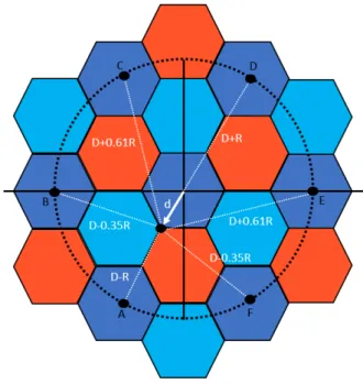
This section gives a general description of the chosen cellular topology. Considering a hexagonal cellular hexagonal topology, as the one shown in figure 2.8, with a frequency reuse distance,
D =√3kR, where R is the radius of the hexagonal cell, the users will be moving in the direction of the cell’s edge 5 ≤ d ≤ R, starting from the cell´s center. The carrier-to-noise ratio, C
I, is given by: C I = 1 2(rcc + 1)−γ+ 2(rcc)−γ+ 2(rcc− 1)−γ (2.5)
Figure 2.8: Scenario with k = 3, where first interference ring with six interferers are represented In a scenario considering shared spectrum, coordinates of UE for the worst case scenario are (−R2 ;−√23R), while for a general scenario are (−d2 ;−√23d). With this information, one can obtain the distance between UEs and interferes as follows:
d =√(x− x0)2+ (y− y0)2 (2.6)
The first case analized in this section considers one interference ring, and so one has six inter-feres (SC eNBA, SC eNBB, SC eNBC, SC eNBD, SC eNBE, SC eNBF) as shown in figure 2.8. We also consider a reuse pattern k = 3. The distances for the worst case scenario can be summarized as follows:
• For the interferent SC eNBA the coordinates are (−3R2 ;−3√3R 2 );
• For the interferent SC eNBB the coordinates are (−3R; 0); • For the interferent SC eNBC the coordinates are (−3R2 ;3√23R); • For the interferent SC eNBD the coordinates are (3R
2 ; 3√3R
2 );
• For the interferent SC eNBE the coordinates are (3R; 0); • For the interferent SC eNBF the coordinates are (3R
2 ;−3
√
3R 2 ).
The distance between SC eNBA and UE is give by:
d = √ (−R2 +3R2 )2+ (−√3R 2 + 3√3R 2 )2 d = √ R2+ (√3R)2 d = 2R
Defining the distance as D + xR we have: 3R + xR = 2R
x =−1 d = D− R
The distance between SC eNBB is:
d =
√
(−R2 + 3R)2+ (−√3R 2 − 0)2
d =√7R
Expressing this distance as D + xR, as in the previous case, gives us: 3R + xR =√7R
x =−0.35 d = D− 0.35R
d = √ (−R2 +3R2 )2+ (−√3R 2 − 3√3R 2 )2 d =√13R
that defined as a function of D + xR gives: 3R + xR =√13R x = 0.61 d = D + 0.61R For SC enBD: d = √ (−R2 +−3R2 )2+ (−√3R 2 − 3√3R 2 )2 d = 4R
As we need to define distance as D + xR we have: 3R + xR = 4R
x = 1;
d = D + R
The distance between interferers SC eNBE, SC eNBF and the UE are equal to the distance be-tween interferers SC eNBC and SC eNBB. Hence the result of the calculated distances is shown in figure 2.9.
Figure 2.9: Cell planning for k = 3 with distance calculated for the worst case scenario
So the CIR formula for the worst case scenario, user at the cell edge, is as follows:
C I =
1
The general CIR formula without sharing is as follows: C I = 1 2(dU B)−γ+ (D + d)−γ+ (D− d)−γ+ 2(dU E)−γ (2.8)
where dU Bis the distance between the user and the co-channel SC eNBB and dU Eis the distance
between the user and the co-channel SC eNBE. These distances are given by:
dU B = √ (−d 2 − 3R) 2+ (− √ 3d 2 ) 2 (2.9) dU E = √ (−d 2 + 3R) 2+ (− √ 3d 2 ) 2 (2.10)
For a reuse a distance pattern k = 4, where the cellular topology is represented in the figure 2.10, we have the six interferers. The UE coordinates are the same as for k = 3, and we also obtain the distance for the worst case scenario:
• For the interferent SC eNBA the coordinates are (−3R; R√3); • For the interferent SC eNBB the coordinates are (−3R; −R√3); • For the interferent SC eNBC the coordinates are (0;−2R√3); • For the interferent SC eNBD the coordinates are (3R;−R√3); • For the interferent SC eNBE the coordinates are (3R; R√3); • For the interferent SC eNBF the coordinates are (0; 2R√3).
The computation of the distance between UE and SC eNBA is as follows:
d = √ (−R2 + 3R)2+ (−√3R 2 − R √ 3)2 d = √ 25R2 4 + ( 27R2 4 )2 d =√13R
As the reuse distance is D + xR, we have:
√
12R + xR =√13R
x = 0.14
Therefore, one obtains d = D + 0.14R
Figure 2.10: Scenario with k = 4, first interference ring and six interferers d = √ (−R2 + 3R)2+ (−√3R 2 + R √ 3)2 d = √ 25R2 4 + ( 3R2 4 ) 2 d =√7R
As we need to define distance as D + xR one has::
√
12R + xR =√7R
x =−0.81
So, one obtains d = D− 0.81R
The computation of the distance between UE and SC eNBE is as follows:
d = √ (−R2 − 3R)2+ (−√3R 2 − √ 3R)2 d = √ 49R2 4 + ( 27R2 4 )2 d =√19R
As we need to define distance as D + xR we have:
√
12R + xR =√19R
x = 0.89
Therefore, one obtains d = D + 0.89R
The distances to interferers SC eNBC, SC eNBD and SC eNBF are equal to the reuse distance to interferers SC eNBB, SC eNBA and SC eNBE so the result of the computed distances is shown in figure 2.11.
Figure 2.11: Cell planning for k = 4 with distance calculated for the worst case scenario
So, the CIR equation for the worst case scenario, with the user at the cell edge, is as follows:
C I =
1
2(D + 0.14R)−γ+ 2(D− 0.81R)−γ+ 2(D + 0.89R)−γ (2.11)
While the general CIR equation without sharing is as follows:
C I =
1
2(dU C)−γ+ 2(dU D)−γ+ 2(dU F)−γ
(2.12)
where dU C is the distance between the user and the co-channel SC eNBC, dU D is the distance
between the user and the co-channel SC eNBD and dU F is the distance between the user and
the co-channel SC eNBF.
These distances are given as follows:
dU C= √ (−d 2 ) 2+ (− √ 3d 2 + 2R √ 3)2 (2.13) dU D = √ (−d 2 − 3R) 2+ (− √ 3d 2 + R √ 3)2 (2.14)
![Figure 1.2: Examples of NB-IoT deployment and typical required data rate, adapted from [26]](https://thumb-eu.123doks.com/thumbv2/123dok_br/18079505.865391/31.892.179.738.98.456/figure-examples-iot-deployment-typical-required-data-adapted.webp)
![Figure 2.4: Illustration of PDSCH repetition and dynamic signaling of the number of PDSCH transmissions, adapted from [37]](https://thumb-eu.123doks.com/thumbv2/123dok_br/18079505.865391/38.892.144.715.893.1081/figure-illustration-pdsch-repetition-dynamic-signaling-transmissions-adapted.webp)

![Figure 2.13: Positioning of interferes and representation of the respective cell radius, extracted from [51] √ ( R 2 + d2 ) 2 + ( √ 3d2 + √ 3R2 ) 2 (2.17) R − d (2.18) √ ( R 2 + d2 ) 2 + ( √ 3d2 − √ 3R2 ) 2 (2.19)](https://thumb-eu.123doks.com/thumbv2/123dok_br/18079505.865391/51.892.296.641.99.404/figure-positioning-interferes-representation-respective-cell-radius-extracted.webp)