Can Markov Switching Model Generate Long Memory?

Contents lists available atScienceDirect

Economics Letters

journal homepage:www.elsevier.com/locate/ecolet

Can Markov switching model generate long memory?

Changryong Baek

a,∗

, Natércia Fortuna

b,1

, Vladas Pipiras

c,2

a_{Sungkyunkwan University, South Korea}

b_{CEF.UP - Centre for Economics and Finance at University of Porto, Universidade do Porto, Portugal} c_{University of North Carolina, United States}

h i g h l i g h t s

• The relationship between Markov switching (MS) model and long memory is reexamined.

• Common spectral estimators of the long memory parameter are found to be extremely biased for the MS model.

• This is explained by analyzing the expected periodogram and the variance of the partial sum process of the MS model.

a r t i c l e i n f o Article history:

Received 26 February 2014 Received in revised form 16 April 2014

Accepted 26 April 2014 Available online 5 May 2014 JEL classification: C22 C13 C14 C50 Keywords:

Markov switching model Long memory

Changes in mean

a b s t r a c t

In an influential work by Diebold and Inoue (2001), the Markov switching model was shown to exhibit long memory, in terms of the behavior of the second moments of partial sums. The relationship between the Markov switching model and long memory is reexamined here. Common estimators of the long memory parameter are found to be extremely biased when applied to the data generated by the Markov switching model. An explanation for these findings is provided.

© 2014 Elsevier B.V. All rights reserved.

1. Introduction

In a seminal work,Diebold and Inoue(2001) related several forms of changes in regime to long memory. One of several fun-damental models studied in their work was the Markov switching (MS) model, defined as

X_kT

=

µ

_sT k

+

ϵ

_k

,

k

=

1

, . . . ,

T

,

(1.1)

∗_{Correspondence to: Department of Statistics, Sungkyunkwan University, 25-2,}

Sungkyunkwan-ro, Jongno-gu, Seoul, 110-745, South Korea. Tel.: +82 2 760 0602; fax: +82 502 302 0522.

E-mail addresses:[email protected],[email protected](C. Baek),

[email protected](N. Fortuna),[email protected](V. Pipiras).

1 Address: Faculdade de Economia, Universidade do Porto, Rua Dr. Roberto Frias, 4200-464 Porto, Portugal.

2 Address: Department of Statistics and Operations Research, UNC at Chapel Hill, CB#3260, Hanes Hall, Chapel Hill, NC 27599, USA.

where

{

ϵ

_k

}

is a sequence of i.i.d. random variables with mean 0 and variance

σ

2

ϵ

, {

sTk

}

k=1,...,T is a stationary Markov chain, taking the

value 0 or 1, with the transition probabilities pij

=

pij

(

T

),

i

,

j

=

0

,

1, depending on T , and

µ

0

̸=

µ

1are two different mean levels.

Supposing

pjj

=

pjj

(

T

) =

1

−

cj

Tδj

,

j

=

0

,

1 (1.2)

with 0

<

c0

,

c1

<

1 and 0

< δ

0

, δ

1

<

1,Diebold and Inoue(2001,

Proposition 3), showed that

Var

(

ST

) ∼

CT2d+1

,

as T

→ ∞

,

(1.3) where ST

=

X1T

+ · · · +

XTTis the partial sum of the series XkT, and

d

=

(

min{

δ

0

, δ

1

} − |

δ

0

−

δ

1

|

)/

2

∈

(

0

,

1

/

2

)

.

The behavior(1.3)of the variances of the partial sums is consis-tent with that of long memory time series, with the long memory parameter d

∈

(

0

,

1

/

2

)

(e.g.Robinson,2003;Beran et al.,2013). The MS model thus seemingly suggests a way to generate (induce) http://dx.doi.org/10.1016/j.econlet.2014.04.030

118 C. Baek et al. / Economics Letters 124 (2014) 117–121

long memory, providing another physical mechanism for long memory akin to ON/OFF models (Willinger et al.,1997;Mikosch et al.,2002;Smith,2005) or aggregation of short memory models (Granger, 1980).

In this note, we reexamine the relationship between the MS model and long memory. We find through numerical simulations that the spectral (GPH or local Whittle) estimation of the long memory parameter d in the MS model is extremely biased and very sensitive to the tuning parameter (the number of low frequencies used in estimation). This occurs because the population quantities (the log of the expected periodogram) deviate very significantly from what would be expected under long memory (see Section2). We shed further light on the relationship between the MS model and long memory by examining the variance of the partial sum process ST

(

t

) = 

[Tt]

k=1

(

XkT

−

EXkT

),

t

∈ [0

,

1]. As shown be-low (see Section3), the behavior of this variance is more in line with short memory (associated with d

=

0) and not long mem-ory (d

∈

(

0

,

1

/

2

)

as above). Since this behavior often underlies the estimation of the long (short) memory parameter, the MS model should thus be viewed as a short memory model which happens to have some long memory features as in(1.3). This also sheds light on the estimation results in the spectral domain.

Our findings show that the MS model should not be viewed as another physical mechanism to generate true long memory (see also Section3below). The MS model may nevertheless suggest long memory through common spectral estimators such as GPH or local Whittle.Diebold and Inoue(2001) showed this by focusing on testing for short memory (which can be rejected for the MS model). We differ from Diebold and Inoue (2001) by focusing on point estimates of the long memory parameter. This not only confirms the findings ofDiebold and Inoue(2001) but also identifies the issue of a serious bias in estimating the expected long memory parameter.

The rest of the note is organized as follows. Estimation results are presented in Section2and further discussion can be found in Section3. Section4contains some concluding remarks.

2. Estimation of long memory parameter

In this section, we consider the estimation of the long memory parameter in the MS model. We first consider the popular GPH and local Whittle (LW, in short) methods. Both methods are in the spectral domain, and use the periodogram IX

(ω

j

)

of the series

{

XkT

}

at the Fourier frequencies

ω

j

=

2

π

j

/

T

,

j

=

1

, . . . ,

T . The GPH estimator is obtained from the regression of log IX

(ω

j

)

on log

ω

jand can be expressed as



dgph

=

m



j=1 ajlog IX

(ω

j

),

where m is the number of low frequencies used in estimation and the regression weights aj

=

(

zj

− ¯

z

)/ 

mj=1

(

zj

− ¯

z

)

2 with zj

=

−2 log

ω

j

, ¯

z

=



m

j=1zj

/

m (Geweke and Porter-Hudak, 1983). The LW estimator, based on the Whittle approximation of the Gaussian log-likelihood, is defined as (Robinson, 1995)



d_lw

=

argmin d∈[_Θ1,Θ2]



log



1 m m



j=1

ω

2d j IX

(ω

j

)



−

2d m m



j=1 log

ω

j



,

(2.1) where

−0

.

5

<

Θ1

<

0

<

Θ2

<

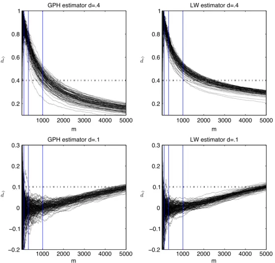
1 are fixed.

Fig. 1depicts GPH and LW estimation for the MS model. We took

µ

0

=

0

, µ

1

=

1

,

c0

=

c1

=

0

.

9, normal errors with

σ

_ϵ2

=

1

,

T

=

105and two choices of

δ

0

=

δ

1

=

0

.

8 and

δ

0

=

δ

1

=

0

.

2

cor-responding to d

=

0

.

4 and d

=

0

.

1, respectively. The top plots are the estimatesd

=



d

(

m

)

as functions of m when d

=

0

.

4, for 100 realizations. The bottom plots correspond to d

=

0

.

1. It is clearly

seen fromFig. 1that both estimators are extremely biased for a wide range of low frequencies used in estimation even for such a large sample size. For larger d

=

0

.

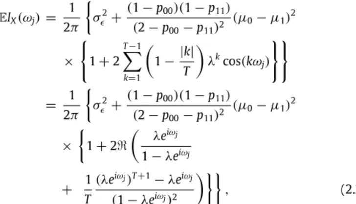
4, the estimators suggest long memory for a wide range of lower frequencies but the bias is close to zero only for a tiny subset of this range.

The difficulties with estimation can be explained further through the following argument. By using Proposition 3 inDiebold and Inoue(2001), which provides the autocovariance function of the MS model

{

XT

k

}, it can be shown that

EIX

(ω

j

) =

1 2

π



σ

2 ϵ

+

(

1

−

p00

)(

1

−

p11

)

(

2

−

p00

−

p11

)

2

(µ

0

−

µ

1

)

2

×



1

+

2 T−1



k=1



1

−

|

k

|

T



λ

k cos

(

k

ω

j

)



=

1 2

π



σ

2 ϵ

+

(

1

−

p00

)(

1

−

p11

)

(

2

−

p00

−

p11

)

2

(µ

0

−

µ

1

)

2

×



1

+

2ℜ



λ

eiωj 1

−

λ

eiωj

+

1 T

(λ

eiωj

)

T+1

₋

λ

_eiωj

(

1

−

λ

eiωj

)

2



,

(2.2)

where

ℜ

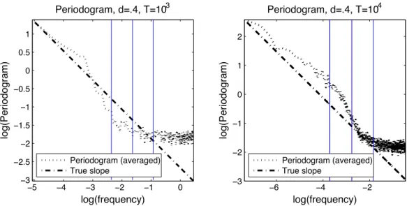
denotes the real part.Fig. 2shows the log–log plot of the expected periodogram(2.2)in plus marker, an average of 100 periodograms from simulated data in dotted line, and the slope with the long memory parameter d in dashed–dotted line, against the Fourier frequencies. Note the good agreement between the ex-pected and averaged periodograms. But also note that they deviate very significantly from the line of the expected slope determined by d.

Diebold and Inoue(2001) have also reported some numerical simulations for the MS model (see alsoYu, 2009). In figures 8 and 9, they consider the GPH estimates for the choice of m

=

T0.5, find-ing them in the interval

(

0

,

0

.

5

)

. Although these findings are con-sistent with the ones reported here (Fig. 1), we go a step further by focusing on the bias of the GPH estimator.

3. Behavior of variance of partial sum process

A disagreement of the MS model with the expected long mem-ory behavior also manifests itself in the following more basic and fundamental way. If ST

(

t

) = 

[Tt] k=1

(

X T k

−

EX T k

),

t

∈ [0

,

1], is the partial sum process of the MS model, then Proposition 3 inDiebold and Inoue(2001) can be used to show that

Var

(

ST

(

t

)) =

(

1

−

p00

)(

1

−

p11

)

(

2

−

p00

−

p11

)

2

(µ

0

−

µ

1

)

2

[

Tt

]

×



2

λ

1

−

λ

+

1

+

2

(λ

[Tt]+1

₋

_λ)

[

Tt

]

(

1

−

λ)

2



+

σ

_ϵ2

[

Tt

]

.

(3.1) This further leads to

v

T

(

t

) :=

Var



ST

(

t

)

Td+1/2



∼

Ct

,

(3.2)

as T

→ ∞

(seeBaek et al., 2014for details).

In the case of a true long memory time series, the right-hand side of(3.2)is Ct2d+1. The behavior(3.2), on the other hand, is asso-ciated with short memory and d

=

0. (As shown inBaek et al., 2014,

ST

(

t

)/

Td+1/2also converges in the sense of finite-dimensional dis-tributions to Brownian motion.)Fig. 3presents the log–log plot of

v

T

(

t

)

as a function of t, together with the expected slope equal to 1

(

d

=

0

)

. Note the good agreement between log

v

T

(

t

)

and the expected slope.

In fact, the relation(3.2)with t2d+1_{on its right-hand side gives}

Fig. 1. GPH and LW estimation for the MS model with d=0.4 and 0.1. The dashed horizontal line indicates the value of d=0.4 or 0.1. Three vertical lines correspond to m=T0.4_,T0.5_{and T}0.6_{, as rule-of-thumb choices for m.}

Fig. 2. Periodogram against Fourier frequencies in the log–log plots. The slope of the dashed–dotted line is determined by the true long memory parameter. memory parameter d, which according to(3.2)is zero for the MS

model, corresponding to short memory. From the estimation per-spective, the MS model thus behaves more like a short memory model which happens to have some long memory features as in (1.3). This claim also sheds light on the estimation result in the spectral domain: the slope of the expected periodogram inFig. 2 tends to have the zero slope at lowest frequencies (for a larger d, a much larger sample size is needed to observe the zero slope at a larger range of the lowest frequencies).

4. Conclusion

In this note, we reexamined the connection between the Markov switching model and long memory. The theoretical results ofDiebold and Inoue(2001) relate the model to long memory, but a serious bias makes the expected long memory parameter diffi-cult to observe in practice. By examining the variance of the partial sum process, we also argued that the MS model should be viewed rather as a short memory model which happens to have some long

120 C. Baek et al. / Economics Letters 124 (2014) 117–121

Fig. 3. logvT(t)against log t for the MS model with d=0.4.

Fig. 4. Log–log plots for the ON/OFF model with d=0.4 and sample sizes T=103_{and T=10}4_.

memory features. In particular, the MS model may suggest long memory through common estimators in the spectral domain.

Related to this last point, we also mention several recent works aiming at distinguishing changes-in-mean and related models from long memory. For example,Iacone (2010), McCloskey and Perron(2013) employ common estimators of long memory in the spectral domain by selecting carefully the range of frequencies to be used in estimation.Baek and Pipiras (2012, 2013)propose a method based on removing changes in mean and local Whittle es-timation.

Our findings for the MS model also stand in sharp contrast to other physical mechanisms to generate long memory. For example, the ON/OFF model (superimposed with i.i.d. noise) can be defined by(1.1)where sT

k

=

skdoes not depend on T and still takes values 0 or 1 but now sk

=



1

,

if Si

≤

k

<

Si

+

UiON

,

0

,

if Si

+

UiON

≤

k

<

Si+1

,

with Si

=

S0

+



i j=1

(

U ON j

+

U OFF

j

)

and independent collections

{

UON

j

}

and

{

UjOFF

}

of i.i.d. positive random variables. (S0is a special

random variable to ensure that skis stationary.) Such an ON/OFF model is long memory as long as the distribution F

=

FONof

{

UjON

}

or F

=

FOFFof

{

UjOFF

}

is heavy-tailed, that is, 1

−

F

(

u

) ∼

cu

−α

_,

_as

u

→ ∞, where

α ∈ (

1

,

2

)

. The long memory parameter d is related to

α

through d

=

(

2

−

α)/

2.

Fig. 4presents the log–log plots of the averaged periodogram against Fourier frequencies for the ON/OFF model where ON times are chosen to be Pareto with

α =

1

.

2 (corresponding to d

=

0

.

4),

c

=

501.2_{, and OFF times follow the exponential distribution with}

mean 150. The noise variance is

σ

2

ϵ

=

1 as in the MS model

simu-lations, and the results are based on 100 replications. As seen from the plots, the log of the periodogram exhibits a linear behavior with the slope close to the true one for a number of low frequencies con-sidered.

Acknowledgments

We would like to thank the Editor and an anonymous Referee for many useful comments and suggestions.

The research of the second author has been financed by Portuguese Public Funds through FCT (Fundação para a Ciên-cia e a Tecnologia) in the framework of the project PEst-OE/EGE/UI4105/2014. Financial support from FEDER and FCT

(research grant PTDC/EGE-ECO/122820/2010) is also gratefully ac-knowledged. The research work of the third author was supported in part by NSA Grant H98230-13-1-0220.

References

Baek, C., Fortuna, N., Pipiras, V., 2014. Convergence of the long memory Markov switching model to Brownian motion, Technical Note. Available athttp://www. stat.unc.edu/faculty/pipiras.

Baek, C., Pipiras, V.,2012. Statistical tests for a single change in mean against long-range dependence. J. Time Ser. Anal. 33 (1), 131–151.

Baek, C., Pipiras, V., 2013. On distinguishing multiple changes in mean and long-range dependence using local Whittle estimation, Preprint. Available at

http://www.stat.unc.edu/faculty/pipiras.

Beran, J., Feng, Y., Ghosh, S., Kulik, R.,2013. Long-Memory Processes Probabilistic Properties and Statistical Methods. Springer, Heidelberg.

Diebold, F.X., Inoue, A.,2001. Long memory and regime switching. J. Econometrics 105 (1), 131–159.

Geweke, J., Porter-Hudak, S.,1983. The estimation and application of long memory time series models. J. Time Ser. Anal. 4 (4), 221–238.

Granger, C.W.J.,1980. Long memory relationships and the aggregation of dynamic models. J. Econometrics 14 (2), 227–238.

Iacone, F.,2010. Local Whittle estimation of the memory parameter in presence of deterministic components. J. Time Ser. Anal. 31 (1), 37–49.

McCloskey, A., Perron, P.,2013. Memory parameter estimation in the presence of level shifts and deterministic trends. Econometric Theory 29 (06), 1196–1237.

Mikosch, T., Resnick, S., Rootzén, H., Stegeman, A., 2002. Is network traffic approximated by stable Lévy motion or fractional Brownian motion? Ann. Appl. Probab. 12 (1), 23–68.

Robinson, P.M.,1995. Gaussian semiparametric estimation of long range depen-dence. Ann. Statist. 23 (5), 1630–1661.

Robinson, P.M. (Ed.), 2003. Time Series With Long Memory. In: Advanced Texts in Econometrics, Oxford University Press, Oxford.

Smith, A.,2005. Level shifts and the illusion of long memory in economic time series. J. Bus. Econom. Statist. 23 (3), 321–335.

Willinger, W., Taqqu, M.S., Sherman, R., Wilson, D.V.,1997. Self-similarity through high-variability: statistical analysis of ethernet LAN traffic at the source level. IEEE/ACM Trans. Netw. 5 (1), 71–86.

Yu, W.-C.,2009. Markov switching and long memory: a Monte Carlo analysis. Appl. Econ. Lett. 16 (12), 1205–1210.