M
ASTER IN
F
INANCE
M
ASTER
F
INAL
W
ORK
D
ISSERTATION
T
ANGIBLE AND
I
NTANGIBLE
I
NVESTMENT OF
P
ORTUGUESE
F
IRMS IN
T
RADITIONAL
S
ECTORS
(2004-2011)
M
ASTER IN
F
INANCE
M
ASTER
F
INAL
W
ORK
D
ISSERTATION
T
ANGIBLE AND
I
NTANGIBLE
I
NVESTMENT OF
P
ORTUGUESE
F
IRMS IN
T
RADITIONAL
S
ECTORS
(2004-2011)
D
IANA
F
ILIPA
C
ARREIRA
S
OUSA
S
UPERVISION:
ACKNOWLEDGMENTS
I’m deeply grateful to Prof. Dra Elsa Maria Nobre da Silva Fontainha for helping me to construct the present investigation and by dedication and competence in research orientation. This research would not have been possible without her precious assistance.
Thanks to my parents for their effort that allowed me to finish this degree and my brother for his incentive and understanding during these months as well as my colleagues for their support.
ABSTRACT
This investigation studies the investment in tangible and intangible assets in Portuguese firms of traditional manufacturing sectors. The empirical analysis uses accounting firm-level panel data covering the period 2004-2011. Several specifications for investment behavior equations are tested and different estimation methodologies are applied (pooled OLS, FE - Fixed Effects and RE - Random Effects). Key results emerge: the recent crisis has a strong and decisive negative influence on tangible and intangible investment; sales expectations, return on assets, gross operating profits and investment/cash flow sensitivities contribute positively to total investment; capital stock and wages show weak effects on total investment; and exports, rather than the total sales, have a positive impact on intangible investment. The analysis by size categories (small, medium and large firms) and subsectors (Food Products, Textiles, Wearing, Footwear, Wood and Furniture) reveal heterogeneous dynamics and explanations for investment behavior.
Key words: tangible investment, intangible investment, business cycle, real capital, traditional sectors, Portugal
INDEX
Acronyms and Abbreviations List ... VII
Introduction ... 1
1. Literature Review ... 4
1.1. Concepts and Measurement: Tangible and Intangible Investment ... 4
1.2. Determinants of Investment Behavior ... 6
1.3. The Investment in Portuguese Firms ... 12
2. Empirical Analysis ... 14
2.1. Database: Integrated Business Accounts System (SCIE) and Sample ... 15
2.2. Investment Dynamics ... 16
2.3. Methodology: Modelling and Variables ... 17
2.3.1. Dependent and Independent Variables ... 18
2.3.2. Sets of Analysis and Model Specifications ... 20
3. Results and Discussion ... 22
4. Conclusions and Suggestions for Futures Research ... 33
References ... 37
Appendixes ... 42
Appendix A. Business Cycle, Databases and Samples ... 42
Appendix B. Description of Variables ... 48
Appendix C. Linear Models ... 49
Appendix D. Descriptive Statistics and Correlations ... 50
Appendix E. Summary Results for Investment Models ... 55
Appendix F. The Portuguese Investment Qualitative Survey ... 56
INDEX OF TABLES TABLE IEMPIRICAL STUDIES OF INVESTMENT IN PORTUGAL ... 13
TABLE IIDESCRIPTION OF DEPENDENT AND INDEPENDENT VARIABLES ... 18
TABLE IIIREGRESSION ANALYSIS OF TOTAL INVESTMENT (2004-2011) ... 23
TABLE IVREGRESSION ANALYSIS OF SPECIFIC INVESTMENT (2010-2011) ... 24
TABLE VBREUSCH-PAGAN (LM) AND HAUSMAN TEST ... 25
TABLE VITOTAL INVESTMENT BY SECTOR:MODEL 1 ... 27
TABLE VIITOTAL INVESTMENT BY SECTOR:MODEL 2 ... 27
TABLE VIIITOTAL INVESTMENT BY SIZE:MODEL 2 ... 28
INDEX OF TABLES IN APPENDIX
Appendix A. Business Cycle, Databases and Sample
TABLE AIMANUFACTURING FIRMS BY TRADITIONAL SECTOR (2004-2011) ... 42
TABLE AII TRADITIONAL SECTOR FIRMS BY SIZE CATEGORIES(2004-2011) ... 42
TABLE AIII TURNOVER AND TOTAL OF EMPLOYEES BY SIZE (2011) ... 43
TABLE AIV SHARE OF TURNOVER AND TOTAL EMPLOYEES IN % ... 43
TABLE AVINVESTMENT STRUCTURE BY FIRM (2010-2011) ... 43
TABLE AVIINVESTMENT RATEMEAN BY SECTOR (2004-2011) ... 44
TABLE AVII INVESTMENT RATE MEAN BY SIZE CATEGORIES (2004-2011) ... 44
Appendix B. Description of variables TABLE BI TANGIBLE INVESTMENT CATEGORIES ... 48
TABLE BII INTANGIBLE INVESTMENT CATEGORIES ... 48
TABLE BIII DEFINITION OF FIRM-LEVEL VARIABLES TESTED BUT NOT INCLUDED IN THE MODELS ... 48
Appendix D. Descriptive Statistics and Correlations TABLE DI SUMMARY STATISTICS FOR DEPENDENT VARIABLES ... 50
TABLE DII SUMMARY STATISTICS FOR DEPENDENT VARIABLES BY SECTOR ... 50
TABLE DIII SUMMARY STATISTICS FOR DEPENDENT VARIABLES BY SIZE ... 51
TABLE DIV SUMMARY STATISTICS FOR INDEPENDENT VARIABLES ... 51
TABLE DV SUMMARY STATISTICS FOR INDEPENDENT VARIABLES BY SECTOR ... 51
TABLE DVI SUMMARY STATISTICS FOR INDEPENDENT VARIABLES BY SIZE ... 53
TABLE DVIICORRELATION VARIABLES OF MODEL 1 AND 2 ... 54
TABLE DVIII CORRELATION VARIABLES OF MODEL 3 AND 4 ... 54
Appendix E. Summary Results for Investment Models TABLE EI MAIN QUALITATIVE RESULTS FOR TOTAL INVESTMENT MODEL BY SECTOR . 55 TABLE EII MAIN QUALITATIVE RESULTS FOR TOTAL INVESTMENT MODEL BY SIZE... 55
INDEX OF FIGURES IN APPENDIX Appendix A. Business Cycle, Databases and Sample Figure A1. Gross Fixed Capital Formation - Investment (% of GDP) ... 45
Figure A2. Investment Rate in the Portuguese Traditional Sector (2004-2011) ... 45
Figure A3. Investment Rate by Size, Portuguese Traditional Sectors (2004-2011) ... 46
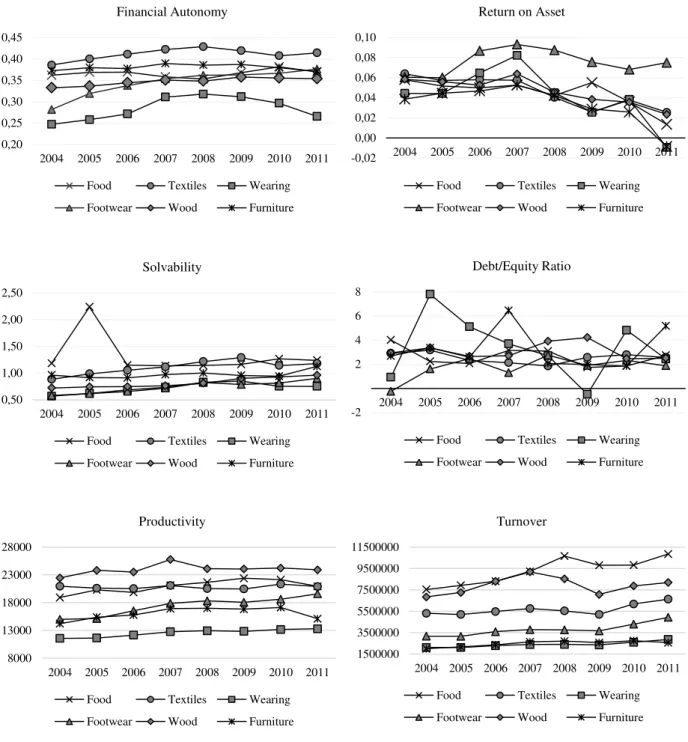
Figure A4. Financial Ratios and Variables by Sector (2004-2011) ... 47
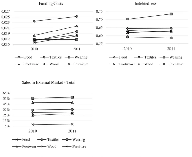
Figure A5. Financial Ratios and Variables by Sector (2010-2011) ... 48
Acronyms and Abbreviations List
AMECO Annual Macro-Economic Database [European Commission]
BdP Banco de Portugal [Bank of Portugal]
CAE-Rev.3. ClassificaçãoPortuguesa das Atividades Económicas, Revisão 3
CBSD Central Balance-Sheet Database
CF Cash Flow
EC European Commission
ECB European Central Bank
EU European Union
Eurostat Statistical Office of the European Communities FDI Foreign Direct Investment
FE Fixed Effects
GAVfc Gross Added Value at factor costs
GDP Gross Domestic Product GFCF Gross Fixed Capital Formation GMM Generalized Method of Models
GPO Gross Profit Operation [Excedente Bruto de Exploração]
IAS International Accounting Standards [Norma Internacional de Contabilidade]
ICI Inquérito Qualitativo de Conjuntura ao Investimento [Statistics Portugal]
IES Informação Empresarial Simplificada [Simplified Business Information]
IFRS International Financial Reporting Standards
IS Investment Survey [Eurostat]
NACE Nomenclature generale des Activites economiques dans les Communautes Europeennes [Eurostat]
NCRF Norma Contabilística e de Relato Financeiro
OECD Organization for Economic Co-operation and Development OLS Ordinary Least Squares
p.p percentage point
POC Plano Oficial de Contabilidade
POLS Pooled OLS
R&D Research and Development [I&D: Investigação e Desenvolvimento]
RE Random Effects
ROA Return On Assets
SAFE Survey on the Access to Finance of Enterprises
SCIE Sistema de Contas Integradas das Empresas [Integrated Business Accounts System]
SME Small and Medium Enterprises SNA System Nacional Accounts
SNC Sistema de Normalização Contabilística
UK United Kingdom
UN United Nations
US United States
VABcf Valor Acrescentado Bruto a custo de fatores
Introduction
For its pro-cyclical aggregate demand, low levels of business investment spoil the future growth of the economies in terms of production and employment (Banerjee, Kearns & Lombardi, 2015). The uncertainty from the instability of the Portuguese economy, the restrictions in financing conditions associated with the indebtedness of companies and the limitations imposed on the foreign demand determine the weak position of investment in Portugal in recent years (BdP, 2012). The real investment of Portuguese companies from 2008 to 2009 had a deep decrease: 9.2% in Gross Fixed Capital Formation (GFCF); and 3.6% in investment in non-financial firms (Eurostat, 2015c). For an understanding of the evolution of investment in recent years, it is relevant to grasp the factors that drive private investment.
This research aims to analyze the factors that explain the investment in tangible and intangible fixed assets in Portuguese companies of the traditional manufacturing sector from 2004 to 2011. It takes advantage of a very rich accounting firm-level database Sistema de Contas Integradas das Empresas (SCIE) which includes yearly, about 43,000 observations. The choice of six sectors (Food Products, Textiles Wearing, Footwear, Wood and Furniture1) is motivated by their economic relevance and performance. They correspond to a large share in the national production (INE, 2015), more than one third of the turnover in manufacture (37.98% in 2004 and 34.24% in 2011) and about half of the employment in manufacture (52.36% in 2004 and 49.87% in 2011)2. Additionally, the six sectors represent about one third of the sales in foreign market (INE, 2015) and despite being classified as “Low-technology” sectors (Eurostat,
1Nomenclature general des Activites economiques dans les Communautes Europeennes (NACE), Section C: Manufacturing (10,
13-15, 16, 31). Adapted from Classificação Portuguesa das Actividades Económicas (CAE).
2015b) they presented, in Portugal, improved recovery after the crisis shock compared to other European countries (Eurostat, 2013).
In the present dissertation, the focus is on the real investment3 and the investment in intangible assets receives particular attention in order to shed some light on the innovation in the traditional manufacturing sectors.
Existing models of investment behavior follow diverse economic schools (e.g. Keynesian or Neoclassical) that adopt different types of approach (e.g. macroeconomic or microeconomic; dynamic or static) and the empirical applications use various data sources (e.g. survey data or accounting data). In this dissertation, following the empirical work done in the field, is rooted in the mains theories about the behavior of business investment: the accelerator model; the neoclassical model; the Q-Tobin; and the Euler Equation. Two surveys of reference published in the Journal of Economic Literature are Chirinko (1993) and Jorgenson (1971).
The Keynesian accelerator model establishes a linear relation between the current net investment and the expected changes in output based on demand evolution (Barkbu, Berkmen, Lukyantsau, Saksonovs & Schoelermann, 2015; Clark, Greenspan, Goldfeld & Clark, 1979; Fazzari, Hubbard & Petersen, 1988; Jorgenson, 1971; Oliner, Rudebusch & Sichel, 1995; Von Kalckreuth, 2001)
The Neoclassical model focuses on the response of firms to change in relative prices of the productive factors based on a production function that establishes the relation between the capital stock and the output (Barkbu et al., 2015; Bond & Van Reenen, 2007; Chirinko, 1993; Clark et al., 1979; Fazzari et al., 1988; Jorgenson, 1967; Jorgenson & Handel, 1971; Oliner et al., 1995).
3 Given the study focus and the data availability, two specific steam of the investment literature: the investment on financial assets
The Q-Tobin theory (Barkbu et al., 2015; Bond & Van Reenen, 2007; Chirinko, 1993; Clark et al., 1979; Fazzari et al., 1988; Oliner et al., 1995) and the Euler Equation
(Barkbu et al., 2015; Bond & Van Reenen, 2007; Bond, Elston, Mairesse & Mulkay, 2003; Chirinko, 1993; Clark et al., 1979; Janz, 1997; Oliner et al., 1995) relate to the volatility and the instability that the investment has over time in financial markets. These two theories are not subject to specific empirical analysis in this dissertation because the main database used (SCIE) does not include any information on the cost of capital and the value of the company in the financial market.
The previous studies about the explanatory factors for real investment in Portugal indicate that they are: the size of the company; the growth of sales company; the macroeconomic context; the share of sales in the external market; and the financial situation of the company (Barbosa, Lacerda & Ribeiro, 2007; Barkbu et al., 2015; Farinha & Prego, 2013; Pina & Abreu, 2012).
This dissertation, using panel data analysis, tests several financial and economic variables to explain global business real investment and also by categories of investment (tangible and intangible), by sectors of activity and by firm size4. The Return On Assets (ROA), the Cash Flow (CF), the stock of capital, sales expectations, sales in the external markets, Research & Development (R&D) intensity and the crisis are some of the successfully tested explanatory variables.
theoretical approaches; (ii) studying independently the investment in intangible assets filling one gap identified in the literature about intangibles (Haskel, Jona-Lasinio & Iommi, 2012; Marrocu, Paci & Pontis, 2012); (iii) analyzing the impact on firm investment caused by the economic and financial crisis and the sovereign debt; and (iv) investigating in detail the differences among the investment behavior by sector and firm size categories .
This dissertation is organized into four sections. In section 1, it is carried out the literature review, which is divided in three subsections: conceptual aspects; explanatory theories of investment; and a survey of previous studies for Portugal. The section 2
presents the database, the sample, and the methodologies adopted. Section 3 shows and discusses the results. Finally, in section 4 the conclusions and suggestions for future researches are listed.
1. Literature Review
1.1. Concepts and Measurement: Tangible and Intangible Investment
The investment discussed in this research is the real investment that involves some sort of asset, is related to the company's activity and is creator of productive capacity. The real investment includes tangible and intangible assets, that can be used
The International Financial Reporting Standards (IFRS, 2015, p. 1), define
tangible assets (property, plant and equipment) as “tangible items that are held for use in the production or supply of goods or services, for rental to others, or for administrative purposes (Table BI); and are expected to be used during more than one
period”5
. Tangible assets are also defined as assets with physical investment of company property (Haskel et al., 2012, p. 2) and investment in nonresidential structures (Oliner et al., 1995, p. 807).
There is a strong debate on the definition and categories of intangible assets. In contrast to tangible assets, for the intangible assets it is difficult to establish a relationship between the quantity of tangible and physical investment (Young, 1998).
Intangible assets are “an identifiable non-monetary asset without physical substance” (IFRS, 2015) (Table BII). Different categories and typologies are proposed to define this type of investment. Following Young (1998), the intangible investment includes six categories: computer-linked (e.g. software); technology and production (e.g. R&D); human sources (e.g. learning by doing and in activities to improve health and motivation of the employees); organization of the firm; marketing and sales; and industry-specific (e.g. mineral exploration). Recently, Haskel et al. (2012) adopts another typology considering that the intangible investment includes: computerized information (e.g. software); innovation property (e.g. mineral exploration and R&D); and economic competencies (e.g. advertising).
The analysis of intangible investment behavior has an increasing role for understanding the total of investment (Marrocu et al., 2012). Corrado, Hulten and Sichel (2005) concluded that, recently, in United Kingdom (UK) and United States (US), the
investment in intangible assets overtakes the investment in tangible assets. Nevertheless, although theoretically relevant to business growth, Gross Domestic Product (GDP) and employment, the empirical analysis about intangible assets is still insufficient (Corrado et al., 2005 and 2009; EC, 2011; Haskel, et al., 2012; Marrocu et al., 2012). Timmer
(EC, 2011) states that “if we want to understand the effects of intangibles on economic
growth, perhaps a new approach is needed to replace the traditional growth accounting”
(p. 17) and Corrado (EC, 2011) agrees with him claiming that “there is ‘a big hole’ with
respect to intangibles accounting” (p. 25).
There are different lines to study the intangible assets: (i) the inclusion in the accounting (national and firm level) and in firms’ behavior (e.g. EC, 2011 and Bond & Van Reenen, 2007), as it is done in the present research; (ii) the effect of intangible on economic growth (Corrado et al., 2009; Solow, 1957); (iii) the impact on productivity (Bontempi & Mairesse, 2015; Marrocu et al., 2012; Haskel et al., 2012); and (iv) the effect on competition (Cañibano, Garcia-Ayuso & Sánchez, 2000).
1.2. Determinants of Investment Behavior
Accelerator Models – simple and flexible
The accelerator theories are related to the demand, to the optimal stock of capital and to the cost of capital (Barkbu et al., 2015; Clark et al., 1979; Fazzari et al., 1988; Jorgenson, 1971; Oliner et al., 1995; Von Kalckreuth, 2001). The accelerator
models assume a relationship between the net investment and the expected change in the
output or sales that are made through an adjustment process of the net investment and how the expectations about the output are formed (Clark et al., 1979). Variations in the desired output will involve variations in desired stock of capital and, consequently, changes in the net investment (i.e. investment excluding the replacement of capital). Investment depends on the adjustment process of the capital stock to the desired capital stock and, in this model, it can be assumed that the desired stock of capital is proportional to the output (Clark et al., 1979; Oliner et al., 1995).
In the flexible accelerator model, the investment in each period contributes partially to attain the desired stock of capital. The aggregate investment is explained using a “distributed lag function, relating the actual level of capital to past desired levels of capital” (Jorgenson, 1971, p. 1111). In this model, the output, the internal funds, and the costs of external funds have also effect on investment (Jorgenson, 1971).
Neoclassic theory of optimal capital accumulation
The neoclassical model is related to output dynamics and is based on production function, costs and prices (Barkbu et al., 2015; Bond & Van Reenen 2007; Chirinko, 1993; Clark et al., 1979; Fazzari et al., 1988; Jorgenson, 1967; Jorgenson & Handel, 1971; Oliner et al., 1995). The neoclassic theory of optimal capital accumulation, ‘the typical model to explain the investment’ (Jorgenson, 1967), has several versions.
project/firm by maximizing profits and, according Bond and Van Reenven (2007, p. 6)
the firm’s goal is to “maximize the value of the equity owned by its shareholders”. The
level of investment depends on the relation between capital and output, relation which is done by a production function, which allows to determine the optimum value for the rental cost of capital (Jorgenson, 1971). A higher real cost of capital implies a lower level of desired capital stock and, consequently, a lower level of desired investment (Barkbu et al., 2015). In this model, the desired change in capital is related to the function of the real cost of capital assumed to be equal to the marginal productivity (Jorgenson, 1971; Oliner et al., 1995). The approach to investment done by a production
function relates the marginal productivity of factors to the factor’s earnings. For example, if a Cobb-Douglas function is adopted, assuming implicitly perfect competition, in the optimum, the wages are equal to the marginal productivity of labor and the rental cost of capital must be equal to the marginal productivity of capital stock. If the relative price of the factors (capital and labor) changes, it is expected that the relative intensity of use of each factor also change. Bond & Van Reenen (2007) studying in separate the investment and the employment incorporates the average wage, computed by the ratio between the wage bill of each firm and the number of workers in the firm. To Chirinko (1993, p. 1876) “prices (taxes, interest rates), quantities (output and liquidity) and autonomous shocks (“animal spirits” and technology)” are determinants of investment. This theory was empirical tested for the manufacture and in aggregate level by Jorgenson and Handel (1971).
(1) where is the capital stock at t-1; Δ is the firm’s variation of the desired capital stock; and is the depreciation rate of the stock of capital.
Q-TobinTheory and Euler Equation
Substantial part of the investment literature uses financial market data (Bond & Van Reenen, 2007) to study the volatility, the non-symmetric, and the instability of investment. Two theories used almost exclusively financial data: the Q-Tobin (Barkbu et al., 2015; Bond & Van Reenen, 2007; Chirinko, 1993; Clark et al., 1979; Fazzari et al., 1988; Oliner et al., 1995) and the Euler Equation (Barkbu et al., 2015; Bond & Van Reenen, 2007; Bond et al., 2003; Chirinko, 1993; Clark et al., 1979; Janz, 1997; Oliner et al., 1995).
The Q-Tobin theory establishes a link between the investment rate and the Q
variable that is “the ratio of the discounted future revenues from an additional unit of capital to its purchase price” (Chirinko, 1993, p. 1988). This model allows to measure, at market prices the investment opportunities (Fazzari et al., 1988) and uses the real cost of capital to measure the investment (Bond & Van Reenen, 2007). However, Q-Tobin theory is considered by some authors as an insufficient model to explain reality due to inconclusive empirical results (for example, “the statistical significance of [the
Q-Tobin ratio] and the fit of the equation” (Chirinko, 1993, p. 1891) are weak and also
because there are “data measurement issues at aggregate level” (Barkbu et al., 2015, p. 14)).
1997). The adjustment of real investment to desired investment follows a model with lags. For example, the Euler equation model proposed by Bond et al. (2003, p.156) is:
(2) s.t .
where is the expectation operator conditional to information available in period t; is the nominal discount factor between period t and t+j;
where is variable factor input; is the price of the output; the production function gross of adjustment cost; the adjustment cost function and the depreciation rate. The opinions regarding this theory are controversial. Bond et al. (2003) consider it a useful model because it captures the influence of expectations on the profitability of the investment and controls the influence of financial variables on the expectations on future profitability. On the contrary, other authors consider the Euler Equation unsuitable (Chirinko, 1993; Oliner et al., 1995). Chirinko (1993) states that the Euler equation “is based on a limited amount of information from the firm's optimization problem. This limitation may prove beneficial if the information contained in the other equations is suspect or more
sensitive to certain types of misspecification.” (p.1894). Oliner et al. (1995) also argue
against the Euler equations because they “produce extremely poor forecasts of
investment for both equipment and nonresidential structures” (p. 807).
Expectations and uncertainty
the creation of future expectations about output and sales (Chirinko, 1993) and expectations about future rentability are based on past and current CF (Clark et al., 1979).
The uncertainty about the profitability and economic conditions affects the returns, the rentability, the funding resources and the funding cost expectations (Banerjee et al., 2015). These authors, covering the period of 1990-2014 for Germany, Canada, Japan, Italy, UK and US, conclude that the main reasons for investment to be weak is the uncertainty in relation the future economic situations of the each country, the profitability of the investment opportunities and the return to the application of new capital. The level of uncertainty perceived by the investor differs across investors because it depends on several factors (e.g. type of project, technology and firm’s market power). The risk perception can be incorporated into investment decisions by several forms (e.g. though the required rate of return) (Farla, 2013; Pindyck, 1990). Probably, expectations and uncertainty are the main reasons why it is so difficult to find suitable models to explain the investment behavior.
Tight monetary policies, imposing difficult access and reducing granting of bank loans are also factors that may restrict the investment (Kothari, Lewellen & Warner, 2014) since it makes more expensive the investment by using external funds (Fazzari et al., 1988). The empirical results about this issue are mixed. For example, Von Kalckreuth (2001) demonstrates that even companies without financial constraints do not invest if there are in risky situations.
The investment is also analyzed by business surveys (e.g. Inquérito Qualitativo
de Conjuntura ao Investimento (ICI) is the business investment survey (INE, 2014a) in
information from the business responsible the expectations of entrepreneurs about future sales, the objectives and main obstacles to investment (Farla, 2013; Jorgenson & Handel, 1971; Maria & Serra, 2008).
Summarizing, there are diverse theories that try to explain investment behavior and consequently, the empirical approaches are also diverse concerning model specifications, databases and methodologies. The empirical studies are being improved as more detailed and representative databases become available from administrative, accounting, and survey sources. However, the difficulties to explain and to forecast private investment remain. The statement of Caballero, Engel, Haltiwanger, Woodford and Hall (1995) about the obstacles faced by investors is still valid and also explain the difficulties of the researchers about investment behavior: “there are serious theoretical obstacles, stemming mostly from the richness of the cross-sectional and time-series scenarios faced by actual investors, from the complexity of the investment technologies available to them, and from the myriad incentive problems that these economic agents face. There are at least as complex, and perhaps in-surmountable, data problems” (p. 1).
1.3. The Investment in Portuguese Firms
This section presents and discusses the empirical literature about the investment in Portugal mainly using a microeconomic approach and two macroeconomic approaches analyzed Portugal among European context (Table I summarizes). The financial aspects that include the recent period of crisis are highlighted.
conditioned the investment of European companies in the period 1998Q2-2012Q1; in Portugal, the corporate leverage and the financial constraints had negatively affected private investment. In line with these results, Farinha and Prego (2013) concluded that the Portuguese investment between 2006 and 2011 is negatively associated with the cost of capital, the interest debt burden and the indebtedness increase.
TABLE I
EMPIRICAL STUDIES OF INVESTMENT IN PORTUGAL
Authors (Year)
Database(s)
Period of information (Frequency)
Countries
(Unit of analysis) Main conclusions
Barbosa et al. (2007)
Central Balance-Sheet Database (CBSD) of
Banco de Portugal
based on Simplified Business Information (IES)
1995-2006 (Annual)
Portugal
(Portuguese non-financial
corporations)
The financial situation of firms is essential to the evolution of investment (interest, indebtedness and size have a negative impact on investment as opposed to sales and profitability).
Mixed results of sensibility of export companies.
Barkbu et al. (2015)
AMECO, WEO,
EUROSTAT, ECB 1990-2012/13 (Quarterly)
Portugal,
Germany, France,
Italy, Spain,
Ireland and
Greece (countries)
The corporate leverage and
financial constraints have a
negative impact on investment.
Farinha & Prego (2013)
CBSD of Banco de Portugal (based on IES)
2006-2011 (Annual)
Portugal
(Portuguese non-financial
corporations of
private sector)
The financial situation of firms is essential to the evolution of investment (interest, funding costs and indebtedness have a negative impact on investment as opposed to sales and profitability).
Results heterogeneous by size.
Pina & Abreu (2012)
EUROSTAT, OECD, BdP
2000-2010
Portugal and Euro Area countries (countries)
Between 2005-2011 there was a significant drop in total exports.
Source:Author’s construction based on Barbosa et al. (2007); Barkbu et al. (2015); Farinha & Prego (2013); Maria & Serra (2008) and Pina & Abreu (2012).
lack of investment opportunities. Similar results are obtained for Portugal over the period 2008-2014, according to the ICI6.
The relationship between investment/CF sensitivity and financial constraints is studied by several authors and suggest some debate since get to opposite results. For example, Mizen and Vermeulen (2005), analyzing UK and Germany, affirmed that the private investment is more sensitive to the CFs fluctuations for companies financially constrained. Also for Portugal in 1995-2005, Barbosa et al. (2007) and Farinha and Prego (2013) conclude that investment is less sensitive to financial pressure for large companies.
In brief, the empirical literature for Portugal indicates that the main determinants of investment in Portugal are: the size of company, the sales growth, the macroeconomic context, the share of exports on sales and the financial position of the company (see fourth column in Table I).
2. Empirical Analysis
After the presentation of theories and results about investment behavior (points 1.2 and 1.3) it is evident that there are of difficulties to parametrize the investment behavior. Additionally, to have a full image of investment behavior a large scope of
information is needed (e.g. institutional data; firm’s governance and strategies detailed;
detailed accounting data). The empirical analysis carried out in the present research takes advantage of a very rich Portuguese accounting database (SCIE), much richer than other studies in the literature (e.g.: panel data for eight years; distinction between investment in tangible and intangible assets) but it does not include information about the strategy and the governance in each firm.
2.1. Database: Integrated Business Accounts System (SCIE) and Sample
This research has as main informative support the accounting microdata of SCIE for the period 2004-2011. SCIE is an annual database based on administrative data following IES (INE, 2014b, 2015) and accessible to the scientific community through protocol. This database covers an extensive list of accounting variables (about 80 for the period 2004-2009 and 262 for 2010-2011) allowing the building of financial ratios.
The empirical studies about investment behavior are based on diverse units of analysis (firm, sector, or countries) and databases (e.g. Amadeus, AMECO, CBSD, US Industrial Census and Compustat and Qualitative Surveys). The adoption of SCIE as the main database, has clear advantages over other databases like Amadeus database (BVD, 2015) which is used for example in Marrocu et al. (2012) and Mizen and Vermeulen (2005) because SCIE covers better the universe of the Portuguese firms. SCIE provides detailed information by sector (5 CAE code digits desegregation), rather than AMECO database (Santos, 2007) used by Banerjee et al. (2015) and Barkbu et al. (2015). The type of data included in SCIE is similar to CBSD (BdP, 2015b) used by Barbosa et al. (2007) and Farinha and Prego (2013). Using SCIE database it is possible to analyze a balanced panel data like other studies have done (Barbosa et al., 2007; Bond & Van Reenen, 2007; Bond et al., 2003; Caballero et al., 1995; Farinha & Prego, 2013; Janz, 1997; Marrocu et al., 2012). On contrary, business survey data used by several authors (Farla, 2013; Jorgenson & Handel, 1971; Maria & Serra, 2008) do not allow to build balanced panel data.
for micro, small, medium and large companies was characterized in detail7 (Table AI). The balanced panel specially built for the current research includes 1,273 firms observed in eight consecutive years which corresponds to 10,184 observations of small, medium and large firms. Because the composition of the database (number of variables) is not constant across time specific samples were built by periods and investment types (e.g. tangible and intangible assets).
2.2. Investment Dynamics
The analysis of the investment evolution in these sectors is measured by the
investment rate by firm following calculation formula defined by INE (2014b, 2015) and Eurostat (2015a): GFCF divided by Gross Added Value at factor costs (GAVfc).
Figures A1 and A2 in Appendix A illustrate the difference between the behavior of Portuguese investment comparing with Euro Area investment (Figure A1), and the investment in the traditional sectors (Figure A2). The mean of investment rate in traditional sector during the period 2004-2011 has lower values, compared to Portuguese investment, respectively 13.6% and 20.3%. The profile across time is also distinct in both groups: for the global values the maximum value is attained in 2008 and in traditional sectors the maximum values are attained in year 2006 and 2008. The crisis, evidenced in the decline 2008-2009 for the whole private sector (Figure A1), had a larger impact compared to the rate of investment in the traditional sector. The tangible-intangible mix of the investment by firms are heterogeneous by sector and by size. The main component of investment is the tangible investment which represents about 97% of the investment by sector (Table AV). Textiles has the highest relative share of investment in intangibles in 2010 (3.80%) and the second highest share in 2011
(4.63%) and, by contrast, Footwear has the lowest share in 2010 (1.64%) and 2011 (1.03%). In 2010-2011, all of sectors reduced tangible investment by firm (Table AV) with two exceptions: Footwear which increased and Food Products that remained constant. In tangible investment, the Food Products has the highest intensity and Wearing has the lowest share in 2010-2011. In intangible investment, the levels of investment are higher in the Footwear at the beginning of the period (2004) but in middle period, the Food Products (2006-2007) and Furniture (2008-2009) present the best share (Table AVI). The Footwear and the Wood show a good financial performance measure by ROA and the Wood and Textiles have the higher productivity (Figure A4).
The large firms, compared to medium and small firms, have a larger fluctuation of investment and more concentrated in time, and higher shares in total investment in 2006 and 2008. However, from 2010 on, the small companies present the highest share of investment (Figure A3). The large firms show the highest rate in intangible investment, despite of share have been decreasing during last observed years (9.31% in 2006 and 0.94% in 2011) (Table AVII).
2.3. Methodology: Modelling and Variables
into account individual heterogeneity (unobservable fixed effects specific of firms) (Arellano & Bond 1991; Bond, 2002; Cameron & Trivedi, 2010; Wooldridge, 2010). The software used in all estimations is STATA 12®.
There are different linear panel-data models (Cameron & Trivedi, 2010). In this research the models adopted are: Pooled OLS (POLS), Fixed Effects (FE) and Random Effects (RE). The use of this empirical strategy follows Aivazian, Ge & Qiu (2005). The empirical strategy starts with the estimation of POLS where the observations are pooled across time and cross-sectional unit. After, FE are tested where the unobserved effects are correlated with the explanatory variables and finally RE are applied where does not exist correlation with the explanatory variables (Cameron & Trivedi, 2010; Wooldridge, 2012).
2.3.1. Dependent and Independent Variables
Based on the literature, alternative dependent variables of Investment Rate are computed and different explanatory variables are selected for the modelling of firm’s investment behavior (Table II summarizes).
TABLE II
DESCRIPTION OF DEPENDENT AND INDEPENDENT VARIABLES
Description Observ.
Dependent Variable
(including in the models 1, 2, 3 and 4)
Investment Rate
Total annual expenditure for tangible and intangible investment in relation capital stock (in percent)
(i) (ii)
Investment Tangible Rate
Total annual expenditure for tangible investment in relation the gross added value at factor costs (in percent)
-
Investment Intangible Rate
Total annual expenditure for intangible investment in relation the gross added value at factor costs (in percent)
Explanatory Variables
(including in models 1, 2, 3 and 4)
Crisis =1 if the year is between 2009 and 2011; 0 otherwise
(2004-2008) (a) (b)
Capital Stock (in 106 euros) -
ROA
Return on assets: operating income divided by total assets.
It is comparable to the firm’s unlevered return on equity. (b) (c)
(d)
Sales
Firms sales (in 106 euros) (e) (f)
(b)
Gross Operating Profit Funds raised by the company (in 106 euros) (a)
Investment/Cash Flow
sensitivity (g) (h)
(i)
Average Wage )
Average wage by employee (euros)
-
Exports )
=1 if at least 25% of sales are done in external markets; 0 otherwise
-
Funding Costs (b) (c)
R&D Personal
Number of the R&D employees in relation to the total of
employees -
Employees Number of the total employees in firm (j)
Sector
10 = 1 if sector is food products; 0 otherwise; 13 = 1 if
sector is textiles; 0 otherwise; 14 = 1 if sector is wearing; 0
otherwise; 15 = 1 if sector is footwear; 0 otherwise; 16 = 1
if sector is wood and cork; 0 otherwise; 31 = 1 if sector is furniture; 0 otherwise.
-
Size
Small companies (Size S) = 1 if the companies has between
10-45 employees; 0 otherwise; Medium companies (Size
M) = 1 if the companies has between 45-249 employees; 0
otherwise; Large companies (Size L) = 1 if the companies
has higher than 250 employees; 0 otherwise
-
Adapted from (i) Barbosa et al. (2007) (ii) Fazzari et al. (1988) (a) Kothari et al. (2014) (b) Farinha & Prego (2013) (c) Barbosa et al. (2007) (d) Neves (2012) (e) Von Kalckreuth (2001) (f) Aivazian et al. (2005) (g) Chirinko & Von Kalckreuth (2002) (h) Fazzari et al. (1988) (i) Cleary (1999) (j) Marrocu et al. (2012).
Source:Author’s construction.
investment); the financing constrains9(financial autonomy, interest, indebtedness, solvability); the share of sales in the external market (exports); the cost with employees and innovation (average wage, R&D Personal) and the cost of non-equity funding (funding costs)10.
2.3.2. Sets of Analysis and Model Specifications
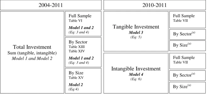
Different sets of analysis are created following the criteria: availability of data across years, type of investment (in tangible or intangible assets), sector (6 sectors) and size (3 categories). The four model specifications analyzed in detail result from a selection based on a large scope of empirical tests for each sample considered. The relation between the four models, associated samples, and tables with results are summarized in Figure 1. The models are: two for total investment using the full sample, by the six sub-sectors and by size (Model 1 and Model 2); and two when investment behavior is analyzed in separate for tangible and intangible assets (Model 3 and Model 4
respectively). Because there is an additional availability of some variables11, for the two last years of the database (2010 and 2011), two periods are considered: 2004-2011 and 2010-201112.
9 See in Appendix A.3. Figure A4 and A5 the financial ratios and variables by size over period 2004-2011 and 2010-2011. 10 See in Appendix B in Table BIII some variables tested but not include in models due to weak results.
11 For period 2010-2011 the data include, additionally to 2004-2009: Exports (expr), R&D Personal (empr&d), Interest and Funding cost (fcost); and investment tangible (invtangrate) and intangible (invintangrate) rate can be studied in separated.
12 For theoretical reasons were made apart estimates for the period 2004-2008 and 2009-2011 to test structural changes before and
Figure 1. Resume of the Models for Total, Tangible and Intangible Investment
The Total Investment is computed GFCF divided by Capital Stock (Kt); the Tangible Investment (rate) is computed tangible investment divided by GAVfc and the Intangible Investment (rate) is computed intangible investment divided by GAVfc.
(a)The model presents statistically insignificant coefficients.
Source:Author’s construction
The equation of the Model 1 is:
(3)
where investment rate ( ) is defined as the investment (GFCF) divided by capital stock is the dependent variable; is an year dummy variable; - a proxy of stock of capital of firm at time t-1; is the logarithm of return on asset;
- is the lagged value of sales of firm i. Term is the fixed effect, containing all
factors that do not vary over time; and is the error term.
Model 2 is represented by the following equation:
(4)
where the common variables with Model 1 have the same meaning previously announced and is the logarithm of Gross Operating Profit (GPO) by firms; is a proxy of investment/cash flow sensitivity of firm at time t and is the logarithm of the average wage of each firm.
2004-2011
Total Investment
Sum (tangible, intangible)
Model 1 and Model 2
Full Sample Table VI
Model 1 and 2 (Eq: 3 and 4)
By Size Table XV
Model 2 (Eq:4) By Sector Table XIII Table XIV
Model 1 and 2 (Eq: 3 and 4)
2010-2011
Tangible Investment
Model 3
(Eq: 5) By Sector
(a)
By Size(a)
Full Sample Table VII
Intangible Investment
Model 4
(Eq: 6) By Sector
(a)
By Size(a)
For tangible (Model 3) and intangible assets (Model 4) investment, the dependent variable (rate of investment) follows the definition proposed by INE (2014b, 2015). Model 3 is represented by:
(5) where dependent variable is defined as tangible investment divided by GAVfc; is dummy variable (equal to 1 if at least 25% of the sales are done in
foreign markets and equal to 0 otherwise); is the logarithm of funding cost; is the share of employees in R&D in total firm’s employment; is the logarithm of number of employees in firm; term is the fixed effect, containing all factors that do not vary over time; and is the error term.
For the Model 4, the dependent variables are equal to Model 3, but the dependent variable is defined as the intangible investment divided by GAVfc.
(6)
3. Results and Discussion
Results
Three different methodologies (POLS, FE and RE) are used to estimate the four models adopted: Model 1 and 2 (Total Investment), Model 3 (Tangible Investment) and
TABLE III
REGRESSION ANALYSIS OF TOTAL INVESTMENT (2004-2011)
Model 1 Model 2
Pooling
regression Fixed effect
Random effect
Pooling
regression Fixed effect
Random effect
Crisis -21.7022***
(-46.4497) -21.4617*** (-40.2779) -21.6861*** (-44.5189) -19.4908*** (-41.8046) -17.5443*** (-28.9722) -19.4810*** (-41.4658) Capital
Stock -0.0000*** (-6.2703) -0.0000*** (-3.4699) -0.0000*** (-4.0848) -0.0000*** (-6.4650) -0.0000*** (-3.6974) -0.0000*** (-4.1571)
1.3715*** (5.4713)
0.2436 (0.6758)
1.2794***
(4.9190) - - -
Total of
sales 0.0000*** (3.0289) (-1.3521) -0.0000 0.0000*** (2.7913) 0.0000*** (4.1029) (-0.8953) -0.0000 0.0000*** (3.0250)
- - - 0.6005*** (3.1378) (-1.1678) -0.5440 0.6084*** (3.0484)
Invest/CF
sensitivity - - - 1.4583***
(9.2438) 1.1513*** (7.3314) 1.4440*** (8.8325) Average
wage - - - -8.0343*** (-8.8284) -24.6456*** (-7.8007) -8.1749*** (-8.7576)
Intercept 41.5243*** (49.3233) 39.0274*** (33.7579) 41.2406*** (46.2289) 102.4977*** (13.4685) 272.3349*** (9.2662) 103.7354*** (13.3926)
F(X,Y) 616.84
X=4 Y=7514
504.69
X=4 Y=1267 -
492.27 X=6 Y=8299
420.93
X=6 Y=1271 -
Wald - - 2226.29 Z=4 - - 2699.08 Z=6
Prob F 0.0000 0.0000 0.0000 0.0000 0.0000 0.0000
Root MSE 21.372 - - 20.875 - -
Observation s
Groups
7,519 7,519
1,268
7,519 1,268
8,306 8,306
1,272
8,306 1,272
R-squared 0.2179 0.2468(a) 0.2525 0.2800(a)
Robust t-statistics in parentheses for POLS and FE and z-statistics for RE. Significance levels: *** 1% ** 5% * 10%. (a)Within R2.
The impacts of the variables on investment in POLS and RE had the expected signs (Table III, Models 1 and Model 2). The crisis, the stock capital (lagged) and the average wage have a negative impact on total investment. Symmetrically, the ROA, the total of sales (lagged), the GPO and investment/cash flow sensitivity have a positive impact13.
The Model 3, for tangible investment, the qualitative and statistical significance of results is weak since only two variables present statistically significant results and
one of them presents a signal that is not expected. Moreover, the model has a very low R2 in POLS (Table IV). The Model 4 for intangible investment, in POLS and RE, have the expected signal for the coefficients are the expected: exports and total of employees are positive.
TABLE IV
REGRESSION ANALYSIS OF SPECIFIC INVESTMENT (2010-2011)
Dependent variable:
Model 3 Model 4 (Full Sample) Pooling
regression Fixed effect
Random effect Pooling regression Fixed effect Random effect
Exports -1.9825*
(-1.7121) 9.7230** (2.4036) -1.9825* (-1.8176) 0.2867*** (3.0987) -0.0973 (-0.3758) 0.2493*** (2.6085) Funding
costs 1.5853*** (3.2186) 4.9504*** (3.1092) 1.5853*** (3.2667) 0.0497*** (3.2990) (-0.0685) -0.0024 0.0453*** (2.8582)
R&D
Personal (0.1024) 2.0430 -134.4824 (-1.3857) (0.0951) 2.0430 (1.5335) 7.4016 4.2866** (2.2201) (1.2431) 7.1331
Total of employees -0.8417 (-0.8897) -26.9921 (-0.9676) -4.2259*** (-3.3322) 0.1248**
(2.4336) (1.2517) 0.5649
0.1345** (2.1638)
Intercept 19.9708*** (3.3588) 130.4464 (1.2112) 19.9708*** (3.4160) (0.2319) 0.0395 (-1.0170) -1.6953 (-0.0289) -0.0058
F(4,X) X=21383.26 X=11204.73 - X=21388.11 X=1120 1.26
-Wald - - 13.71 - - 21.12
Prob F 0.0113 0.0009 0.0083 0.0000 0.2836 0.0003
Root MSE 33.888 - - 1.7109 - -
Observat. Groups
2,143 2,143
1,121
2,143 1,121
2,143 2,143
1,121
2,143 1,121
R-squared 0.0059 0.0241(a) 0.0217 0.0017(a)
Robust t-statistics in parentheses for POLS and FE and z-statistics for RE. Significance levels: *** 1% ** 5% * 10%. (a)Within R2.
The Hausman specific test compare the random effects model (null hypothesis) versus fixed effects model. The null hypothesis is rejected at the 1% at the significant level for both models, it means that the FE models is appropriate for Model 1 and Model 2. For
Model 3 and Model 4, RE is preferred.
TABLE V
BREUSCH-PAGAN (LM) AND HAUSMAN TEST Model 1
Total Investment
Model 2 Total Investment
Model 3 Tangible Investment
Model 4 Intangible Investment
LM test Chi-Sq(1)=10.00(P=0.0000) *** Chi-Sq(1)=0.81 (P=0.1844) Chi-Sq(1)=0.00 (P=0.100) Chi-Sq(1)=267.88(P=0.0000) ***
Hausman test
Chi-Sq(2)=34.82*** (P=0.0000)
Chi-Sq(4)=143.11*** (P=0.0000)
Chi-Sq(4)=9.41* (P=0.0517)
Chi-Sq(4)=4.11 (P=0.3914) Robust t-statistics in parentheses. Significance levels: *** 1% ** 5% * 10%.
The obtained results are influenced by the estimation models adopted. Through the tests carried out, the adequate models are: for Model 1 - FE and RE; for Model 2 - POLS and FE; for Model 3 - POLS and RE; and for Model 4 - RE.
Besides the Langragian Muliplier (LM) of Breusch-Pagan and the Hausman tests, to check the results’ quality, it is necessary to study if models have multicollinearity and heteroskedasticity. The multicollinearity is the correlation among independent variables and if its presence affects the efficiency of the estimated coefficients leading to incorrect conclusions (Wooldridge, 2012). Since the correlation between most of the variables (Table DVII and DVIII) is lower than 0.30, it means that collinearity is not a relevant problem in the models tested. The variance inflation factor calculation that finds out if the variance is inflated when a regressor is not orthogonal to the other regressors (Cameron & Trivedi, 2010; Wooldridge, 2012) produces the same conclusion. Consequently, the multicollinearity is not considered to be a serious problem in these models.
variables (Wooldridge, 2012). Through the Wald test and the heteroskedasticity test (Cameron & Trivedi, 2005), it is confirmed that the variance of the error term, given the explanatory variables, is not constant in all of models once the probability is zero and consequently the null hypothesis is rejected: absence of heteroskedasticity at the 1% significant level. To surpass this problem, it is used the White’s robust standard errors test (Cameron & Trivedi, 2010; Aivazian et al., 2005) which will allows getting consistent standard errors calculations. All t-statistics and z-statistics presented in Tables III and IV are taking in consideration the consistent standard errors.
The same specifications adopted to the global sample are also tested by sector of activity (6 sectors) and by firm size (3 categories) in order to verify if the variables that explain the investment for those particular sub-sectors are similar to the variables explaining the investment at more aggregate level. An initial analysis focuses on the signals of the variables (Table EI and EII) and next on its significance using the POLS. Only models that have passed into the POLS procedures were taken into account for the analysis of the FE and RE. This criterion has done due to simplicity and direct analysis of the model.
For Total Investment by sector (i.e. without distinction between tangible and intangible), the two models (Model 1 and Model 2) provide strong results only for some sectors (Food Products, Textiles, Wearing and Furniture). Table VI shows the results by sector over the period 2004-2011 for Model 1 and Table VII for Model 2.
The Model 2 is the best model for small and medium companies (see Table VIII)
expected. Applying the statistical tests previously presented, it is possible to state that the POLS is suitable though LM statistic test because the null hypothesis is not rejected at the 1% at the significant level for these subsectors and size and through Hausman test the null hypothesis is rejected at the 1% at the significant level.
TABLE VI
TOTAL INVESTMENT BY SECTOR:MODEL 1 Dependent variable:
Textiles Wearing
Pooling
regression Fixed effect
Random effect
Pooling
regression Fixed effect
Random effect
Crisis -17.8252***
(-12.8037) -16.4874*** (-10.8230) -17.7594*** (-12.6016) -26.7674*** (-22.1731) -26.5889*** (-17.0993) -26.7674*** (-21.8756)
Capital Stock -0.0000**
(-2.4217) -0.0000*** (-2.7523) -0.0000** (-2.2419) -0.0000*** (-4.4450) -0.0000** (-2.4298) -0.0000*** (-3.6378) 1.2594* (1.6651) 0.3374 (0.3752) 1.2032* (1.8484) 2.2812*** (3.6970) 0.7424 (0.8319) 2.2812*** (3.6767)
Total of sales -0.0000**
(-2.3557) -0.0000 (-0.0949) -0.0000** (-2.2480) 0.0000* (1.8533) 0.0000 (0.7345) 0.0000** (2.0660)
Intercept 38.1349*** (13.9427) 35.3114*** (11.6082) 37.9673*** (15.7803) 52.1662*** (26.9046) 47.9793*** (15.2106) 52.1662*** (26.9444)
F(4,X) 47,75 X=782 38,68 X=131 - 195,49 X=1516 151,05X=263 -
Wald - - 189,87 - - 653,17
Prob F 0,0000 0,0000 - 0,0000 0,0000 -
Root MSE 20,828 - - 23,044 - -
Observations Groups
787 787
132
787 132
1,521 1,521
264
1,521 264
R-squared 0.1780 0.1881(a) 0,3020 0.3359(a)
Robust t-statistics in parentheses for POLS and FE and z-statistics for RE. Results of all models by sector available upon request from the author. Significance levels: *** 1% ** 5% * 10%.
(a)Within R2.
TABLE VII
TOTAL INVESTMENT BY SECTOR:MODEL 2 Dependent variable:
Food Products Furniture
Pooling
regression Fixed effect
Random effect
Pooling
regression Fixed effect
Random effect
Crisis -16.2033***
(-22.2265) -14.1676*** (-16.6266) -16.1880*** (-21.8102) -21.9833*** (-14.4355) -18.0075*** (-8.5839) -21.9833*** (-15.2996) Capital
Stock -0.0000*** (-5.8294) -0.0000*** (-3.5746) -0.0000*** (-3.9581) -0.0000*** (-5.4987) -0.0000* (-1.9287) -0.0000*** (-3.2993)
Total of
sales 0.0000*** (3.0987) (-0.9820) -0.0000 0.0000** (2.4016) 0.0000*** (3.8314) (0.7567) 0.0000 0.0000*** (3.0275)
1.0569*** (3.7023) -1.5748** (-2.1483) 1.0471*** (3.5327) 2.9351*** (3.6873) 0.4323 (0.2859) 2.9351*** (3.8989)
Average
wage -3.6400*** (-3.0221) -18.5490*** (-5.7045) -3.7496*** (-3.0184) -15.7832*** (-5.9324) -47.6201*** (-5.2980) -15.7832*** (-6.4510)
Intercept 52.3168*** (5.2398) 225.5150*** (7.3492) 53.4916*** (5.2603) 152.2448*** (6.6706) 476.9106*** (5.8556) 152.2448*** (7.1379)
F(6,X) 154,12
X=3314 133,70 X=504 - 95,25 X=1041 105,53 X=161 -
Wald - - 830,93 - - 698,69
Prob F 0,0000 0,0000 - 0,0000 0,0000 -
Root MSE 19,054 - - 22,644 - -
Observations Groups
3,321 3,321
505
3,321 505
1,048 1,048
162
1,048 162
R-squared 0.1984 0.2380(a) 0.3165 0,3606(a)
Robust t-statistics in parentheses for POLS and FE and z-statistics for RE. Results of all models by sector available upon request from the author Significance levels: *** 1% ** 5% * 10%.
(a)Within R2.
It means that the FE models are appropriate for these subsectors and size, except for the Food Products and Textiles. For these two models at the 1% at the significant level the RE models is more suitable.
There is no evidence of the existence of multicollinearity among variables at 1% level of significant but there is evidence of heteroskedasticity. To solve this problem the
White’s robust standard errors is used. All t-statistics and z-statistics presented in the Tables VI to VIII are taking in consideration the consistent standard errors.
Summarizing, to explain the behavior of investment, the POLS is more suitable
for Model 2 (Total Investment) and Model 3 (Tangible Investment) and the FE is more
appropriate for Model 1 (Total Investment) and RE for Model 4 (Intangible Investment). By sector and by size is most suitable using a POLS and RE (Table VI to VIII).
TABLE VIII
TOTAL INVESTMENT BY SIZE:MODEL 2
Dependent variable:
Size S Size M
Pooling
regression Fixed effect
Random effect
Pooling
regression Fixed effect
Random effect
Crisis -18.2530***
(-31.1106) -14.7621*** (-16.5839) -18.2530*** (-27.6611) -18.2350*** (-21.5937) -14.3470*** (-12.9404) -18.0981*** (-20.5669) Capital
Stock -0.0000*** (-8.2295) -0.0000*** (-6.2163) -0.0000*** (-4.9317) -0.0000*** (-4.3741) -0.0000*** (-4.0883) -0.0000*** (-3.0625)
1.9128*** (6.0397) 0.2655 (0.5067) 1.9128*** (5.5916) 1.3309*** (2.7650) -0.9948 (-0.9490) 1.3090** (2.5318) Invest/CF
sensitivity 1.5053*** (10.4563) 1.2220*** (10.1845) 1.5053*** (10.6439) 1.0069*** (3.3472) 0.8141* (1.9084) 0.9668*** (3.0936)
Average
wage -9.3753*** (-8.2777) -19.3280*** (-6.1037) -9.3753*** (-7.8872) -6.7685*** (-3.8216) -40.0302*** (-6.6495) -7.3285*** (-3.8694)
Intercept 101.2668*** (10.3434) 213.2170*** (7.2688) 101.2668*** (9.6366) 79.1435*** (5.1183) 426.1594*** (7.3694) 84.7972*** (5.2218)
F(6,X) 373,16
X=5897 299,58 X=905 - 129,51 X=2159 110,02 X=328 -
Wald - - 2122,15 - - 697,01
Prob F 0,0000 0,0000 - 0,0000 0,0000 -
Root MSE 21,22 - - 19,584 - -
Observations Groups
5,904 5,904
906
5,904 906
2,166 2,166
329
2,166 329
R-squared 0.2698 0.3103(a) 0.2432 0.3069(a)
Robust t-statistics in parentheses for POLS and FE and z-statistics for RE. Results of all models by size available upon request from the author. Significance levels: *** 1% ** 5% * 10%.
(a)Within R2.
Results Discussion
Next, the empirical results obtained are contrasted with empirical evidence found in the literature (Banerjee et al., 2015; Barbosa et al., 2007; Bond & Van Reenen, 2007; Chirinko & Kalckreuth, 2002; Chirinko, 1993; Farinha & Prego, 2013; Jorgenson and Handel, 1971; Mizen & Velmouren, 2005; Von Kalckreuth, 2001). The focus of the discussion in the models were the results are stronger and the methodology attain better results: for total investment the Model 2 and POLS methodology; and for Intangible Investment the Model 4 and RE methodology.
Through the Model 2, using POLS it was observed that, as expected, the variables crisis , capital stock - and average wage have a positive impact on investment rate of Portuguese firms of traditional manufacturing sector. The
converges with the results obtained by Banerjee et al. (2015) for the period 1990Q1-2014Q3; Barkbu et al. (2015) for the period 1990-2012/13; Farinha & Prego (2013) for period the 2006-2011; and Kothari et al. (2014) for period the 1952-2010. The capital stock corresponds to productive capacity installed and it is expected that the investment rate decreases if the level of utilization of productive capacity is low (Barkbu et al., 2015; Clark et al. 1979; Oliner et al., 1995; Von Kalckreuth, 2001). Portugal is a country with a low ratio of capital per worker (BdP, 2014) which penalizes growth and productivity in sectors that used the factor human capital as main production factor, which is the case of most companies belonging to the traditional sector. Given the theoretical association between investment and productivity (Haskel et al., 2012 and Marrocu et al., 2012) it is expected that the labor productivity were statistically significant in the models tested, however, this only happened in linear models tested but not presented here.
The total of sales - , the GPO and the investment/cash
flow sensitivity have a positive impact on Total Investment. The positive
impact on investment rate of sales lagged by one year, that captures the potential growth of the companies, converge to the results obtained in previous studies (Aivazian et al., 2005; Farinha & Prego, 2013; Von Kalckreuth, 2001). These results are also in line with the accelerator theory confirming the sensitivity of the investment rate to demand changes14.
The real growth of sales is one of the most important factors for investment decisions (Von Kalckreuth, 2001). The expectations about future sales, which can be approximated by sales in the previous year, conditioned the investment rate of
14 It would be expected that the lagged by more than one period (adopted by Von Kalckreuth, 2001) and the variation between two
companies. Expectations regarding the financial and economic conditions of a country influence investment decisions (Banerjee et al., 2015; Chirinko, 1993). The positive estimation coefficient of investment/cash flow sensitivity means that the cash flow has a positive impact on investment rate so the funds that are created by the firm facilitate the investment because they contribute also to its funding and reflect the good performance of the firm. Chirinko and Von Kalckreuth (2002), using Generalized Method of Models (GMM), Fazzari et al. (1988) and Mizen and Vermeulen (2005) concluded that the investment/cash flows are higher for financial constrained companies. However, Chirinko and Von Kalckreuth (2002), using Ordinary Least Squares (OLS) estimators, and Cleary (1999) obtained symmetrical results. A possible reason, for these mixed results is the different model specification and econometric methodologies (e.g. GMM or OLS).
Through the Model 4 (Intangible Investment), using RE, the variables that have a positive impact on investment rate of intangible assets are: the exports ( , the funding cost and total of employees . The positive coefficient of exports shows that companies that invest more in intangible assets are export companies. The same association is not verified in tangible investment (Model 3– Table IV). From other tested variables and financial ratios only the funding cost
reveals a positive impact. Barbosa et al. (2007) and Farinha & Prego (2013) also studied the funding costs and Barbosa et al. (2007) conclude that for the exporting firms the decisions of investment are more affected by the productivity than for the financial situation.
alternative measurement (e.g. lagged and not lagged of employment and turnover) and different specifications (incorporating in Model 1 to 4) and autonomously when tested models for subsamples according to the size of the companies in analysis. Although it is expected by literature (Bond & Van Reenen, 2007) that the highest technological level corresponds to a high rate of investment, the phenomenon, approximated by the variable percentage of employees in R&D does not present statistically significant.
By sector, the results show that sectors have different investment intensity and dynamics and the models specification vary across sectors (Table EI). Jorgenson and Handel (1971) studied the variation of investment behavior in regulated and in manufacturing UK firms15 and also concluded that the dynamic across sectors differs. Using a POLS, the total investment of firms belonging to Textiles and Wearing is explained by Model 1 (Table VI) and Food Products and Furniture by Model 2 (Table VII). The estimated coefficients for these sectors are similar to the global investment. The exception is the Textiles where the crisis, the capital stock have a negative impact and the ROA and total of sales have a positive impact on investment rate.
not much affected by the financial situation (Farinha & Prego, 2013). The interest payment and the financial autonomy were also tested in various models but did not show to be statistically significant. It was expected this difference in results by size of companies, since small businesses have a riskier profile and a greater need to invest while larger companies are more mature businesses regarding their life (Barbosa et al., 2007); Farinha & Prego, 2013). For large companies, the Model 2 did not become statistically significant.
Several studies (Chirinko & Von Kalckreuth, 2002; Cleary, 1999; Fazzari et al., 1988; Mizen & Velmouren, 2005) focus on the differing results in respect to the sensitivity of investment to the CF, however, make no specific differentiation by firm size. Small and medium sized companies as they face more restrictions on access to credit have greater sensitivity of investment to CF unlike large companies because of its size and importance in the market have easier access to credit (Banerjee et al., 2015; Pina & Abreu, 2012). There is thus a direct relationship with the CF investment for it is also influenced by monetary and financial policies, in particular with regard to restrictions on the investment loan (Banerjee et al., 2015).
4. Conclusions and Suggestions for Futures Research
Based on the analysis of panel data and descriptive statistics the following conclusions were obtained: