W ORK I NTERNSHIPR EPORT W ORKERS ’ C OMPENSATIONB ESTE STIMATE

(1)

M

ASTER

A

CTUARIAL

S

CIENCE

M

ASTERS

F

INAL

W

ORK

I

NTERNSHIP

R

EPORT

W

ORKERS

’

C

OMPENSATION

B

EST

E

STIMATE

J

OÃO

P

EDRO

P

INHEIRO DE

C

ARVALHO

(2)

M

ASTER

A

CTUARIAL

S

CIENCE

M

ASTERS

F

INAL

W

ORK

I

NTERNSHIP

R

EPORT

W

ORKERS

’

C

OMPENSATION

B

EST

E

STIMATE

J

OÃO

P

EDRO

P

INHEIRO DE

C

ARVALHO

S

UPERVISORS

:

C

ARLA

S

Á

P

EREIRA

H

UGO

M

IGUEL

M

OREIRA

B

ORGINHO

(3)

JOÃO CARVALHO

Abstract

This work presents an analysis to the Workers’ Compensation best estimate under the Solvency II regime that came into force in January 1st_{2016, modelling the liabilities based}

on the applicable legislation, mainly the Law 98/2009.

Within the scope of Solvency II, the best estimate of non-life liabilities are calculated separately under claims provision (concerning claims that have already happened) and premium provision (concerning future claims that are covered by the existing contractual obligations). The best estimate of life liabilities should be calculated separately for each policy.

Workers’ Compensation presents the particularity of being composed of different natured liabilities, which provides in its modeling the application of life and non-life actuarial methodologies. Under Solvency II, these liabilities are split into two lines of business: Workers’ Compensation insurance using non similar to life techniques (NSLT) and annuities stemming from non-life insurance contracts and relating to health insurance obligations using similar to life techniques (SLT).

The approach to this report was conducted separately considering the breakdown of the best estimate under Solvency II and the Workers’ Compensation liabilities divided into non similar and similar to life techniques.

Due to the diversification of existing literature, this work has been developed focusing on the methodologies that are most frequently applied in the insurance market.

(4)

JOÃO CARVALHO

Sumário

O presente trabalho apresenta uma análise às melhores estimativas de acidentes de trabalho sob o regime de Solvência II que entrou em vigor a 1 de janeiro de 2016, apresentando uma modelização das responsabilidades com base na legislação existente, principalmente a Lei n.º 98/2009.

No âmbito de Solvência II, as melhores estimativas das responsabilidades de seguros não vida são calculadas separadamente em provisão para sinistros (respeitantes a sinistros que já ocorreram) e provisão para prémios (relativamente a sinistros futuros que são cobertos pelas responsabilidades abrangidas pelos limites dos contratos existentes). No que diz respeito a seguros vida, as melhores estimativas devem ser calculadas separadamente para cada apólice.

As responsabilidades de acidentes de trabalho apresentam a particularidade de serem compostas por diferentes naturezas, o que proporciona na sua modelização a aplicação de metodologias atuariais não-vida e vida. Em Solvência II, estas responsabilidades são divididas em duas classes de negócio: acidentes de trabalho utilizando bases técnicas não semelhante a técnicas de vida (NSTV) e rendas decorrentes de contratos de seguro de natureza não vida e relacionados com responsabilidades de seguro de acidentes e doença utilizando bases técnicas semelhantes a técnicas de vida (STV).

A abordagem ao tema foi realizada de forma separada tendo em consideração a desagregação da melhor estimativa em Solvência II, e nas diferentes responsabilidades de acidentes de trabalho: não semelhantes e semelhantes a técnicas de vida.

Devido à literatura existente para provisionamento ser bastante diversificada, o trabalho foi desenvolvido com foco nas metodologias que mais frequentemente são aplicadas no mercado segurador.

(5)

JOÃO CARVALHO

Acknowledgements

I would like to thank my supervisor at ISEG, Professor Hugo Borginho, for the availability and guidance through important remarks.

I would like to thank my supervisor at EY, Carla Sá Pereira, for the useful advices and the opportunity of doing the internship.

I also extend my thanks to Professor Onofre Simões for the availability to clarify doubts, giving me useful remarks.

Last but not the least, I would like to express my sincere gratitude to my family and friends, for all the support and encouragement throughout my master final work and my life in general.

(6)

JOÃO CARVALHO

List of Abbreviations

ALAE – Allocated Loss Adjustment Expenses APA – Average Pensioner Age

ASF –Autoridade de Supervisão de Seguros e Fundos de Pensões (Portuguese

Insurance and Pension Funds Supervisory authority) BE – Best Estimate

CR _– Combined Ratio

EALAV _– Expected Annual Lifetime Assistance Value EAPV – Expected Annual Pension Value

EGP – Earned Gross Premium

EIOPA – European Insurance and Occupational Pensions Authority EPLA – Expected Proportion Lifetime Assistance

EPP – Expected Proportion Pensions

FAT –Fundo de Acidentes de Trabalho (Workers’ Compensation Fund)

FDKW – Fully Disabled for Any Kind of Work FDUW – Fully Disabled for the Usual Work IBNER – Incurred But Not Enough Reported IBNR – Incurred But Not Reported

LA – Lifetime Assistance LoB – Line of Business LR – Loss Ratio

(9)

JOÃO CARVALHO

PDW _– Partially Disabled for Work PPV – Pensioner Present Value

PVFP – Present Value of Future Premiums

𝐏𝐕𝐅𝐏𝐞𝐧𝐈_–_{Present Value of Future Pensions with the possibility to be redeemable}

𝐏𝐕𝐅𝐏𝐞𝐧𝐈𝐈 _–_{Present Value of Future Pensions that cannot be redeemable}

RPV – Redemption Present Value SLT – Similar Life Techniques

UDD – Uniform Distribution of Deaths

ULAE – Unallocated Loss Adjustment Expenses UP – Unexpired Premium

(10)

JOÃO CARVALHO

List of Tables

Table 1 Overall best estimate ... 29

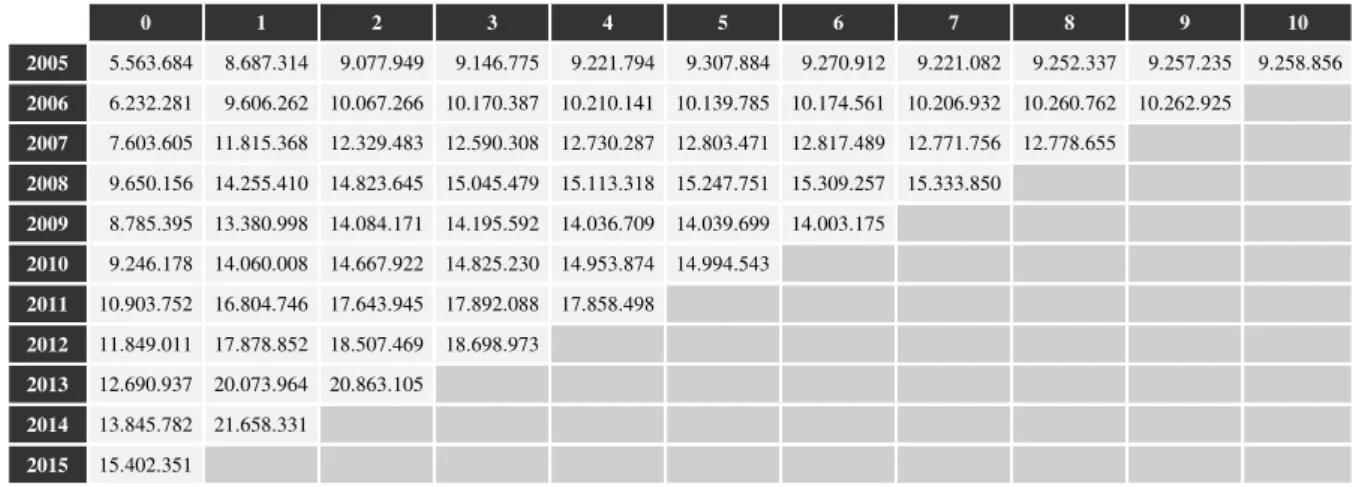
Table 2 Accumulated paid amounts ... 29

Table 3 Development factors ... 29

Table 4 Full triangle projected... 30

Table 5 Future payments discounted ... 30

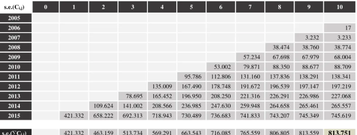
Table 6 Standard errors of the BE for WC NSLT claims provision ... 30

Table 7 Best estimate for WC NSLT claims provision ... 30

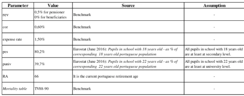
Table 8 Assumptions for WC SLT - Pensions ... 31

Table 9 Approach based on EIOPA simplification ... 33

Table 10 Approach based on EIOPA simplification - Pattern ... 33

Table 11 Approach based on EIOPA simplification - Payments per development year 33 Table 12 Extension of Mack’s model to future exposure - development factors ... 33

Table 13 Extension of Mack’s model to future exposure - accumulated costs ... 33

Table 14 Extension of Mack’s model to future exposure - (𝒔. 𝒆. (𝑪̂𝟏𝟏,𝒌)) 𝟐 ... 33

Table 15 Extension of Mack’s model to future exposure - future claims undiscounted 33 Table 16 Extension of Mack’s model to future exposure - future claims discounted .... 33

Table 17 Future claims SLT - Pensions... 34

Table 18 Future claims SLT - Lifetime assistance ... 34

Table 19 BE for premium provision ... 34

Table 20 Discount rate - impact analysis... 35

(11)

JOÃO CARVALHO

Table 22 1st assumption verification ... 40

Table 23 2nd assumption - order and classification of development factors ... 41

Table 24 2nd assumption - binomial distributions ... 41

Table 25 2nd assumption verification ... 41

Table 26 Pensions redeemable factors... 45

(12)

JOÃO CARVALHO

List of Figures

(13)

INTRODUCTION JOÃO CARVALHO

Introduction

This report is the result of an internship that I carried out from February 2016 to June 2016 at EY Portugal. As a member of the actuarial team, I had the opportunity to apply what I have learned in my master_{’s degree in real projects}, working alongside experienced actuaries and facing the diversified challenges and dynamics of a global organization. During my internship program, I was integrated in several tasks concerning audit assignments and actuarial valuation of the technical provisions for several insurers under Solvency II. Initially, I started to take knowledge of the particularities specific at each line of business and the Workers’ Compensation line of business attracted my attention in particular. This was due to three main reasons:

I. Its diversified and complex risk exposures; II. It is a mandatory policy that is highly regulated; III. It is composed of life and non-life techniques.

With this in mind, I consider that an analysis of the Workers’ Compensation line of business represents a challenge and the possibility to explore a theme that gives me an overview of both life and non-life actuarial methodologies.

Therefore, this report presents a practical analysis of the Workers’ Compensation best estimate under Solvency II and its particularities strongly regulated and specified at the Law 98/2009.

Firstly, an overview of the Workers’ Compensation liabilities and the best estimate under Solvency II is presented. Afterwards, the Workers’ Compensation best estimate under Solvency II is analysed and divided into three categories:

I. BE for WC NSLT claims provision; II. BE for WC SLT;

III. BE for premium provision.

(14)

CHAPTER 1.OVERVIEW JOÃO CARVALHO

1. Overview

1.1. W

orkers’ Compensation

Beginning in the late 1800s, many countries in Europe adopted laws to protect the employees from work-related accidents. Under Chancellor Otto von Bismark_’s command, Germany was the pioneer country and became a model for the industrialized world. An example is the “Workman’s Compensation Act.” model adapted in 1897 by the UK. Since 1913, employers in Portugal have the legal obligation to take over work-related accidents costs.

Nowadays, Workers’ Compensation (WC) program provides coverage for two types: work-related injuries and occupational illnesses (contracted as a natural incident of a repeated exposure that the worker is subject to). This program differs substantially from voluntary to mandatory systems and in most European countries (the exceptions are Belgium, Denmark, Finland, Norway and Portugal) these liabilities are managed by their national social security. In Portugal, WC program is mandatory for the employers however its liabilities are covered by nature distinct entities: the work-related injuries are insured by undertakings while the occupational illnesses are managed by the national social security. It is strongly regulated (Law 98/2009) to safeguard the beneficiaries, with a fully detailed specification of all benefits and liabilities.

(15)

medical assistance or prostheses replacement/maintenance over the lifetime of the injured worker, constitute the SLT liabilities in kind.

Despite having liabilities similar to life insurance, WC is present in the Portuguese market as a non-life business, representing 15,4% of the total with an impressive 107,3% loss ratio in 2016.

WC insurance is one of the most interesting lines of business to analyse due to its liabilities’ diversity and the high loss ratio currently in the Portuguese market. These levels of loss ratios are higher than normal and stem from a situation of technical imbalance that has persisted since the financial crisis, driven by the contraction of demand (due to the reduction of national economic activity) and strong competition between insurance companies (aggressive pricing practices in order to avoid losing market share).

1.2. Best estimate under Solvency II

Solvency II’s best estimate represents the expected present value of all the future cash flows related to the past, present and future exposure of the existing contractual obligations. These cash flows are composed of all claims payments, allocated expenses to the claims, unallocated expenses and the expected future premiums related to policies in force. The best estimate should be obtained by taking into account the uncertainty and the variability of future cash flows, calculated without any prudence margin, using realistic assumptions and applying relevant actuarial methods complemented with an adequate level of expert judgment.

Regarding the appropriateness of the data, the actuary should apply necessary adjustments to the historical data in order to increase the credibility and the quality of the projections. The time value of money should be taken into account by applying the risk free interest rates that EIOPA prescribes. The discount factor is no longer a constant value over time and it should also be applied to the WC NSLT claims provision.

(16)

I. The best estimate for claims provision is composed of the reserve related to incurred claims, including the IBNR and IBNER. This is the expected future cash flows related to the payment of claims that have already occurred. II. The best estimate for premium provision is the expected present value of the

cash flows related to future claims events of the existing contracts and, subject to some conditions (related to the definition of the contract boundary, i.e. where the undertaking has the unilateral right to cancel the contract or to reject/change the premium), renewals of existing contracts may also be included in the projection. This provision should take into account the expected profits in the future premiums and, consequently, the best estimate for premium provision might be negative.

The best estimate for life insurance obligations should be calculated separately for each policy, projecting the cash flows separately. Whenever the calculation policy by policy represents an undue burden on the insurer, projections can be made by grouping policies only if there are homogeneous risk groups, with no significant differences in the nature, and insurer obtains approximately the same results for the best estimate.

Moreover, the best estimate is calculated gross of reinsurance. The reinsurance best estimate is calculated separately under the same principles applied to the gross best estimate and it is included on the assets side of the balance sheet after having taken into account the counterparty default adjustment (expected losses due to the default of the counterparty).

(17)

CHAPTER 2.BEST ESTIMATE FOR WCNSLT CLAIMS PROVISION JOÃO CARVALHO

2. Best estimate for WC NSLT claims provision

Workers’ Compensation NSLT liabilities are mainly composed of medical expenses and temporary compensation of the salary. In this chapter, it is presented and explained the Thomas Mack’s model, one of the most recognised methodologies to estimate the claims provision in respect to liabilities non similar to life techniques. There has been quite a number of literatures about this method therefore we will provide only a brief description of it. A more detailed analysis of this methodology and its respective proofs can be found in _{Mack’s papers}mentioned in our references.

Mack’s model appears for the first time in 1993 with the main goal of measuring the variability of the Chain-Ladder estimation. A confidence interval of the estimation is of great importance for the actuary to understand the existing error under the projection made. Chain-Ladder is an intuitive methodology that does not have a probability distribution for the data, calculated using the average of the individual development factors between j-1 and j, with j=0,1,…,n. Therefore, for the development year j, the

modification rate of the payments settlement is given by,

𝑓̂𝑗=∑ 𝐶𝑖,𝑗+1

𝑛−𝑗−1 𝑖=0

∑𝑛−𝑗−1𝑖=0 𝐶𝑖,𝑗

, 𝑗 = 0,1, … , 𝑛 − 1

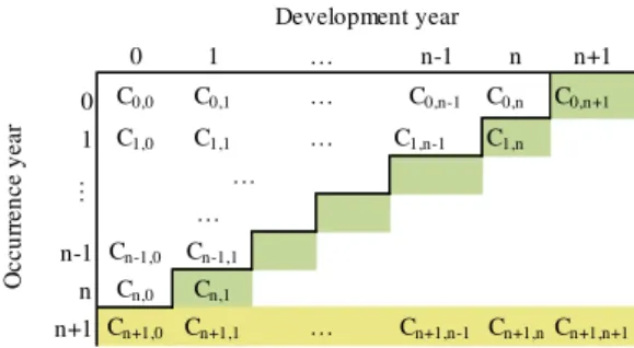
where _𝐶_𝑖,𝑗 represents the accumulated claims paid amount (including allocated loss adjustment expenses) after j years regarding to accidents occurred in year i:

Figure 1 Run off triangle

A tail factor should be implemented by the actuaries when they expect that the development years considered in the run-off triangle end before all the claims are settled. Thomas Mack suggested that the tail factor might be a linear extrapolation of ln⁡(𝑓̂𝑘− 1)

by straight line 𝑎 ∗ 𝑘 + 𝑏, 𝑎 < 0,⁡together with 𝑓̂𝑡𝑎𝑖𝑙= ∏∞𝑘=𝑛𝑓̂𝑘. Alternative methodologies to

estimate the tail factor and its standard error can be found at CAS Tail Factor Working Party, “The estimation of loss development tail factors: A summary report” in Casualty Actuarial Society E-Forum, 2013. It is important to mention that the tail factor selected

0 1 n-1 n 0 C0,0 C0,1 C0,n-1 C0,n

1 C1,0 C1,1 C1,n-1

n-1 Cn-1,0 Cn-1,1

n Cn,0

…

O

cc

u

rr

en

ce

y

ea

r

Development year

… …

(18)

and its errors must be chosen taking into account a personal assessment of the future development factors by the actuary.

Using the development factors presented above and the historical data available, the future expected payments are:

𝐶̂𝑖,𝑗= 𝐶𝑖,𝑛−𝑖∗ ∏ 𝑓̂ℎ⁡ 𝑗−1

ℎ=𝑛−𝑖

⁡, 0 ≤ 𝑖 ≤ 𝑛, 0 ≤ 𝑗 ≤ 𝑛, 𝑖 + 𝑗 > 𝑛⁡and⁡𝐶̂𝑖,𝑡𝑎𝑖𝑙= 𝐶̂𝑖,𝑛∗ 𝑓̂𝑡𝑎𝑖𝑙⁡𝑖𝑓⁡𝑎⁡𝑡𝑎𝑖𝑙⁡𝑓𝑎𝑐𝑡𝑜𝑟⁡𝑖𝑠⁡𝑎𝑝𝑝𝑙𝑖𝑒𝑑

Under Solvency II, claims provision is also discounted. For this reason, the payments must be converted to incremental values with the aim of applying the EIOPA risk free interest rates to obtain the present value of the payments.

Thus, the best estimate for the claims provision is the sum of all expected present value of future cash flows:

𝐸[𝑅] = ∑ ∑ (_{(1 + 𝑟}𝐶̂𝑖,𝑗− 𝐶̂𝑖,𝑗−1

𝑗−𝑛+𝑖)𝑗−𝑛+𝑖−0,5) 𝑛

𝑗=𝑛+1−𝑖 𝑛

𝑖=1

+ 𝐼 ∗ ∑_{(1 + 𝑟}𝐶̂𝑖,𝑡𝑎𝑖𝑙− 𝐶̂𝑖,𝑛

𝑖+1)𝑖+0,5 𝑛

𝑖=0

Where 𝐼 = {1, 𝑖𝑓⁡𝑎⁡𝑡𝑎𝑖𝑙⁡𝑓𝑎𝑐𝑡𝑜𝑟⁡𝑖𝑠⁡𝑎𝑝𝑝𝑙𝑖𝑒𝑑_{0⁡⁡⁡⁡⁡⁡⁡⁡⁡⁡⁡⁡⁡⁡⁡⁡⁡⁡⁡⁡⁡⁡⁡⁡⁡⁡⁡⁡⁡, 𝑜𝑡ℎ𝑒𝑟𝑤𝑖𝑠𝑒}

As mentioned before, the Mack’s model appears with the main goal of obtaining a confidence interval for the projection presented above. This model is based in the following three assumptions:

1. 𝐸[𝐶𝑖,𝑗+1|𝐶𝑖,𝑗] = 𝑓𝑗∗ 𝐶𝑖,𝑗, 𝑖 = 0, … , 𝑛⁡𝑎𝑛𝑑⁡𝑗 = 0, … , 𝑛 − 1

And 𝐸[𝐶𝑖,𝑡𝑎𝑖𝑙|𝐶𝑖,𝑛] = 𝑓𝑡𝑎𝑖𝑙∗ 𝐶𝑖,𝑛, 𝑖 = 0, … , 𝑛⁡𝑖𝑓⁡𝑎⁡𝑡𝑎𝑖𝑙⁡𝑓𝑎𝑐𝑡𝑜𝑟⁡𝑖𝑠⁡𝑎𝑝𝑝𝑙𝑖𝑒𝑑

2. {𝐶𝑖,1, 𝐶𝑖,2, … , 𝐶𝑖,𝑛, 𝐼 ∗ 𝐶𝑖,𝑡𝑎𝑖𝑙⁡}⁡𝑎𝑛𝑑⁡{𝐶𝑗,1, 𝐶𝑗,2, … , 𝐶𝑗,𝑛, 𝐼 ∗ 𝐶𝑗,𝑡𝑎𝑖𝑙}⁡𝑎𝑟𝑒⁡𝑖𝑛𝑑𝑒𝑝𝑒𝑛𝑑𝑒𝑛𝑡𝑠⁡𝑤ℎ𝑒𝑛⁡𝑖 ≠ 𝑗

3. 𝑉𝑎𝑟[𝐶𝑖,𝑗+1|𝐶𝑖,𝑗] = 𝐶𝑖,𝑗∗ 𝜎𝑗2⁡, 𝑖 = 0, … , 𝑛⁡𝑎𝑛𝑑⁡𝑗 = 0, … , 𝑛 − 1

where _𝜎_𝑗2₌ 1

𝑛−𝑗−1∗ ∑ 𝐶𝑖,𝑗∗ (

𝐶𝑖,𝑗+1 𝐶𝑖,𝑗 − 𝑓̂𝑗)

2

, 𝑗 = 0,1, … , 𝑛 − 2

𝑛−𝑗−1

𝑖=0 ⁡⁡

𝜎𝑛−12 = 𝑚𝑖𝑛 (𝜎𝑛−2 4

𝜎𝑛−32 , min⁡(𝜎𝑛−3

2 _{, 𝜎}

𝑛−22 ))⁡

And 𝑉𝑎𝑟[𝐶𝑖,𝑡𝑎𝑖𝑙|𝐶𝑖,𝑛] = 𝐶𝑖,𝑛∗ 𝜎𝑡𝑎𝑖𝑙2 ⁡𝑖𝑓⁡𝑎⁡𝑡𝑎𝑖𝑙⁡𝑓𝑎𝑐𝑡𝑜𝑟⁡𝑖𝑠⁡𝑎𝑝𝑝𝑙𝑖𝑒𝑑

Where 𝜎𝑡𝑎𝑖𝑙2 ⁡𝑚𝑖𝑔ℎ𝑡⁡𝑏𝑒⁡𝑎𝑛⁡𝑎𝑝𝑝𝑟𝑜𝑥𝑖𝑚𝑎𝑡𝑖𝑜𝑛⁡𝑡𝑎𝑘𝑖𝑛𝑔⁡𝑖𝑛𝑡𝑜⁡𝑎𝑐𝑐𝑜𝑢𝑛𝑡⁡𝑡ℎ𝑎𝑡⁡𝑖𝑓⁡𝑓̂𝑘−1≥ 𝑓̂𝑡𝑎𝑖𝑙≥

𝑓̂𝑘⁡𝑡ℎ𝑒𝑟𝑒𝑓𝑜𝑟𝑒⁡𝜎𝑘−12 ≥ 𝜎𝑡𝑎𝑖𝑙2 ≥ 𝜎𝑘2, 0 ≤ 𝑘 ≤ 𝑛 − 1.⁡

(19)

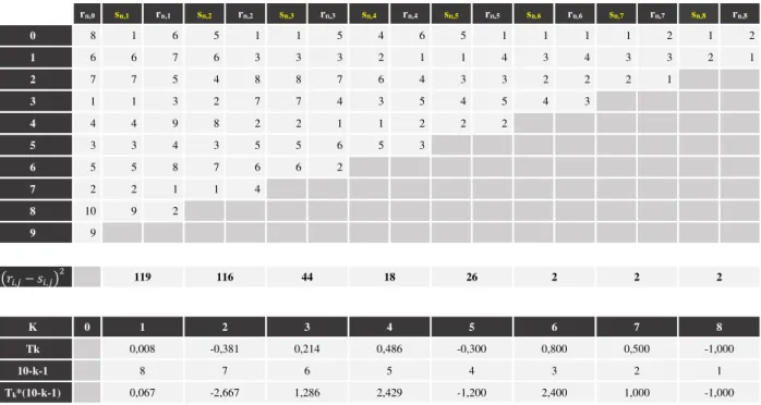
1. The 1st assumption implies that there is no correlation between the development factors. To verify this condition, it is applied the Spearman test that consists firstly in sort by ascending order, for a fixed year j, the development factors and denote their order number by 𝑟𝑖,𝑗, 1 ≤ 𝑟𝑖,𝑗≤ 𝑛 − 𝑗. After that, similarly, it is sorted the

precedent development factors ( 𝐶𝑖,𝑗

𝐶𝑖,𝑗−1), where the last value is disregarded, and then

denoting by 𝑠𝑖,𝑗, 1 ≤ 𝑠𝑖,𝑗≤ 𝑛 − 𝑗 the respective order number.

The Pearson’s coefficient, _𝑇_𝑗, is given by

𝑇𝑗= 1 − 6 ∗ ∑ (𝑟𝑖,𝑗− 𝑠𝑖,𝑗) 2

((𝑛 − 𝑗)3_{− 𝑛 + 𝑗)}⁡⁡⁡, 1 ≤ 𝑗 ≤ 𝑛 − 2⁡and − 1 ≤ 𝑇𝑗≤ 1 𝑛−𝑗−1

𝑖=0

If there is no correlation between the development factors, then 𝐸[𝑇𝑗] =

0⁡𝑎𝑛𝑑⁡𝑉𝑎𝑟(𝑇𝑗) =_{𝑛−𝑗−1}1 .

In order to apply Mack’s model, the aim is to know if the assumption is verified for the triangle as a whole and not for every pair. Thus, the formal test for the overall triangle is given by,

𝑇 = ∑_{(𝑛 − 1) ∗ (𝑛 − 2)}𝑛 − 𝑗 − 1 2

𝑛−2

𝑗=1

∗ 𝑇𝑗

Intuitively there is no correlation when 𝐸[𝑇] = 0⁡𝑎𝑛𝑑⁡𝑉𝑎𝑟(𝑇) =(𝑛−1)∗(𝑛−2)1 2

.

As the distribution of each 𝑇𝑗, 𝑛 − 𝑗 ≥ 10 can be approximated to the Normal

distribution and because T results from aggregating several uncorrelated Tk’s, we

can assume that T might be approximated to the Normal distribution. Due to the test be only an approximation and the goal is to detect correlations in substantial parts, a 50% confidence interval instead of the 95% normally applicable is used:

− 0,67

√(𝑛 − 1) ∗ (𝑛 − 2)₂

≤ 𝑇 ≤ + 0,67

√(𝑛 − 1) ∗ (𝑛 − 2)₂

When T is not within the interval, the assumption is not verified and might be better to use alternative methods to calculate the best estimate for claims provision. 2. The 2nd assumption represents the independency between different accident years.

A closer look to this condition reveals that the development factors 𝑓̂𝑗, 0 ≤ 𝑗 ≤ 𝑛 − 1

should be unbiased.

To test whether the development factors are unbiased, a stochastic test is proposed. An occurrence in a certain year affects its diagonal 𝐷𝑗= {𝐶𝑗,0, 𝐶𝑗−1,1, 𝐶𝑗−2,2, … , 𝐶0,𝑗}, 0 ≤

(20)

𝐶𝑗−1= {𝐶_𝐶𝑗−1,1_𝑗−1,0,_𝐶𝐶𝑗−2,2_𝑗−2,1, … ,_𝐶𝐶_0,𝑗−10,𝑗 }. After that, we split the development factors in two groups

(smaller and larger) and then check if one of the groups prevails. For this purpose, it is order for every j,0 ≤ 𝑗 ≤ 𝑛 − 1, 𝐹𝑗= {𝐶𝑖,𝑗+1_𝐶_𝑖,𝑗 |0 ≤ 𝑖 ≤ 𝑛 − 1 − 𝑗} that contains all

development factors between the years j and j+1. Once each 𝐹𝑗 is formed, it is

subdivided into two types: the larger factors, 𝐿𝐹𝑗, and the smaller factors, 𝑆𝐹𝑗 that

contains the elements greater/smaller than the median of 𝐹𝑗, respectively. When 𝐹𝑗

has an odd number of elements, there is a value equal to the median which is excluded. With the subdivision made, all development factors are associated to the smaller set 𝑆 = 𝑆𝐹0+ ⋯ + 𝑆𝐹𝑛−2, to the larger set 𝐿 = 𝐿𝐹0+ ⋯ + 𝐿𝐹𝑛−2 or to the eliminated

set. Intuitively, every not eliminated development factor has a probability of 50% to belong to S or L. Once classified, it should be analysed if there are diagonals where smaller/larger factors prevail. If there is a relation between accident years, it is expected that each diagonal will have approximately the same number of S and L. However, if 𝑍𝑗= min⁡(𝐿𝑗, 𝑆𝑗) is significantly smaller than 𝐿𝑗+𝑆₂ 𝑗 there is an influence

between different accident years and the assumption is not verified. To test this, it is proposed that _𝑍_𝑗 follows a probability distribution where each development factor has 50% of probability of belonging to L or S. Each 𝐿𝑗and 𝑆𝑗 follows a binomial

distribution with parameters 𝑛̀ = 𝐿𝑗+ 𝑆𝑗 and 𝑝 = 0,5. Thus, assuming that 𝑚 =𝑛̀−1₂

denotes the largest integer ≤𝑛̀−1₂ ,

𝐸[𝑍𝑗] =𝑛̀₂− (𝑛̀ − 1_𝑚 ) ∗₂𝑛̀𝑛̀

𝑉𝑎𝑟(𝑍𝑗) =𝑛̀ ∗ (𝑛̀ − 1)₄ − (𝑛̀ − 1_𝑚 ) ∗𝑛̀ ∗ (𝑛̀ − 1)₂_𝑛̀ + 𝐸[𝑍𝑗] − 𝐸2[𝑍𝑗]

Our goal is to test the overall 𝑍 = 𝑍1+ ⋯ + 𝑍𝑛−1. As under the null-hypothesis the

different 𝑍𝑗′𝑠 are uncorrelated1 and assuming that Z is approximately a Normal

distribution, the assumption is not verified with a 95% confidence interval if Z is not contained within the interval

𝐸[𝑍] − 1,96 ∗ √𝑉𝑎𝑟(𝑍) ≤ 𝑍 ≤ 𝐸[𝑍] + 1,96 ∗ √𝑉𝑎𝑟(𝑍)

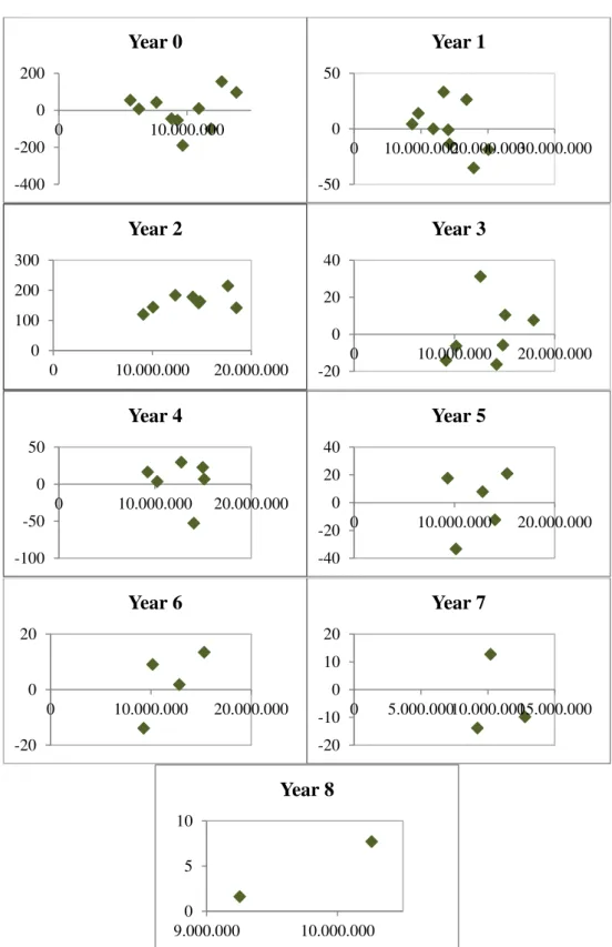
3. Interpreting the 3rd assumption, the conditional variance of 𝐶𝑖,𝑗+1 is directly

proportional to 𝐶𝑖,𝑗 with a constant factor 𝜎𝑗2. Therefore, if the assumption is verified,

the weighted residual is given by,

(𝐶𝑖,𝑗+1− 𝐶𝑖,𝑗∗ 𝑓̂)𝑗 2≈ 𝐶𝑖,𝑗∗ 𝜎𝑗2⁡𝑤ℎ𝑖𝑐ℎ⁡𝑖𝑠⁡𝑒𝑞𝑢𝑖𝑣𝑎𝑙𝑒𝑛𝑡⁡𝑡𝑜⁡𝜎𝑗≈𝐶𝑖,𝑗+1−𝐶𝑖,𝑗∗𝑓𝑗 ̂ √𝐶𝑖,𝑗 ⁡

1_{𝐸[𝑍] = 𝐸[𝑍}

(21)

Under the assumption, it is expected that there is no relation between the weighted residual and 𝐶𝑖,𝑗. In order to conclude if the assumption is verified, we should plot

all pairs (𝐶𝑖,𝑗+1−𝐶𝑖,𝑗∗𝑓̂𝑗

√𝐶𝑖,𝑗 , 𝐶𝑖,𝑗) and observe if they are purely random without a specific

trend. When a trend is observable, it is recommendable to use alternative development factors or even not to apply this method.

With the assumptions now explained, it is time to present the variability associated to the estimation. Based in the assumptions above, Thomas Mack has derived that the standard error of 𝐶̂𝑖,𝑗 is gathered in the following recursive formula with a starting point (𝑠. 𝑒. (𝐶̂𝑖,𝑛−𝑖))2= 0,

(𝑠. 𝑒. (𝐶̂𝑖,𝑗+1))2= (𝐶̂𝑖,𝑗)2∗ ((𝑠. 𝑒. (𝐹̂𝑖,𝑗)) 2

+ ⁡(𝑠. 𝑒. (𝑓̂̇𝑗)) 2

) + (𝑠. 𝑒. (𝐶̂𝑖,𝑗))2∗ 𝑓̂̇𝑗 2

Where

⁡(𝑠. 𝑒. (𝑓̂𝑗)) 2

= 𝜎̂𝑗2 ∑𝑛−𝑗−1𝑘=0 𝐶𝑘,𝑗

⁡⁡𝑎𝑛𝑑⁡⁡ (𝑠. 𝑒. (𝐹̂𝑖,𝑗)) 2

=𝜎̂𝑗2

𝐶̂𝑖,𝑗⁡, 0 ≤ 𝑖 ≤ 𝑛⁡𝑎𝑛𝑑⁡0 ≤ 𝑗 ≤ 𝑛 − 1

Intuitively the standard error for the occurrence year i, simultaneously equivalent to the standard error of the estimated reserve 𝑅̂𝑖= 𝐶̂𝑖,𝑛− 𝐶𝑖,𝑛−𝑖, is given by

(𝑠. 𝑒. (𝐶̂𝑖,𝑛))2= (𝐶̂𝑖,𝑛)2∗ ∑

(𝑠. 𝑒. (𝐹̂𝑖,𝑘)) 2

+ ⁡(𝑠. 𝑒. (𝑓̂̇𝑘)) 2

𝑓̂𝑘2 𝑛−1

𝑘=𝑛−𝑖

If a tail factor is included the equation is automatically extended to

(𝑠. 𝑒. (𝐶̂𝑖,𝑡𝑎𝑖𝑙))2= (𝐶̂𝑖,𝑡𝑎𝑖𝑙)2∗ ((𝑠. 𝑒. (𝐹̂𝑖,𝑡𝑎𝑖𝑙)) 2

+ ⁡(𝑠. 𝑒. (𝑓̂̇𝑡𝑎𝑖𝑙)) 2

) + (𝑠. 𝑒. (𝐶̂𝑖,𝑛))2∗ 𝑓̂̇𝑡𝑎𝑖𝑙 2

Where (𝑠. 𝑒. (𝐹̂𝑖,𝑡𝑎𝑖𝑙)) 2

⁡and⁡⁡(𝑠. 𝑒. (𝑓̂̇𝑡𝑎𝑖𝑙)) 2

might⁡be⁡approximated⁡taking⁡into⁡account⁡that⁡if⁡𝑓̂𝑘−1≥

𝑓̂𝑡𝑎𝑖𝑙≥ 𝑓̂𝑘⁡therefore⁡ (𝑠. 𝑒. (𝐹̂𝑖,𝑘−1)) 2

≥ (𝑠. 𝑒. (𝐹̂𝑖,𝑡𝑎𝑖𝑙)) 2

≥ (𝑠. 𝑒. (𝐹̂𝑖,𝑘)) 2

⁡and⁡⁡(𝑠. 𝑒. (𝑓̂̇𝑘−1)) 2

≥

⁡(𝑠. 𝑒. (𝑓̂̇𝑡𝑎𝑖𝑙)) 2

≥ ⁡(𝑠. 𝑒. (𝑓̂̇𝑘)) 2

, 0 ≤ 𝑘 ≤ 𝑛 − 1

Moreover, it is equally important to determine the standard error of the overall ultimate

∑ 𝐶̂𝑛𝑖=0 𝑖,𝑛𝑡𝑎𝑖𝑙where⁡ntail = { 𝑡𝑎𝑖𝑙⁡, if⁡a⁡tail⁡factor⁡is⁡applied_{𝑛,⁡⁡⁡⁡⁡⁡⁡⁡⁡⁡⁡⁡⁡⁡⁡⁡⁡⁡⁡⁡⁡⁡⁡⁡⁡⁡⁡⁡⁡⁡⁡⁡⁡⁡⁡otherwise}. In this case, we cannot simply sum all

(𝑠. 𝑒. (𝐶̂𝑖,𝑛𝑡𝑎𝑖𝑙))2, 0 ≤ 𝑖 ≤ 𝑛, because they are correlated through common factors 𝑓̂̇𝑗⁡and⁡𝜎̂𝑗2.

(22)

reserve can be estimated when 𝑗 = { 𝑛⁡𝑖𝑓⁡𝑛𝑡𝑎𝑖𝑙 = 𝑡𝑎𝑖𝑙_{𝑛 − 1⁡𝑖𝑓⁡𝑛𝑡𝑎𝑖𝑙 = 𝑛} , where n+1=tail and 𝑓̂𝑛2= 𝑓̂𝑡𝑎𝑖𝑙2 in the

following recursive formula with a starting point j=0,

(𝑠. 𝑒. (∑𝑛𝑖=𝑛−𝑗𝐶̂𝑖,𝑗+1)) 2

= ∑ (𝐶̂𝑖,𝑗)2∗ (𝑠. 𝑒. (𝐹̂𝑖,𝑗)) 2 𝑛

𝑖=𝑛−𝑗 + (∑𝑛𝑖=𝑛−𝑗𝐶̂𝑖,𝑗)2∗ ⁡(𝑠. 𝑒. (𝑓̂̇𝑗))

2

+

+ (𝑠. 𝑒. (∑𝑛𝑖=𝑛−𝑗+1𝐶̂𝑖,𝑗)) 2

∗ 𝑓̂𝑗2

When the volume of the outstanding claims is large enough, it is possible to construct a confidence interval taking into account the central limit theorem. The symmetric 95%-confidence interval is given by ]𝐸[𝑅] − 1,96 ∗ 𝑠. 𝑒. (∑ 𝐶̂𝑛𝑖=0 𝑖,𝑛𝑡𝑎𝑖𝑙); 𝐸[𝑅] + 1,96 ∗ 𝑠. 𝑒. (∑ 𝐶̂𝑛𝑖=0 𝑖,𝑛𝑡𝑎𝑖𝑙)[

(23)

CHAPTER 3.BEST ESTIMATE FOR WCSLT JOÃO CARVALHO

3. Best estimate for WC SLT

As previously mentioned, WC SLT liabilities are composed of pensions and lifetime assistance payments:

a. Pensions are split into disability pensions when the worker suffers an accident restricting his/her ability to work in a permanent way and pensions for dependants on the death of the insured. It is important to refer that some pensions can be redeemable if some conditions are fulfilled.

b. Lifetime assistance is composed mainly by permanent medical assistance payments or prostheses replacement over the lifetime of the injured worker. Even though it is not included in our analysis, it is worth noting that insurers should also make an annual contribution based on the capital redemption relating to pensions in payment to the Workers’ Compensation Fund managed by ASF.

WC SLT liabilities should be calculated case-by-case for the whole portfolio. Due to the diversity and the different exposure to risk, non-redeemable pensions, redeemable pensions and lifetime assistance should be analysed separately as presented below.

3.1. Non-redeemable pensions

Pensions are calculated on an annuity basis, payable monthly and adding two extra allowances: for holidays in July and for Christmas in November.

According to Portuguese law, the pension value can be revised one-time per civil year without time limit and can be requested by the policyholder or the undertaking. If the workers’ incapacity has changed through the year, the pension value is adapted in accordance with the current incapacity.

(24)

stage, its provision includes a correction rate calculated taking into account the past experience.

Moreover, for the pensions’ calculation purposes, we have the following categories:

 Fully disabled to perform any kind of work

Lifelong pension of 80% worker’s wage plus 10% for each dependant limited to worker’s wage.

 Fully disabled for the usual work

Lifelong pension from 50% to 70% of the wage, depending on the _workers’ capability to execute other type of job.

 Partial permanent incapacity

Lifelong pension equals to 70% of the reduction in the wage.

 Pensions for the worker’s dependants in case of death

The main beneficiaries of these pensions are spouses or equivalent, descendants and ascendants. A detailed description of which people are recognized in each category is found in Law 98/2009.

The main pensions2_{paid in case of death are the following (all pensions are}

calculated proportionally to the worker_’s annual wage):

- Spouse or equivalent: 30% until the normal retirement age and after that

increases to 40%.

- Descendants: 20% if there is one descendant, 40% if there are two descendants and 50% if there are three or more descendants. These pensions are paid until they complete 18 years old. The payment period must be extended until they complete 22 years old if they are at least at the secondary school level or 25 years if they are at the university level. All pensions should be adjusted if the number of descendants’ beneficiaries changes. If a descendant suffers from any significant (75% or more) permanent disability

2_{It was excluded the case when the undertaking has to continue to pay a maintenance allowance for an ex-spouse when she/he had}

(25)

to work or has a significant chronic disease, he/she receives the pension for the whole life. All of these pensions can double (with a max value of 80% of the annual worker’s wage) if the other parent also dies.

- Ascendants: 10% for each ascendant until a maximum of 30%. If there are

no others beneficiaries, they receive 15% each until retirement age or until a chronic disease appears and 20% after that.

- FAT: If the worker who died has no dependants, the undertaking should revert to the FAT three times his/her annual wage.

The sum of all retributions above cannot exceed 80% of the annual wage of the dead worker. If this happens, the retributions should be proportionally revised to not exceed this limit.

Therefore, below we present the best estimate for each process and methodologies to calculate the best estimate for each type of pension when it is not redeemable (explained posteriorly):

𝑃𝑃𝑉 = {_{𝑎 ∗ (1 + 𝑐𝑜𝑟) ∗ (𝑃𝑃𝑉}3 ∗ 𝑤⁡⁡⁡⁡⁡⁡⁡⁡⁡⁡⁡⁡⁡⁡⁡⁡⁡⁡⁡⁡⁡⁡⁡⁡⁡⁡⁡⁡⁡⁡⁡⁡⁡⁡⁡⁡⁡⁡⁡⁡⁡⁡⁡⁡⁡⁡⁡⁡⁡⁡⁡⁡⁡⁡⁡⁡⁡⁡⁡⁡⁡⁡⁡⁡⁡⁡⁡⁡⁡⁡⁡⁡⁡⁡⁡⁡⁡⁡⁡⁡⁡⁡⁡⁡⁡⁡⁡⁡⁡⁡⁡⁡⁡⁡⁡⁡⁡⁡⁡⁡⁡⁡⁡⁡⁡⁡⁡⁡⁡⁡⁡⁡⁡⁡⁡⁡⁡⁡⁡⁡⁡⁡⁡⁡⁡⁡⁡⁡𝑖𝑓⁡𝑎 = 0^𝑑 = 0

𝑤𝑜𝑟𝑘𝑒𝑟) + (1 − 𝑎) ∗ (𝑃𝑃𝑉𝑠+ 𝑃𝑃𝑉𝑑𝑒𝑠𝑐+ 𝑃𝑃𝑉𝑎𝑠𝑐)⁡⁡⁡⁡⁡⁡⁡⁡⁡⁡⁡𝑜𝑡ℎ𝑒𝑟𝑤𝑖𝑠𝑒⁡⁡⁡⁡⁡⁡⁡⁡⁡⁡⁡⁡⁡⁡

Where,

𝑤 = 12 ∗ 𝑚𝑜𝑛𝑡ℎ𝑙𝑦⁡𝑤𝑎𝑔𝑒⁡𝑜𝑓⁡𝑡ℎ𝑒⁡𝑤𝑜𝑟𝑘𝑒𝑟⁡𝑤ℎ𝑒𝑛⁡𝑡ℎ𝑒⁡𝑎𝑐𝑐𝑖𝑑𝑒𝑛𝑡⁡ℎ𝑎𝑝𝑝𝑒𝑛𝑠 ∗ (1 + 𝑒𝑥𝑝𝑒𝑛𝑠𝑒⁡𝑟𝑎𝑡𝑒)

𝑎 = ⁡ { 0⁡𝑖𝑓⁡𝑡ℎ𝑒⁡𝑤𝑜𝑟𝑘𝑒𝑟⁡𝑑𝑖𝑒𝑑_{1⁡𝑖𝑓⁡𝑡ℎ𝑒⁡𝑤𝑜𝑟𝑘𝑒𝑟⁡𝑖𝑠⁡𝑎𝑙𝑖𝑣𝑒}

𝑑 = 𝑛𝑢𝑚𝑏𝑒𝑟⁡𝑜𝑓⁡𝑑𝑒𝑝𝑒𝑛𝑑𝑎𝑛𝑡𝑠

𝑐𝑜𝑟⁡𝑖𝑠⁡𝑡ℎ𝑒⁡𝑐𝑜𝑟𝑟𝑒𝑐𝑡𝑖𝑜𝑛⁡𝑟𝑎𝑡𝑒.⁡⁡𝐼𝑓⁡𝑡ℎ𝑒⁡𝑝𝑒𝑛𝑠𝑖𝑜𝑛⁡𝑖𝑠⁡⁡𝑑𝑒𝑓𝑖𝑛𝑒𝑑⁡ ⇒ 𝑐𝑜𝑟 = ⁡0

𝑃𝑃𝑉𝑤𝑜𝑟𝑘𝑒𝑟= 𝑃𝑒𝑛𝑠𝑖𝑜𝑛⁡𝑃𝑟𝑒𝑠𝑒𝑛𝑡⁡𝑉𝑎𝑙𝑢𝑒⁡𝑤ℎ𝑒𝑛⁡𝑡ℎ𝑒⁡𝑤𝑜𝑟𝑘𝑒𝑟⁡𝑠𝑡𝑖𝑙𝑙⁡𝑎𝑙𝑖𝑣𝑒

𝑃𝑃𝑉𝑠= 𝑃𝑒𝑛𝑠𝑖𝑜𝑛⁡𝑃𝑟𝑒𝑠𝑒𝑛𝑡⁡𝑉𝑎𝑙𝑢𝑒⁡𝑜𝑓⁡𝑡ℎ𝑒⁡𝑠𝑝𝑜𝑢𝑠𝑒

𝑃𝑃𝑉𝑑𝑒𝑠𝑐= 𝑃𝑒𝑛𝑠𝑖𝑜𝑛⁡𝑃𝑟𝑒𝑠𝑒𝑛𝑡⁡𝑉𝑎𝑙𝑢𝑒⁡𝑓𝑜𝑟⁡𝑑𝑒𝑠𝑐𝑒𝑛𝑑𝑎𝑛𝑡𝑠

(26)

3.1.A. Worker is alive

𝑃𝑃𝑉𝑤𝑜𝑟𝑘𝑒𝑟=

{

min(0,8 + 0,1 ∗ 𝑑; 1) ∗ 𝑤 ∗ 𝑎𝑠̈𝑥(12)⁡𝑖𝑓⁡𝑤𝑜𝑟𝑘𝑒𝑟⁡𝑖𝑠⁡𝑓𝑢𝑙𝑙𝑦⁡𝑑𝑖𝑠𝑎𝑏𝑙𝑒𝑑⁡𝑓𝑜𝑟⁡𝑎𝑛𝑦⁡𝑘𝑖𝑛𝑑⁡𝑜𝑓⁡𝑤𝑜𝑟𝑘⁡(𝑓𝑑𝑘𝑤)

m ∗ 𝑤 ∗ 𝑎𝑠̈𝑥(12)⁡⁡⁡⁡⁡⁡⁡⁡⁡⁡⁡⁡⁡⁡⁡⁡⁡⁡⁡⁡⁡⁡⁡⁡⁡⁡⁡⁡⁡⁡⁡⁡⁡, 𝑖𝑓⁡𝑤𝑜𝑟𝑘𝑒𝑟⁡𝑖𝑠⁡𝑓𝑢𝑙𝑙𝑦⁡𝑑𝑖𝑠𝑎𝑏𝑙𝑒𝑑⁡𝑓𝑜𝑟⁡𝑡ℎ𝑒⁡𝑢𝑠𝑢𝑎𝑙⁡𝑤𝑜𝑟𝑘⁡(𝑓𝑑𝑢𝑤)

0,7 ∗ (w − 𝑤𝑎𝑓𝑡𝑒𝑟⁡𝑎𝑐𝑐𝑖𝑑𝑒𝑛𝑡) ∗ 𝑎𝑠̈𝑥(12)⁡⁡⁡⁡⁡⁡⁡⁡⁡⁡⁡⁡⁡⁡⁡⁡⁡⁡⁡⁡⁡⁡⁡⁡⁡, 𝑖𝑓⁡𝑤𝑜𝑟𝑘𝑒𝑟⁡𝑖𝑠⁡𝑝𝑎𝑟𝑡𝑖𝑎𝑙𝑙𝑦⁡𝑑𝑖𝑠𝑎𝑏𝑙𝑒𝑑⁡𝑓𝑜𝑟⁡𝑡ℎ𝑒⁡𝑤𝑜𝑟𝑘⁡(𝑝𝑑𝑤)

Where,

𝑚 ∈ [0,5; 0,7]⁡𝑑𝑒𝑝𝑒𝑛𝑑𝑖𝑛𝑔⁡𝑜𝑛⁡𝑡ℎ𝑒⁡𝑐𝑎𝑝𝑎𝑐𝑖𝑡𝑦⁡𝑡𝑜⁡𝑑𝑜⁡𝑎𝑛𝑜𝑡ℎ𝑒𝑟⁡𝑗𝑜𝑏

𝑎𝑠̈𝑥(12)= 𝑎̈𝑥(12)+∑ 𝑠𝑘,𝑥 ∞𝑥 𝑘=0

12

𝑎̈𝑥(12) ≈⏞ 𝑈𝐷𝐷3

13

24+ ∑ (

1+𝑟𝑒𝑣 1+𝑟𝑘)

𝑘 ∞𝑥

𝑘=1 ∗𝑙𝑥+𝑘_𝑙_𝑥

𝑠𝑘,𝑦= [𝑣𝑘+10,5+𝑘∗0,5+𝑘𝑝𝑦+ 𝑣𝑘+1 11 12+𝑘_∗₁₁

12+𝑘𝑝𝑦] ∗ (1 + 𝑟𝑒𝑣) 𝑘+1

𝑒+𝑘𝑝𝑥=𝑘𝑝𝑥∗𝑒𝑝𝑥+𝑘 ≈⏞ 𝐶𝐹𝑀4

𝑘𝑝𝑥∗ (𝑝𝑥+𝑘)𝑒⁡, 0 ≤ 𝑒 < 1

𝑣𝑘=_{(1 + 𝑟}1

𝑘) , 𝑟𝑘⁡𝑓𝑟𝑜𝑚⁡𝐸𝐼𝑂𝑃𝐴⁡𝑟𝑖𝑠𝑘⁡𝑓𝑟𝑒𝑒⁡𝑟𝑎𝑡𝑒⁡𝑖𝑛𝑡𝑒𝑟𝑒𝑠𝑡⁡𝑡𝑒𝑟𝑚⁡𝑠𝑡𝑟𝑢𝑐𝑡𝑢𝑟𝑒𝑠⁡

∞𝑥= max 𝑎𝑔𝑒⁡𝑖𝑛⁡𝑡ℎ𝑒⁡𝑚𝑜𝑟𝑡𝑎𝑙𝑖𝑡𝑦⁡𝑡𝑎𝑏𝑙𝑒 − 𝑥

𝑟𝑒𝑣 = 𝑟𝑒𝑣𝑖𝑠𝑖𝑜𝑛⁡𝑟𝑎𝑡𝑒

3.1.B. Pension for the spouse if the worker dies

Assumption: the spouse will not remarry (when this happens a lump sum retribution of three times the annual wage is paid and the pension is then cancelled)

𝑃𝑃𝑉𝑠=

{

0,3 ∗ 𝑤 ∗ 𝑎𝑠̈𝑦(12)+ 0,1 ∗ 𝑤 ∗𝑙_𝑙𝑅𝐴

𝑦 ∗ 𝑣𝑅𝐴−𝑦

𝑅𝐴−𝑦_{∗ 𝑎𝑠̈}

𝑅𝐴(12)⁡⁡⁡⁡⁡⁡⁡⁡⁡⁡⁡⁡⁡𝑖𝑓⁡𝑠𝑝𝑜𝑢𝑠𝑒⁡ℎ𝑎𝑠⁡𝑛𝑜𝑡⁡𝑟𝑒𝑡𝑖𝑟𝑒𝑑

0,4 ∗ 𝑤 ∗ 𝑎𝑠̈𝑦(12)⁡⁡⁡⁡⁡⁡⁡⁡⁡⁡⁡⁡⁡⁡⁡⁡⁡⁡⁡⁡⁡⁡⁡⁡⁡⁡⁡⁡⁡⁡⁡⁡⁡⁡⁡⁡⁡⁡⁡⁡⁡⁡⁡⁡⁡⁡⁡⁡⁡⁡⁡⁡⁡⁡⁡⁡⁡⁡⁡⁡⁡⁡⁡⁡⁡⁡⁡⁡⁡⁡⁡⁡⁡⁡𝑖𝑓⁡𝑠𝑝𝑜𝑢𝑠𝑒⁡ℎ𝑎𝑠⁡𝑎𝑙𝑟𝑒𝑎𝑑𝑦⁡𝑟𝑒𝑡𝑖𝑟𝑒𝑑

0⁡⁡⁡⁡⁡⁡⁡⁡⁡⁡⁡⁡⁡⁡⁡⁡⁡⁡⁡⁡⁡⁡⁡⁡⁡⁡⁡⁡⁡⁡⁡⁡⁡⁡⁡⁡⁡⁡⁡⁡⁡⁡⁡⁡⁡⁡⁡⁡⁡⁡⁡⁡⁡⁡⁡⁡⁡⁡⁡⁡⁡⁡⁡⁡⁡⁡⁡⁡⁡⁡⁡⁡⁡⁡𝑖𝑓⁡𝑤𝑜𝑟𝑘𝑒𝑟⁡𝑑𝑜𝑒𝑠⁡𝑛𝑜𝑡⁡ℎ𝑎𝑣𝑒⁡𝑠𝑝𝑜𝑢𝑠𝑒

Where,

_{𝑦 = 𝑠𝑝𝑜𝑢𝑠𝑒′𝑠⁡𝑎𝑔𝑒}

_{𝑅𝐴 = 𝑛𝑜𝑟𝑚𝑎𝑙⁡𝑟𝑒𝑡𝑖𝑟𝑒𝑚𝑒𝑛𝑡⁡𝑎𝑔𝑒}

3_{Under UDD approach:}_𝑎̈

𝑥 (𝑚)_{≈ 𝑎̈}

𝑥−𝑚−1_2𝑚 = ∑ (𝑣∞𝑘=0𝑥 𝑘∗𝑘𝑝𝑥) −𝑚−1_2𝑚 = 1 −𝑚−1_2𝑚+ ∑ (𝑣∞𝑘=1𝑥 𝑘∗𝑘𝑝𝑥)

4_{Constant Force of Mortality Assumption: for x integer and}_{0 ≤ 𝑒 < 1,}

(27)

3.1.C. Pensions for the descendants if the worker dies

Assumption: the descendant will not become significantly disabled to work and/or suffers from a chronic disease if he/she was healthy when he/she started receiving the pension, and will not become an orphan as well. It is also assumed that the descendants when entry to the secondary/university level, will not leave until they are 22/25 years old respectively. Moreover, when there are more than three descendants, the overall pension is allocated among the three youngest ones5_{: 20% for each of the two youngest}

descendants and the remaining 10% for the third youngest descendant (of course when both parents have died, the pension is only split for the two youngest descendants with 40% for each, due to the maximum limit retribution of 80%). This approach does not consider the case that an older descendant can remain longer than a young one if he/she studies at university level, and the younger does not. However, due to a high number of possible situations, modelling with no approaches could result in a very complex model and very difficult to apply in practice. Regarding this, the proposed methodology presents an adequate balance between the degree of complexity and the significance of all possible situations;

𝑃𝑃𝑉𝑑𝑒𝑠𝑐(𝑐)

=

{

0⁡⁡⁡⁡⁡⁡⁡⁡⁡⁡⁡⁡⁡⁡⁡⁡⁡⁡⁡⁡⁡⁡⁡⁡⁡⁡⁡⁡⁡⁡⁡⁡⁡⁡⁡⁡⁡⁡⁡⁡⁡⁡⁡⁡⁡⁡⁡⁡⁡⁡⁡⁡⁡⁡⁡⁡⁡⁡⁡⁡⁡⁡⁡⁡⁡⁡⁡⁡⁡⁡⁡⁡⁡⁡⁡⁡⁡⁡⁡⁡⁡⁡⁡⁡⁡⁡⁡⁡⁡⁡⁡⁡⁡⁡⁡⁡⁡⁡⁡⁡⁡⁡⁡⁡⁡⁡⁡⁡⁡⁡⁡⁡⁡⁡⁡⁡⁡⁡⁡⁡⁡⁡⁡⁡⁡⁡⁡⁡⁡⁡⁡⁡⁡⁡⁡⁡⁡⁡⁡⁡⁡⁡⁡⁡⁡⁡⁡⁡⁡⁡⁡⁡⁡⁡⁡⁡⁡⁡⁡⁡⁡⁡⁡⁡⁡⁡⁡⁡⁡⁡⁡⁡⁡⁡⁡⁡⁡⁡⁡⁡⁡⁡⁡⁡, 𝑐 = 0

0,4 ∗ 𝑤 ∗1_ℎ∗

[

𝐼𝑐𝑑∗ ∑ 𝑎𝑠̈_𝑧(12)_(𝑖) min(𝑐𝑑,2)

𝑖=1

+

𝐼𝑐𝑛𝑑∗ ∑ (𝑑_𝑖1∗ 𝑎𝑠̈_𝑧

(𝑖):18−𝑧̅̅̅̅̅̅̅̅̅̅̅̅(𝑖)⁡|

(12) _{+ 𝑑}

𝑖2∗ 𝑎̈𝑠𝑧(12)_(𝑖):22−𝑧̅̅̅̅̅̅̅̅̅̅̅̅_(𝑖)⁡|+ 𝑑𝑖3∗ 𝑎𝑠̈𝑧(12)_(𝑖):25−𝑧̅̅̅̅̅̅̅̅̅̅̅̅_(𝑖)⁡|) min(𝑐𝑛𝑑_,2)

𝑖=1 ]

⁡⁡⁡⁡⁡⁡⁡⁡⁡⁡⁡⁡⁡⁡⁡⁡⁡⁡⁡, 𝑐 = 1,2⁡

𝑃𝑃𝑉𝑑𝑒𝑠𝑐(2) + 0,1 ∗ (ℎ − 1) ∗ 𝑤 ∗ [

𝐷𝑧(3)∗ 𝑎𝑠̈𝑧(3)

(12)₊

(1 − 𝐷𝑧(3)) (𝑑31∗ 𝑎𝑠̈𝑧(3):18−𝑧̅̅̅̅̅̅̅̅̅̅̅̅̅(3)⁡|

(12) _{+ 𝑑}

32∗ 𝑎𝑠̈𝑧(3):22−𝑧̅̅̅̅̅̅̅̅̅̅̅̅̅(3)⁡|

(12) _{+ 𝑑}

33∗ 𝑎𝑠̈𝑧(3):25−𝑧̅̅̅̅̅̅̅̅̅̅̅̅̅(3)⁡|

(12) ₎] , 𝑐 ≥ 3

Where,

ℎ = { 1⁡, 𝑖𝑓⁡𝑡ℎ𝑒𝑦⁡𝑎𝑟𝑒⁡⁡𝑜𝑟𝑝ℎ𝑎𝑛𝑠_{2⁡, 𝑖𝑓⁡𝑡ℎ𝑒𝑦⁡𝑎𝑟𝑒⁡𝑛𝑜𝑡⁡𝑜𝑟𝑝ℎ𝑎𝑛𝑠⁡}

𝐼𝑥= { 0, 𝑖𝑓⁡𝑥 = 0_{1, 𝑜𝑡ℎ𝑒𝑟𝑤𝑖𝑠𝑒}

5_{When there are three or more descendants, it is used to split the 50% retribution uniformly for all descendants, provisioning}

independently for each descendant. However, this cannot be a reasonable approach when there is a big difference between the

beneficiaries’ age. For example, considering there are three descendants with 2, 4 and 24 years old: In this case, it would be

provisioning 16,6(6)% with maturities of 23, 21 and 1 yearrespectively (assuming that allbeneficiaries goto the university). However, if everyone survives until the maturity (it is the expected due to the high survival rates for early ages), this provision is underestimated because after the 1st_{year and for the following 20 years, the retribution will be 20% for each of the two youngest descendants and not}

(28)

𝑐𝑛𝑑_{= 𝑛𝑢𝑚𝑏𝑒𝑟⁡𝑜𝑓⁡𝑑𝑒𝑠𝑐𝑒𝑛𝑑𝑎𝑛𝑡𝑠⁡𝑛𝑜𝑡⁡𝑑𝑖𝑠𝑎𝑏𝑙𝑒𝑑}

𝑐𝑑_{= 𝑛𝑢𝑚𝑏𝑒𝑟⁡𝑜𝑓⁡𝑑𝑒𝑠𝑐𝑒𝑛𝑑𝑎𝑛𝑡𝑠⁡𝑑𝑖𝑠𝑎𝑏𝑙𝑒𝑑}

𝑐 = 𝑐𝑑_{+ 𝑐}𝑛𝑑_{= 𝑛𝑢𝑚𝑏𝑒𝑟⁡𝑜𝑓⁡𝑑𝑒𝑠𝑐𝑒𝑛𝑑𝑎𝑛𝑡𝑠}

𝑧(𝑖)= 𝑎𝑔𝑒⁡𝑜𝑓⁡𝑡ℎ𝑒⁡𝑑𝑒𝑠𝑐𝑒𝑛𝑑𝑒𝑛𝑡⁡𝑖, 𝑖𝑛⁡𝑎𝑠𝑐𝑒𝑛𝑑𝑖𝑛𝑔⁡𝑜𝑟𝑑𝑒𝑟⁡𝑎𝑛𝑑⁡𝑓𝑖𝑟𝑠𝑡𝑙𝑦⁡𝑡ℎ𝑒⁡𝑑𝑖𝑠𝑎𝑏𝑙𝑒𝑑

𝑑𝑖1= {_{0,⁡⁡⁡𝑜𝑡ℎ𝑒𝑟𝑤𝑖𝑠𝑒}1⁡,⁡⁡⁡𝑧(𝑖)< 18⁡

𝑑𝑖2=

{ 𝑝𝑒𝑠 ∗ 𝑙18

𝑙𝑧𝑖

∗ 𝑣_18−𝑧18−𝑧_𝑖𝑖_{∗ 𝑎𝑠̈} 18:4|(12)̅∗

1 𝑎𝑠̈_{𝑧(𝑖):22−𝑧(𝑖)⁡|}(12)̅̅̅̅̅̅̅̅̅̅̅̅̅

, 𝑧𝑖< 18

1⁡⁡⁡⁡⁡⁡, 18 ≤ 𝑧𝑖 < 22⁡

0⁡⁡, 𝑜𝑡ℎ𝑒𝑟𝑤𝑖𝑠𝑒

𝑑𝑖3=

{

𝑝𝑢𝑛𝑖𝑣 ∗ 𝑙22

𝑙𝑧𝑖

∗ 𝑣22−𝑧𝑖 22−𝑧𝑖_{∗ 𝑎𝑠̈}

22:3|(12)̅∗ 1

𝑎𝑠̈_{𝑧(𝑖):25−𝑧(𝑖)⁡|}(12)̅̅̅̅̅̅̅̅̅̅̅̅̅

, 𝑧𝑖< 22

1⁡⁡⁡⁡⁡⁡, 22 ≤ 𝑧𝑖 < 25⁡

0⁡⁡, 𝑜𝑡ℎ𝑒𝑟𝑤𝑖𝑠𝑒

𝑝𝑒𝑠 = 𝑝𝑟𝑜𝑏𝑎𝑏𝑖𝑙𝑖𝑡𝑦⁡𝑜𝑓⁡𝑠𝑡𝑖𝑙𝑙⁡𝑠𝑡𝑢𝑑𝑦𝑖𝑛𝑔⁡𝑤𝑖𝑡ℎ⁡18⁡𝑦𝑒𝑎𝑟𝑠⁡𝑜𝑙𝑑⁡𝑎𝑡⁡𝑠𝑒𝑐𝑜𝑛𝑑𝑎𝑟𝑦⁡𝑜𝑟⁡ℎ𝑖𝑔ℎ𝑒𝑟⁡𝑙𝑒𝑣𝑒𝑙

_{𝑝𝑢𝑛𝑖𝑣 = 𝑝𝑟𝑜𝑏𝑎𝑏𝑖𝑙𝑖𝑡𝑦⁡𝑜𝑓⁡𝑠𝑡𝑖𝑙𝑙⁡𝑠𝑡𝑢𝑑𝑦𝑖𝑛𝑔⁡𝑤𝑖𝑡ℎ⁡22⁡𝑦𝑒𝑎𝑟𝑠⁡𝑎𝑡⁡𝑢𝑛𝑖𝑣𝑒𝑟𝑠𝑖𝑡𝑦⁡}

_𝐷_𝑧

(3)= {0, 𝑖𝑓⁡𝑡ℎ𝑒⁡𝑑𝑒𝑠𝑐𝑒𝑛𝑑𝑎𝑛𝑡⁡𝑤𝑖𝑡ℎ⁡𝑎𝑔𝑒⁡𝑧(3)

𝑖𝑠⁡𝑛𝑜𝑡⁡𝑑𝑖𝑠𝑎𝑏𝑙𝑒𝑑 1,⁡⁡⁡⁡⁡⁡⁡⁡⁡⁡⁡⁡⁡⁡⁡⁡⁡⁡⁡⁡⁡⁡⁡⁡⁡⁡⁡⁡⁡⁡⁡⁡⁡⁡⁡⁡⁡⁡⁡⁡⁡⁡⁡⁡⁡⁡⁡⁡⁡⁡⁡⁡⁡⁡⁡⁡⁡⁡⁡⁡⁡⁡⁡⁡⁡⁡⁡⁡⁡⁡⁡⁡𝑜𝑡ℎ𝑒𝑟𝑤𝑖𝑠𝑒

𝑎𝑠̈_{𝑥:𝑛−𝑥⁡|}(12)̅̅̅̅̅̅̅̅= 𝑎̈𝑥:𝑛−𝑥⁡|(12)̅̅̅̅̅̅̅̅+∑ 𝑠𝑘,𝑥 𝑛−𝑥−1 𝑘=0

12

𝑎̈_{𝑥:𝑛−𝑥⁡|}(12)̅̅̅̅̅̅̅̅ ≈⏞ 𝑈𝐷𝐷6

13

24+

11

24∗ 𝑣𝑛−𝑥𝑛−𝑥∗𝑛−𝑥𝑝𝑥+ ∑𝑛−𝑥−1𝑘=1 𝑣𝑘𝑘∗𝑘𝑝𝑥

6_{Applying UDD approach:}𝑎𝑠̈

𝑥:𝑛|(12)̅̅̅ ≈⏞ 𝑈𝐷𝐷

𝑎̈_𝑥:𝑛|̅̅̅−11₂₄∗(1 − 𝑣𝑛∗𝑛𝑝𝑥)= 1 +∑ (𝑛−1𝑘=1 𝑣𝑘∗𝑘𝑝𝑥)−11₂₄+11₂₄∗ 𝑣𝑛∗𝑛𝑝𝑥= 13 24+

11 24∗

𝑣𝑛_∗

(29)

3.1.D. Pensions for the ascendants if the worker dies

Assumption: When there are no other beneficiaries they will receive 20% each.

𝑃𝑃𝑉𝑎𝑠𝑐=

{

0⁡⁡⁡⁡⁡⁡⁡⁡⁡⁡⁡⁡⁡⁡⁡⁡⁡⁡⁡⁡⁡⁡⁡⁡⁡⁡⁡⁡⁡⁡⁡⁡⁡⁡⁡⁡⁡⁡⁡⁡⁡⁡⁡⁡⁡⁡⁡⁡⁡⁡⁡⁡⁡⁡⁡⁡, 𝑝 = 0

∑ 0,1 ∗ 𝑤 ∗ 𝑎𝑠̈𝑝(12)(𝑖) ⁡⁡⁡⁡⁡⁡⁡⁡⁡⁡⁡⁡⁡⁡⁡⁡⁡⁡, 𝑑 − 𝑝 ≠ 0⁡ 𝑚𝑖𝑛(3,𝑝)

𝑖=1

∑ 𝑚𝑖𝑛 (0,2;0,8_𝑝) ∗ 𝑤 ∗ 𝑎𝑠̈𝑝(12)(𝑖) ⁡⁡⁡⁡, 𝑑 − 𝑝 = 0⁡ 𝑝

𝑖=1

Where,

𝑝 = 𝑛𝑢𝑚𝑏𝑒𝑟⁡𝑜𝑓⁡𝑎𝑠𝑐𝑒𝑛𝑑𝑎𝑛𝑡𝑠

𝑝(𝑖)= 𝑎𝑔𝑒⁡𝑜𝑓⁡𝑡ℎ𝑒⁡𝑎𝑠𝑐𝑒𝑛𝑑𝑒𝑛𝑡⁡𝑖, 𝑖𝑛⁡𝑎𝑠𝑐𝑒𝑛𝑑𝑖𝑛𝑔⁡𝑜𝑟𝑑𝑒𝑟

3.2. Redeemable pensions

However, some pensions can be redeemable. A pension is mandatorily redeemable, paid as a lump sum, to workers that reduced their capability up to 30% (that may have been quantified in the medical analysis immediately after the accident or changed after a review) and to beneficiaries receiving a lifespan pension when, in both cases, the annual pension value does not exceed six times the guaranteed monthly wage7_{on the day after}

the worker leaves the hospital or on the day that the worker dies. If the pensioner or the beneficiary requests, all lifespan pensions can also be partially redeemable when the remaining pension is greater than six times the guaranteed monthly wage and the redeemable capital is lower than a redeemable pension in the case of 30% incapacity. The mandatory redeemable pension is easily given by:

𝑅𝑃𝑉 = 𝐴𝑛𝑛𝑢𝑎𝑙⁡𝑃𝑒𝑛𝑠𝑖𝑜𝑛⁡𝑣𝑎𝑙𝑢𝑒 ∗ 𝑟𝑒𝑑𝑒𝑚𝑝𝑡𝑖𝑜𝑛⁡𝑓𝑎𝑐𝑡𝑜𝑟

where the annual pension value is obtained according to the rules mentioned before and the redeemable factor8_{is published by the government in}_portaria_{no. 11/2000}_{for all ages}

and types of pension (Appendix C). In my opinion this redeemable factor should be

7_{Decree-Law 254-A/2}_{015: Guaranteed monthly wage = 505€ from 1/10/2014 until 31/12/2015 and 530€}

thereafter.

8_{The chosen redeemable factor must be the corresponding to the integer age that the beneficiary is closer}

(30)

refreshed because it is calculated using a 5,25% interest rate, unrealistic at present, resulting in an unfair redeemable value for the worker/beneficiary.

3.3. Lifetime assistance

Lifetime assistance represents the unlimited medical benefits that the injured worker requires through whole life due to the accident. There is a wide variety of benefits provided, such as hospitalization, surgeries, installation and replacement of devices, prostheses, periodical medical appointments or medicines.

Due to the different nature, the time interval between two payments may have several patterns (monthly, quarterly, annually, every two years, among others) or simply may not present a regular pattern.

The payment pattern may also vary during the lifespan: increasing/decreasing when the worker’s status gets worse/better over the course of time. An illustration of this is given when a severe injury happens: the initial payments are higher due to initial hospitalizations, surgeries and adaption expenses. After the early years, they tend to decrease as the injured worker recovers.

For these reasons, predicting the cost of the lifetime assistance is particularly difficult. The payments uncertainty grows even more due to the medical inflation that should be considered to allow for a more appropriate estimation.

To have a proper estimation of the lifetime assistance reserve, we have followed the structure suggested at R. H. Snader, “Reserving Long Term Medical Claims” Casualty

Actuarial Society, 1987, p. Volume LXXIV,that the analysis should be split into three stages: claim evaluation, medical evaluation and actuarial evaluation.

The claim evaluation aims to collect all possible accurate and useful information based on the latest medical report and on the amounts and timings of the medical expenses already paid. The claim evaluation should be performed annually.

(31)

the standard population reflected in the standard mortality table. When this happens, there is a high annual medical cost associated to the policyholder in which applying the standard mortality table will result in an extremely high reserve that could not reflect the reality. Therefore, the medical evaluation results in a revised mortality table, applying a multiplication factor _𝑓 such that 𝑡𝑝̀𝑥= (1 − 𝑓)𝑡∗𝑙𝑥+𝑡_𝑙_𝑥 , 0 < 𝑓 < 1, 𝑡 = 1,2, …

Finally, taking into account all the relevant information of the previous steps, the EIOPA risk free interest rate term structures and considering the medical costs inflation, an actuarial evaluation for each beneficiary is given by

𝐿𝐴𝑥= ∑ 𝑀𝑥,𝑡∗ (1+𝑚𝑒𝑑_1+𝑟_𝑡 ) 𝑡 ∞𝑥

𝑡=1 ∗ (1 + 𝑒𝑥𝑝𝑒𝑛𝑠𝑒⁡𝑟𝑎𝑡𝑒) ∗ 𝑝𝑡 𝑥̀

where,

𝑚𝑒𝑑⁡𝑖𝑠⁡𝑡ℎ𝑒⁡𝑖𝑛𝑓𝑙𝑎𝑡𝑖𝑜𝑛⁡𝑟𝑎𝑡𝑒⁡𝑓𝑜𝑟⁡𝑡ℎ𝑒⁡𝑚𝑒𝑑𝑖𝑐𝑎𝑙⁡𝑐𝑜𝑠𝑡𝑠

𝑀𝑥,𝑡⁡𝑚𝑒𝑑𝑖𝑐𝑎𝑙⁡𝑝𝑎𝑦𝑚𝑒𝑛𝑡⁡𝑑𝑢𝑒⁡𝑡𝑜⁡⁡𝑡ℎ𝑒⁡𝑤𝑜𝑟𝑘𝑒𝑟⁡𝑎𝑔𝑒𝑑⁡𝑥⁡𝑎𝑡⁡𝑒𝑛𝑑⁡𝑜𝑓⁡𝑡ℎ𝑒⁡𝑦𝑒𝑎𝑟⁡𝑡

However, in practice, it is not often possible to have a detailed description of the medical payments due to the lack of historical data or due to the uncertainty of the worker’s condition development. To fix this problem, all _𝑀_𝑥,𝑡 over time can take some approaches under an expert judgement. An accurate and duly justified expert judgement conducted by a life underwriting expert is crucial to obtain appropriate and confident estimations. Due to the diversity of life assistance payments, an estimation of future cash flows can be done in some ways, such as:

a) Average of the payments already made if they present a stable pattern, where the first payments are excluded when they resulted from initial payments that are not expected to be made again (such as hospitalization, surgeries, among others);

b) Average of the routine payments, such as medicines and medical appointments needed, adding up payments every n years for devices’ replacements;

c) Average of the last payments, adding up an increasing/decreasing tendency through the lifespan if it is expected that the workers’ health condition will improve/worsen;

(32)

CHAPTER 4.BEST ESTIMATE FOR PREMIUM PROVISION JOÃO CARVALHO

4. Best estimate for premium provision

As discussed before, the best estimate for premium provision includes the present value of the expected future cash flows, in or out, associated to existing contracts (taking into account the boundary of a contract as explained before):

- Future premiums (renewals and fractional premiums); - Acquisition costs of the future premiums;

- Claim costs from claims occurred after the valuation date;

- Allocated and unallocated claims expenses from future claims events; - Premiums already written but not yet earned (regarding to future exposure).

EIOPA (“Guidelines on the valuation of technical provisions” – Technical Annex III) suggests the following approach, based on the combined ratio, to calculate the best estimate for premium provision:

𝐵𝐸𝑝𝑟𝑒𝑚𝑖𝑢𝑚= 𝐶𝑅 ∗ 𝑉𝑀 + (𝐶𝑅 − 1) ∗ 𝑃𝑉𝐹𝑃 + 𝐴𝐸𝑅 ∗ 𝑃𝑉𝐹𝑃⁡⁡

𝑤ℎ𝑒𝑟𝑒,⁡

𝐶𝑅 =_{𝐸𝑎𝑟𝑛𝑒𝑑⁡𝑝𝑟𝑒𝑚𝑖𝑢𝑚𝑠⁡𝑔𝑟𝑜𝑠𝑠⁡𝑜𝑓⁡𝑎𝑐𝑞𝑢𝑖𝑠𝑖𝑡𝑖𝑜𝑛⁡𝑒𝑥𝑝𝑒𝑛𝑠𝑒𝑠}𝐶𝑙𝑎𝑖𝑚𝑠 + 𝐶𝑙𝑎𝑖𝑚𝑠⁡𝑟𝑒𝑙𝑎𝑡𝑒𝑑⁡𝑒𝑥𝑝𝑒𝑛𝑠𝑒𝑠 ⁡

𝑉𝑀 = 𝑉𝑜𝑙𝑢𝑚𝑒⁡𝑚𝑒𝑎𝑠𝑢𝑟𝑒⁡

𝑃𝑉𝐹𝑃 = 𝑃𝑟𝑒𝑠𝑒𝑛𝑡⁡𝑉𝑎𝑙𝑢𝑒⁡𝑜𝑓⁡𝐹𝑢𝑡𝑢𝑟𝑒⁡𝑃𝑟𝑒𝑚𝑖𝑢𝑚𝑠

𝐴𝐸𝑅 = 𝐸𝑠𝑡𝑖𝑚𝑎𝑡𝑒⁡𝑜𝑓⁡𝐿𝑜𝐵⁡𝑎𝑐𝑞𝑢𝑖𝑠𝑖𝑡𝑖𝑜𝑛⁡𝑒𝑥𝑝𝑒𝑛𝑠𝑒𝑠⁡𝑟𝑎𝑡𝑖𝑜⁡

However, this simplification does not represent a robust methodology if the future exposure implies a significant level of complexity and diversity. WC is one of those cases (due to the existence of NSLT and SLT liabilities).

In order to calculate the WC best estimate for premium provision taking into account its diversified exposures, an alternative approach analysing the NSLT and SLT liabilities separately is presented:

𝐵𝐸𝑝𝑟𝑒𝑚𝑖𝑢𝑚= 𝑑𝑖𝑠𝑐. 𝑓𝑢𝑡𝑢𝑟𝑒⁡𝑐𝑙𝑎𝑖𝑚𝑠𝑛+1𝑁𝑆𝐿𝑇+ 𝑑𝑖𝑠𝑐. 𝑓𝑢𝑡𝑢𝑟𝑒⁡𝑐𝑙𝑎𝑖𝑚𝑠𝑛+1𝑆𝐿𝑇+ (𝐸𝑅 + 𝐴𝐸𝑅 − 1) ∗ 𝑃𝑉𝐹𝑃 + 𝐸𝑅 ∗ 𝑉𝑀

(33)

𝑃𝑉𝐹𝑃 = (𝐹𝑟𝑎𝑐𝑡𝑖𝑜𝑛𝑎𝑙⁡𝑃𝑟𝑒𝑚𝑖𝑢𝑚𝑠 + 𝑅𝑒𝑛𝑒𝑤𝑎𝑙⁡𝑃𝑟𝑒𝑚𝑖𝑢𝑚𝑠_{(1 + 𝑟}

1)0,5 ) ∗ (1 − 𝑙𝑎𝑝𝑠𝑒⁡𝑟𝑎𝑡𝑒)

𝐴𝐸𝑅 =_{𝑛 + 1}1 (∑_{𝐺𝑟𝑜𝑠𝑠⁡𝑊𝑟𝑖𝑡𝑡𝑒𝑛⁡𝑃𝑟𝑒𝑚𝑖𝑢𝑚𝑠}𝐴𝑐𝑞𝑢𝑖𝑠𝑖𝑡𝑖𝑜𝑛𝑠⁡𝑐𝑜𝑠𝑡𝑠𝑖⁡

𝑖 𝑛

𝑖=0

)

𝐸𝑅 =_{𝑛 + 1}1 (∑

𝑈𝑛𝑎𝑙𝑙𝑜𝑐𝑎𝑡𝑒𝑑⁡𝑚𝑎𝑛𝑎𝑔𝑒𝑚𝑒𝑛𝑡⁡𝑒𝑥𝑝𝑒𝑛𝑠𝑒𝑠𝑖+⁡𝐴𝑑𝑚𝑖𝑛𝑖𝑠𝑡𝑟𝑎𝑡𝑖𝑣𝑒⁡𝑒𝑥𝑝𝑒𝑛𝑠𝑒𝑠𝑖

+⁡𝐼𝑛𝑣𝑒𝑠𝑡𝑚𝑒𝑛𝑡⁡𝑚𝑎𝑛𝑎𝑔𝑒𝑚𝑒𝑛𝑡⁡𝑒𝑥𝑝𝑒𝑛𝑠𝑒𝑠𝑖

𝐸𝑎𝑟𝑛𝑒𝑑⁡𝑃𝑟𝑒𝑚𝑖𝑢𝑚𝑠⁡𝑔𝑟𝑜𝑠𝑠⁡𝑜𝑓⁡𝑎𝑐𝑞𝑢𝑖𝑠𝑖𝑡𝑖𝑜𝑛𝑠𝑖 𝑛

𝑖=0

)

𝑟1is the risk free interest rate established by EIOPA for the 1st year.

𝑑𝑖𝑠𝑐. 𝑓𝑢𝑡𝑢𝑟𝑒⁡𝑐𝑙𝑎𝑖𝑚𝑠𝑛+1𝑁𝑆𝐿𝑇⁡𝑎𝑛𝑑⁡𝑑𝑖𝑠𝑐. 𝑓𝑢𝑡𝑢𝑟𝑒⁡𝑐𝑙𝑎𝑖𝑚𝑠𝑛+1𝑆𝐿𝑇 cover the liabilities directly related to

claims, the same covered on claims ratio at EIOPA simplification.

Whenever possible it should be tested if the fractional and renewal premiums should consider distinct lapse rates.

In the next topics, intuitive methods for the NSLT and SLT future claims costs are developed.

The considered time horizon must be the boundary time until the conditions of the contract cannot be changed. According to EIOPA (topic _{1.8 of “Guidelines on contract} boundaries”) the boundary of a contract is defined until the undertaking has the unilateral right to terminate or change the conditions of the policy. Combining it with the Portuguese law where the undertakings can change the premiums annually even if there is no change in the risk, the methodologies adopted have 1-year time horizon.

Furthermore, the alternative methods that are suggested and the formula above can be easily implemented to LoB’s with no SLT liabilities using 𝑑𝑖𝑠𝑐. 𝑓𝑢𝑡𝑢𝑟𝑒⁡𝑐𝑙𝑎𝑖𝑚𝑠𝑛+1𝑆𝐿𝑇 = 0

4.1. Future claims WC NSLT

(34)

4.1.A. Approach based on the claims ratio

–

EIOPA simplification

In order to obtain the premium provision, it is proposed that the costs of the covered but not incurred claims are given by

𝐹𝑢𝑡𝑢𝑟𝑒⁡𝑐𝑙𝑎𝑖𝑚𝑠𝑛+1𝑁𝑆𝐿𝑇= [𝑃𝑉𝐹𝑃 + 𝑈𝑃] ∗ (𝐿𝑅𝑛+1)

where

𝐿𝑅𝑛+1=_{𝑛 + 1}1 ∗ (∑_{𝐸𝑎𝑟𝑛𝑒𝑑⁡𝑃𝑟𝑒𝑚𝑖𝑢𝑚𝑠⁡𝑔𝑟𝑜𝑠𝑠⁡𝑜𝑓⁡𝑎𝑐𝑞𝑢𝑖𝑠𝑖𝑡𝑖𝑜𝑛𝑠}⁡𝑈𝑙𝑡𝑖𝑚𝑎𝑡𝑒⁡𝐶𝑙𝑎𝑖𝑚𝑠⁡𝑐𝑜𝑠𝑡𝑠𝑖 𝑖 𝑛

𝑖=0

)

𝑈𝑃⁡(𝑈𝑛𝑒𝑥𝑝𝑖𝑟𝑒𝑑⁡𝑃𝑟𝑒𝑚𝑖𝑢𝑚)⁡𝑖𝑠⁡𝑡ℎ𝑒⁡𝑉𝑜𝑙𝑢𝑚𝑒⁡𝑀𝑒𝑎𝑠𝑢𝑟𝑒

The Unexpired Premium is composed of all premiums that the undertaking has already received but not yet earned which concern the exposure in the remaining time period of the contract at the valuation date. For instance, if it signed a 1-year contract with an annual premium of 1.200€ paid in advance at 30st_{November, the UP at 31}st_{December will be}

1.100€, at 31st_{January will be 1.}_{000€ and so on}_.

However, if the simple average does not reflect a realistic ratio for the data under analysis (due to the existence of outliers or a tendency), the loss ratio should be calculated using alternative approaches. Some examples of these approaches are:

 Using the information available (last diagonal of reserve and payment triangle) for each year:

𝐿𝑅𝑛+1=_{𝑛 + 1}1 ∗ (∑_{𝐸𝑎𝑟𝑛𝑒𝑑⁡𝑃𝑟𝑒𝑚𝑖𝑢𝑚𝑠⁡𝑔𝑟𝑜𝑠𝑠⁡𝑜𝑓⁡𝑎𝑐𝑞𝑢𝑖𝑠𝑖𝑡𝑖𝑜𝑛𝑠}𝐶𝑖,𝑛−𝑖+ 𝑅𝑖,𝑛−𝑖 𝑖 𝑛

𝑖=0

)

 Taking into account the last years where the loss ratios are stable:

𝐿𝑅𝑛+1=_{𝑛 − 𝑘}1 ∗ (∑_{𝐸𝑎𝑟𝑛𝑒𝑑⁡𝑃𝑟𝑒𝑚𝑖𝑢𝑚𝑠⁡𝑔𝑟𝑜𝑠𝑠⁡𝑜𝑓⁡𝑎𝑐𝑞𝑢𝑖𝑠𝑖𝑡𝑖𝑜𝑛𝑠}⁡𝑈𝑙𝑡𝑖𝑚𝑎𝑡𝑒⁡𝐶𝑙𝑎𝑖𝑚𝑠⁡𝑐𝑜𝑠𝑡𝑠𝑖 𝑖 𝑛

𝑖=𝑘

),

𝑘 = 𝑜𝑙𝑑𝑒𝑠𝑡⁡𝑦𝑒𝑎𝑟⁡𝑖𝑛𝑐𝑙𝑢𝑑𝑒𝑑

 Weight average taking into account the tendency

𝐿𝑅𝑛+1=_{∑ 𝑖}𝑛1

𝑖=1 ∗ (∑

⁡𝑈𝑙𝑡𝑖𝑚𝑎𝑡𝑒⁡𝐶𝑙𝑎𝑖𝑚𝑠⁡𝑐𝑜𝑠𝑡𝑠𝑖

𝐸𝑎𝑟𝑛𝑒𝑑⁡𝑃𝑟𝑒𝑚𝑖𝑢𝑚𝑠⁡𝑔𝑟𝑜𝑠𝑠⁡𝑜𝑓⁡𝑎𝑐𝑞𝑢𝑖𝑠𝑖𝑡𝑖𝑜𝑛𝑠𝑖 𝑛

𝑖=0

∗ 𝑖)

(35)

𝑑𝑖𝑠𝑐. 𝑓𝑢𝑡𝑢𝑟𝑒⁡𝑐𝑙𝑎𝑖𝑚𝑠𝑛+1𝑁𝑆𝐿𝑇= [𝑈𝑃 + 𝑃𝑉𝐹𝑃] ∗ 𝐿𝑅𝑛+1∗ (_(1+𝑟₁𝐶̂₎𝑛,00,5_∗𝐶̂_𝑛,𝑛+ ∑

𝐶̂𝑛,𝑖−𝐶̂𝑛,𝑖−1 (1+𝑟𝑖+1)𝑖+0,5∗𝐶̂𝑛,𝑛 𝑛

𝑖=1 )

4.1.B.

An extension of Mack’s Model

to the future exposure

In the present topic, an extension of the run-off triangle for the next year is developed in order to estimate the next year liability (yellow row):

Figure 2 An extension of Mack's model - run off

Moreover, the following assumptions are made:

i) The payments made in n+1 regarding to the previous accident years (green

diagonal) are effectively the values estimated for claims provision

𝐸[𝐶𝑛+1−𝑖,𝑖] = 𝐶′𝑛+1−𝑖,𝑖⁡𝑎𝑛𝑑⁡𝑉𝑎𝑟(𝐶𝑛+1−𝑖,𝑖) = 0, 𝑖 = 0, … , 𝑛 + 1;

ii) The payments made in n+1 of accidents occurred in the same year are

𝐶𝑛+1,0= [𝑈𝑃 + 𝐸𝑃 ∗ (1 − 𝑙𝑎𝑝𝑠𝑒⁡𝑟𝑎𝑡𝑒)] ∗ (𝑜𝑙𝑟)

where,

𝐸𝑃 =𝐹𝑟𝑎𝑐𝑡𝑖𝑜𝑛𝑎𝑙⁡𝑃𝑟𝑒𝑚𝑖𝑢𝑚𝑠 + 𝑅𝑒𝑛𝑒𝑤𝑎𝑙𝑠⁡𝑃𝑟𝑒𝑚𝑖𝑢𝑚𝑠_{(1 + 𝑟}

1)0,5

𝑜𝑙𝑟⁡𝑖𝑠⁡𝑡ℎ𝑒⁡𝑜𝑝𝑒𝑛𝑖𝑛𝑔⁡𝑙𝑜𝑠𝑠⁡𝑟𝑎𝑡𝑖𝑜

As UP and EP are known values and lapse rate and olr are assumed to be independent random variables9_{, the expected value and the variance of the}_𝐶

𝑛+1,0 are respectively:

𝐸[𝐶𝑛+1,0] = [𝑈𝑃 + 𝐸𝑃 ∗ (1 − 𝐸[𝑙𝑎𝑝𝑠𝑒⁡𝑟𝑎𝑡𝑒])] ∗ 𝐸[𝑜𝑙𝑟]

Var(Cn+1,0) = EP2∗ Var(lapse⁡rate) ∗ E2[olr] + Var(olr)

∗ [EP2_{∗ Var(lapse⁡rate) + (UP + EP ∗ (1 − E[lapse⁡rate]))}2_]

9_{𝐸[𝑙𝑎𝑝𝑠𝑒⁡𝑟𝑎𝑡𝑒] =} 1 𝑛+1(∑

⁡𝑁𝑢𝑚𝑏𝑒𝑟⁡𝑜𝑓⁡𝑐𝑎𝑛𝑐𝑒𝑙𝑙𝑒𝑑⁡𝑝𝑜𝑙𝑖𝑐𝑖𝑒𝑠𝑖

𝑁𝑢𝑚𝑏𝑒𝑟⁡𝑜𝑓⁡𝑝𝑜𝑙𝑖𝑐𝑖𝑒𝑠𝑖

𝑛

𝑖=0 ) ⁡𝑎𝑛𝑑⁡𝑉𝑎𝑟(𝑙𝑎𝑝𝑠𝑒⁡𝑟𝑎𝑡𝑒) =⁡_𝑛−11 (∑ (𝑛𝑖=1 ⁡𝑁𝑢𝑚𝑏𝑒𝑟⁡𝑜𝑓⁡𝑐𝑎𝑛𝑐𝑒𝑙𝑙𝑒𝑑⁡𝑝𝑜𝑙𝑖𝑐𝑖𝑒𝑠_{𝑁𝑢𝑚𝑏𝑒𝑟⁡𝑜𝑓⁡𝑝𝑜𝑙𝑖𝑐𝑖𝑒𝑠}_𝑖 𝑖−

𝐸[𝑙𝑎𝑝𝑠𝑒⁡𝑟𝑎𝑡𝑒])2)

𝐸[𝑜𝑙𝑟] =_𝑛+11 (∑ ⁡𝐶𝑖,0

𝑃𝐵𝐴𝑖

𝑛

𝑖=0 ) 𝑎𝑛𝑑⁡𝑉𝑎𝑟(𝑜𝑙𝑟) =_𝑛−11 (∑ (𝑛𝑖=1 _𝑃𝐵𝐴⁡𝐶𝑖,0_𝑖− 𝐸[𝑜𝑙𝑟]) 2

)

0 1 n-1 n n+1

0 C0,0 C0,1 C0,n-1 C0,n C0,n+1

1 C1,0 C1,1 C1,n-1 C1,n

n-1 Cn-1,0 Cn-1,1

n Cn,0 Cn,1

n+1 Cn+1,0 Cn+1,1 Cn+1,n-1 Cn+1,nCn+1,n+1

W ORK I NTERNSHIPR EPORT W ORKERS ’ C OMPENSATIONB ESTE STIMATE

M

ASTER

A

CTUARIAL

S

CIENCE

M

ASTERS

F

INAL

W

ORK

I

NTERNSHIP

R

EPORT

W

ORKERS

’

C

OMPENSATION

B

EST

E

STIMATE

J

OÃO

P

EDRO

P

INHEIRO DE

C

ARVALHO

M

ASTER

A

CTUARIAL

S

CIENCE

M

ASTERS

F

INAL

W

ORK

I

NTERNSHIP

R

EPORT

W

ORKERS

’

C

OMPENSATION

B

EST

E

STIMATE

J

OÃO

P

EDRO

P

INHEIRO DE

C

ARVALHO

S

:

C

S

P

H

M

M

B

Abstract

Sumário

Acknowledgements

Contents