ISSERTATION THEF ISCAL FORECASTING TRACK RECORD OF THE

(1)

M

ASTER

MONETARY

AND

FINANCIAL

ECONOMICS

MASTER’S

FINAL

WORK

DISSERTATION

THE FISCAL FORECASTING TRACK RECORD OF THE

EUROPEAN COMMISSION AND PORTUGAL

JORGE DANIEL FARIA SILVA

SUPERVISOR:

A

NTÓNIO

A

FONSO

(2)

1 Abstract

(3)

2 Contents

1 Introduction ... 4

2 Related Literature ... 5

3 Methodology ... 10

3.1 Forecasts from the European Commission ... 11

3.2 Forecasts from the Portuguese Government ... 12

4 Empirical analysis ... 12

4.1 Data ... 12

4.1.1 European Commission ... 13

4.1.2 Portuguese Government 1977-2011 ... 14

4.2 Results ... 15

4.2.1 European Commission ... 15

4.2.1.1 Analysis for 1969-2011 ... 15

4.2.1.2 Analysis for 1999-2011 ... 23

4.2.1.3 Government Budget constraint 1999-2011 ... 27

4.2.1.4 Expenditure-to-GDP ratio: numerator and denominator effects ... 29

4.2.1.5 Revenue-to-GDP ratio: numerator and denominator effects ... 31

4.2.2 Portuguese Government forecasts ... 33

4.2.2.1 Regression analysis... 33

4.2.2.2 Decomposition of the budget balance-to-GDP ratio ... 35

5 Conclusion ... 38

6 References ... 39

(4)

3 Tables

TABLE I. RELATED LITERATURE ... 10

TABLE II. ESTIMATION FOR THE FIRST DIFFERENCE OF THE BUDGET BALANCE-TO-GDP RATIO DEVIATION, 1969-2011, ... 16

TABLE III. ESTIMATION FOR THE FIRST DIFFERENCE OF THE BUDGET BALANCE-TO-GDP RATIO DEVIATION, 1969-2011, (INSTRUMENT VARIABLES) ... 17

TABLE IV. ESTIMATION FOR THE BUDGET BALANCE-TO-GDP RATIO DEVIATION, 1969-2011, .... 18

TABLE V. ESTIMATION FOR THE BUDGET BALANCE-TO-GDP RATIO DEVIATION, 1969-2011, ... 19

TABLE VI. ESTIMATION FOR THE BUDGET BALANCE-TO-GDP RATIO DEVIATION, 1969-2011, .... 20

TABLE VII. ESTIMATION OF BUDGET BALANCE-TO-GDP RATIO DEVIATION, 1990-2010, ... 21

TABLE VIII. ESTIMATION OF BUDGET BALANCE-TO-GDP RATIO DEVIATION, 1990-2010, ... 22

TABLE IX. ESTIMATION OF BALANCE-TO-GDP RATIO DEVIATION, SUR, 1969-2011, ... 23

TABLE X. ESTIMATION OF BALANCE-TO-GDP RATIO DEVIATION, 1998:1-2010:2, ... 24

TABLE XI. ESTIMATION OF DEBT-TO-GDP RATIO DEVIATION, 1998:1-2010:2, ... 26

TABLE XII. ESTIMATION OF BALANCE-TO-GDP RATIO DEVIATION, 1999:1-2010:2 ... 27

TABLE XIII. GOVERNMENT BUDGET CONSTRAINT (MEDIUM DEVIATIONS - PERCENTAGE POINTS OF GDP) ... 28

TABLE XIV. DECOMPOSITION ABOUT DEVIATION OF EXPENDITURE-TO-GDP RATIO ... 30

TABLE XV. DECOMPOSITION ABOUT DEVIATION OF REVENUE-TO-GDP RATIO ... 32

TABLE XVI. ESTIMATION FOR THE BALANCE-TO-GDP RATIO DEVIATION, ... 34

TABLE XVII. BREUSCH-GODFREY SERIAL CORRELATION LM TEST, (ANNUAL DATA 1977-2011) 34 TABLE A1. ESTIMATION FOR THE FIRST DIFFERENCE OF THE BUDGET BALANCE-TO-GDP RATIO DEVIATION, 1969-2011, (TWO STAGE LEAST SQUARES) ... 41

TABLE A2. ESTIMATION FOR THE BUDGET BALANCE-TO-GDP RATIO DEVIATION, 1969-2011, ... 42

TABLE A3. ESTIMATION FOR THE BUDGET BALANCE-TO-GDP RATIO DEVIATION, 1998-2010, ... 43

TABLE A4. ESTIMATION FOR THE BUDGET BALANCE-TO-GDP RATIO DEVIATION, 1998 -2010, .. 44

TABLE A5. DECOMPOSITION OF BALANCE-TO-GDP RATIO ... 45

(5)

4 1 Introduction

This study aims at explaining the divergence between the State Budget deficit forecasts and the final outcomes in the Portuguese official forecasts and in the European Commission semi-annual vintage forecasts. Nowadays this subject is quite interesting because fiscal policy has had an important role in the sovereign debt crisis as well as in the effects on the macroeconomic environment, and on its linkages with the financial and capital markets. Therefore, deviations between planned and observed fiscal balance-to-GDP ratios have affected the credibility of the implementation of fiscal policy in some countries in the euro area. As a consequence, such deviations may have caused negative impacts on the interests rates paid on public debt and made it difficult to rollover the outstanding stock of government debt.

Furthermore, it is important to stress that during several years the budget deficit projections underlying the Portuguese State Budget as well as the Stability and Growth Programme, seem to present errors with reasonable size when compared with final national accounts’ outcome.

For instance, the 3% limit for the budget deficit has been reached in some years under the Stability and Growth Pact (SGP), but one-off measures on the revenue side were used in the beginning of the 2000s in order to respect such budget deficit ratio limit.

Therefore, we carry out a study using two data sets from the European Commission – for the period 1969-2011 and 1998-2011, and also the Portuguese official forecasts for 1977-2011. We explain the dependent variable, the deviation of the budget balance ratio (and of the general government debt ratio in some cases) through econometric estimations, as well as a statistical decomposition about the deviations underlying the budget balance, revenue and spending-to-GDP ratios.

(6)

5

The thesis is organized as follows. Section two reviews the related literature. Section three presents the methodology. Section four reports the results of the empirical analysis. Section five concludes.

2 Related Literature

To place this study in the literature, there are some studies about forecast balance errors’

performance and fiscal policy that should be taken into account. Some of the main studies as well as methodologies and results are presented here.

Hallerberg and Wolff (2008) report that countries with better institutions faced less sovereign risk premium due to the fact that markets acknowledged that good institutions can reduce fiscal imbalances in the future. The authors also considered the fiscal governance literature. On the one hand, there is delegation in which the finance minister defines the agenda-setting and considers all tax implications of any spending, being a suitable model in governments with single party or coalition with parties of small ideological range. On the other hand, there can be a commitment process (fiscal contracts), which is more typical in countries with coalition of parties with a large difference on political ideology.

The authors use the equation below, in which an investor expects the same return both in free interest rate (1r*) assets and in the risky bond that integrates a probability of default, which may be simplified by the spread between interest rates.

(1)

.

In order to empirically test several hypotheses, they estimated the following equation that allowed understanding the effects of institutions as well controlling for the Economic and Monetary Union (EMU) with a time-dummy effect:

1 2 3 4

5 6 7 8

it it

it

it it

it

it it

it

spread

deficit

debt

I

deficit

EMU

EMU debt

Z





    

    _. (2)

Furthermore, the regression below integrated 10-year yields and interest rates on spread denominated in currency of country i with respect to Germany, where spread variable means the yield differentials not related to exchange factors measured by the relative asset swap of a country.

(1 *) (1 )(1 )

1

*

i

i i

i

r

_r

r r

_{r r}

r

  

       

(7)

6

The results reported by the authors indicated that well designed institutions had real effects on the bond spreads. Financial markets acknowledged the existence of well designed institutions when pricing default risk. Furthermore, after controlling for institutional improvements, fiscal policy remained an important explanatory factor of risk premium.

Pina and Venes (2007) analyzed the track record of fiscal forecast errors of 15 European Union member states from 1994 to 2006. This paper used data from the Excessive Deficit Procedure (EDP) instead of the SGP, as well as studying the forecast error not only of the budget balance-to-GDP ratio, but also the interest payments and gross fixed capital formation (GFCF). The study included a large range of variables – economic variables of control, fiscal governance (commitment, delegation, mixed or fragmented), forthcoming elections, numerical rules, ongoing or run-up to EDP, and government’s strength or ideology. They used

pooled OLS with clustered robust standard errors, while fixed effects were often imprecise and random effects estimator required more restrictive assumptions.

They performed an analysis of bias and autocorrelation of forecast errors. In the analysis of budget balance forecast errors, countries with commitment or mixed forms in fiscal governance were associated with more prudent fiscal predictions. In addition, elections seemed to be linked to opportunistic motivations and fiscal rules were connected with more cautious forecasts. Regarding the forecast for GFCF, the announcement of significant public investments in countries with fragmented fiscal governance has presented low implementation, i.e. only part of what was materialized in the absence of sound fiscal processes. Wrapping up the authors conclude that interest payments and GFCF forecast errors as GDP ratios were harder to analyse. The effects of fiscal rules and institutions as well as opportunistic political variables have become stronger under the SGP.

Moulin and Wierts (2006) investigated the track record of multiannual budgetary plans of European Union (EU) member states, using data from stability and convergence programmes. The results showed that there were failures in projected reductions of expenditure-to-GDP ratios rather due difficulties in reducing spending in nominal terms instead of stemming from unfavourable macroeconomic developments. The revenue-to-GDP ratio had not decreased as predicted, which limited the gap between the planned and observed variations in the government deficit ratio.

(8)

7

effect connected to divergences in nominal growth forecast. Furthermore, in the high initial deficit countries the denominator effect was more relevant than in other EU member states.

Naturally, it is important to stress that over predictions of real GDP growth may have negative impacts on government spending. For instance, higher unemployment than expected puts pressure on social benefits, higher interest rates may imply larger debt interest payments, and the underestimation of inflation may increase nominal expenditure because social benefits and salaries of public employees are indexed on prices variation in many countries. An analogous analysis can be performed for the revenue-to-GDP ratio. However, slippages seem to be smaller than in the expenditure ratios because the elasticity of government revenue with respect to output is estimated to be close to one, i.e. developments in economic growth would translate into proportionate variations in revenue, allowing a constant ratio.

In addition, the authors also presented the decomposition of expenditure slippages for each individual country, 11 at total over the period 1998-2005, identifying the contribution of interest expenditure, inflation and real GDP growth. Overall, the divergence between budgetary predictions and outcomes may be explained by the inability of governments to cut expenditure in line with their ambitious plans. Furthermore, there was evidence of deliberately optimistic growth forecast for some countries when the European Commission projections were used as benchmark.

Annett (2006) argued that the SGP had been a success in many EU countries, especially in smaller member states, which were subject to greater macroeconomic volatility and presented fiscal governance based on targets and contracts. The reputational costs for noncompliance would be more important in a small country due large external influences. In their analysis, with annual data from 1980-2004, they used several economic variables (lagged CAPB, output gap, and lagged deficit), fiscal governance (delegation, commitment or fiefdom), relative economic size, volatility growth and forthcoming elections.

(9)

8

procyclical fiscal policy under the SPG period, which might be identified in the deterioration of the cyclically adjusted primary balance (CAPB) in good economic growth period.

Brück and Stephan (2005) estimated the political determinants of budget deficit forecast errors in the period under the SGP, concluding that governments had manipulated predictions before elections. The political orientation and the institutional framework may have influenced the quality and bias of forecasts.

The authors used Weighted Least Squares for testing the underlying rationality of predictions, with country and time-specific effects and factors such as GDP forecast errors, months till elections, political orientation, coalition government and minority government. The analysis, for eurozone and non-eurozone OECD countries, with data from Spring and Autumn publications of the European Commission, suggests that euro area governments issued biased budget predictions before elections with the introduction of SGP, in order to respect the limit imposed by the Pact. Furthermore, political parties of government moving to right (left) made cautious (optimistic) forecasts.

Strauch, Hallerberg and von Hagen (2004) also studied the performance of budgetary and growth forecasts of EU member states. They assessed the impact of economic, political and institutional factors on the predictions, concluding that the cyclical position and fiscal governance were determinants of forecast biases. There were cautionary and optimist biases among countries.

They used data from the Stability and Convergence Programmes from 1991 to 2002, and they report evidence of a pro-cyclical fiscal stance, at least during the convergence process until 1998. Moreover, the authors studied the possibility of European Commission (EC) projections encompassing the programme forecasts , suggesting that knowing the EC predictions little can be gained by further information coming from programme projections, as showed the estimation of the outcome in the following model.

1 2

p ec

it it h it h it h

y _  f _  f _ 

. (3)

In addition, the authors estimated the fiscal variable f_it in a multivariable regression,

(10)

9

institutional factors of fiscal governance (commitment, delegation or mixed), pre-election year and the ideological complexion of government (veto):

1 it 2 it it it

f    X  P  (4)

Furthermore, they analyzed the fiscal stance f , i.e. change in the budgetary balances_{, to see}

if the growth rate of GDP would have been the same as in preceding year.

f _s  _s

. (5)

Artis and Marcellino (2000) studied the performance of the government deficit forecasts by international institutions – EC, IMF and OECD for the G7 countries, providing different outcome among countries and supporting an idea of asymmetric loss function. They assessed the likely unbiasedness in the forecast divergences in equation below, using a t-test for

(No bias) and a Lagrange Multiplier test (No corr):

0

h h

e  v (6)

where e denotes the forecasts errors, β is the constant term of equation and v the residuals.

Moreover, they also studied whether the deviations in forecasts of the budget deficits can be explained by incorrect predictions of other macroeconomic variables, mostly GDP with impact on taxes revenue and expenditure through automatic stabilizers as well as whether inflation can influence balance through the imperfect tax indexation system. In practice, different results were found among countries, and there was no evidence of a single agency with the most accurate projections for all countries, but the EC seems to have a better performance for some countries. However, it is important to stress that some results may be partially explained by the different timing forecasts among agencies because the information set may be different.

(11)

10

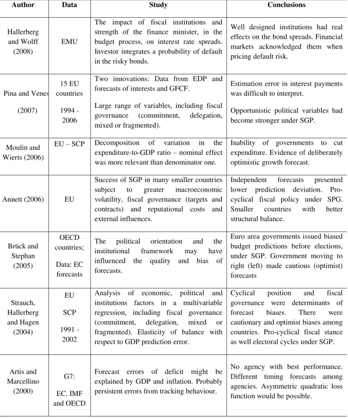
Table I. Related literature

Author Data Study Conclusions

Hallerberg and Wolff (2008)

EMU

The impact of fiscal institutions and strength of the finance minister, in the budget process, on interest rate spreads. Investor integrates a probability of default in the risky bonds.

Well designed institutions had real effects on the bond spreads. Financial markets acknowledged them when pricing default risk.

Pina and Venes

(2007)

15 EU countries

1994 - 2006

Two innovations: Data from EDP and forecasts of interests and GFCF.

Large range of variables, including fiscal governance (commitment, delegation, mixed or fragmented).

Estimation error in interest payments was difficult to interpret.

Opportunistic political variables had become stronger under SGP.

Moulin and Wierts (2006)

EU – SCP Decomposition of variation in the expenditure-to-GDP ratio – nominal effect was more relevant than denominator one.

Inability of governments to cut expenditure. Evidence of deliberately optimistic growth forecast.

Annett (2006) EU

Success of SGP in many smaller countries subject to greater macroeconomic volatility, fiscal governance (targets and contracts) and reputational costs and external influences.

Independent forecasts presented lower prediction deviation. Pro-cyclical fiscal policy under SPG. Smaller countries with better structural balance. Brück and Stephan (2005) OECD countries; Data: EC forecasts

The political orientation and the institutional framework may have influenced the quality and bias of forecasts.

Euro area governments issued biased budget predictions before elections, under SGP. Government moving to right (left) made cautious (optimist) forecasts Strauch, Hallerberg and Hagen (2004) EU SCP 1991 - 2002

Analysis of economic, political and institutions factors in a multivariable regression, including fiscal governance (commitment, delegation, mixed or fragmented). Elasticity of balance with respect to GDP prediction error.

Cyclical position and fiscal governance were determinants of forecast biases. There were cautionary and optimist biases among countries. Pro-cyclical fiscal stance as well electoral cycles under SGP.

Artis and Marcellino (2000) G7: EC, IMF and OECD

Forecast errors of deficit might be explained by GDP and inflation. Probably persistent errors from tracking behaviour.

No agency with best performance. Different timing forecasts among agencies. Asymmetric quadratic loss function would be possible.

3 Methodology

(12)

11

years and a range of economic predictable variables as large as possible. In this context deviation is defined by the realisation, r, minus the forecast, f:

, , i t ,

i t fi t

e r  _,(7)

where i denotes country and t is the period of prediction.

3.1 Forecasts from the European Commission

We will assess whether the deviation of the budget balance-to-GDP ratio can be explained by deviations of other economic variables. We will use two different approaches – unbalanced panels that will study a set of countries as well as seemingly unrelated regressions (SUR) in order to analyse each country in a particular way.

In addition, the study will also assess the deviations about the decomposition of the government budget constraint - snow ball effect of public debt stock, interest effect, nominal GDP effect, primary balance and other adjustments. This specification integrates not only adjustments with direct impact on government debt but also variables connected to the budget deficit. Therefore, the growth forecast accuracy would have an important role on taxes, expenditures and on the denominator of the ratio. The government budget constraint in (8) illustrates such dynamics:

1 ₁t t 1

t t t t t t

t

i n

g sf

b b b

n 



 _  _   



(8)

where b is the debt-to-GDP ratio, i is the implicit interest rate paid on the outstanding stock of

government debt, n is the nominal growth rate of the economy, g is the primary

spending-to-GDP ratio,  is the revenue-to-GDP ratio, and sf is the stock-flow adjustment-to-GDP ratio.1

Furthermore, the decomposition presented by Moulin and Wierts (2006) identifies the nominal and the denominator effects, which allows knowing whether the budget balance forecast error is coming from divergence predictions on GDP as well as from expenditure or revenue items. The decomposition of these effects can be done via

t n t t n t t t n t t n t t n t n t

G G G G G Y Y

Y Y Y Y Y

 _   _     _  

       

 _   _   _  

      _.(

9)

1_{The stock-flow adjustment includes differences in cash and accrual accounting, accumulation of financial}

(13)

12

Strauch, Hallerberg and von Hagen (2004) studied the elasticity of the budget balance with respect to the GDP prediction error , concluding that when actual output growth exceeds forecasts, the budget balance improves by 0.59 percentage points when compared with the budgetary prediction

0.07 0.59

balance growth

e   e v _.(10)

In this study we will take into account deviations not only of the budget balance-to-GDP ratio and of real GDP but also of the unemployment rate, investment and other variables.

3.2 Forecasts from the Portuguese Government

The Portuguese data will be studied with a particular detail, i.e. the deviation between forecasts of budget balance-to-GDP ratios and the respective realisations will be explained by divergence of predictions of real GDP growth and price variations. Furthermore, it will be possible to have the decomposition of the deviation of budget balance-to-GDP ratios between denominator and nominal effect, as well as identifying the size of temporary measures in recent years.

4 Empirical analysis

4.1 Data

The data base covers the vintage forecasts of the European Commission regarding the two publications per year – Spring and Autumn, while the Portuguese Government predictions come from the state budget reports and/or from other connected documents in a supplementary way detailed below.2 Predictions about real GDP, prices variation and balance are the main variables taken into account by these two last institutions. Therefore, some variables may be hidden, which would be an additional source of problems in the econometric analysis. Furthermore, Stability (or Convergence) Growth Programmes could have been an alternative data source because they include a set of variables required by the European institutions in order to present comparable information. However, this kind of analysis has been already used by other studies.

2

(14)

13

4.1.1 European Commission

There are two data bases about forecasts with different range of variables and periods. A data set3 for the period (1969-2011) includes the European Union, the Euro Area and the 15 oldest Member States4 since the year of adhesion to the EU. This dataset contains current year projections from the Spring publication, one year ahead projections from the Autumn

forecast, as well as realisations based on the “first available estimates” published in the

following year – the Spring estimates and values available in the Autumn, for the current year and year ahead, respectively. Some economic variables with available deviations are budget balance-to-GDP ratio, inflation, investment, unemployment rate, current account as percentage of GDP and employment variation.

Another data set was built for the EMU period (1999-2011) with twice a year vintage forecasts since Spring 1998 (original time span is 1998:1-2010:2) for the same set of countries, including a larger range of variables – real GDP, inflation, GDP deflator, unemployment rate, investment, general government gross debt, primary balance, revenue-to-GDP, expenditure-to-revenue-to-GDP, and budget balance-to-GDP ratios. Some variables were not available in the beginning of this period for all countries and Luxembourg had not available data in some indicators until later - Autumn 1999. This data base will allow econometric estimations as well as the decomposition of effects underlying the government budget constraint and revenue/expenditure-to-GDP ratios. It is important to stress that this data set includes realisations based on final results from AMECO and Eurostat.5 There are differences between data sets because the realizations for the period 1969-2011 are based on first estimates, while the outcomes for 1998-2011 contains revised data (and revisions usually contain systematic bias in Europe, see Castro, 2012).

Furthermore, the fiscal rules index published by the European Commission for the period 1990-2010 also will be taken into account, as a possible determinant of forecast deviations. This time span is longer when compared with existing studies about this subject, but it is not

3_{This data base was kindly provided by the DGECFIN and had been used in a previous study for the period}

1969-2005 (Melander, Sismanidis, & Grenouillea, 2007). Data base was updated until 2011 in line with authors criteria, notably realization based on the “first available estimates” instead of final results, which would have

revised values in some cases.

4_{Countries included are: Belgium; Germany; Greece; Spain; France; Ireland; Italy; Luxembourg; Netherlands;}

Austria; Portugal; Finland; Denmark; Sweden; United Kingdom.

(15)

14

as long as the data base (1969-2011) available for other variables, which then constrains a panel econometric estimation.

4.1.2 Portuguese Government 1977-2011

The set of available variables includes deviations of the budget balance-to-GDP ratio, real GDP growth rates and prices variation. The information comes from the state budget reports for recent years as well as from the State Budget Law, Decree-Law and Grandes Opções do Plano for the earlier period. The predictions underlying to the State Budget are available

during the end of previous year6. However, the State Budget Laws were available during the implementation year in case of elections, appointments of new a government or other political factors. The data set was then constructed covering each predictable variable with particular detail – source, universe, and publication date.7

The availability of information during 1970s and 1980s is scarce and the month of publication was different among years. For example, the prediction for 1979 was found in Previsões Macroeconómicas of October 1979 - real GDP and prices. In addition, projections for 1983

were another difficult case, and we used Grandes Opções do Plano for the medium term

published in 1981, for forecasts about real GDP and prices variation because predictions of economic variables were not available in 1983.

The prediction of the budget balance-to-GDP ratio of the Administrative Public Sector on accrual basis was the desirable variable connected with the budgetary forecasts during the 1970s, 1980s and 1990s, however, in some years there was only information on cash basis. The general government balance on accrual basis is the measure of public sector in recent years, which has been used by Eurostat.

The desirable measure of price variation is the GDP deflator. Still, it was not possible to find information about this variable for 1989 and 1990. Therefore, it was used a measure of inflation in a supplementary way – the variation of private consumption deflator and consumer prices index for 1989 and 1990 respectively.

The final data for the Portuguese case come from the National Accounts provided by the Statistics Portugal (INE) according to the European System Account as well as from the

6_{Actually, the government must present a draft of the State Budget and a deliver it to the Parliament until 15}

October, unless elections take place and a new government takes in this period.

(16)

15

Eurostat and AMECO data base. This information, reported by INE to European Institutions, is comparable with data from other member states.

4.2 Results

4.2.1 European Commission

4.2.1.1Analysis for 1969-2011

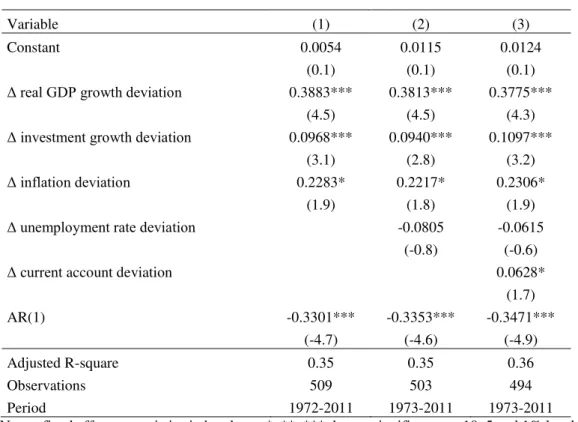
The estimations based on one year ahead forecasts (data from Autumn) suggests that the deviations of budget balance-to-GDP ratios may be explained by errors of projections about other variables – mostly real GDP growth, investment variation and inflation (see Table II). In regression (1), we may conclude that a favourable deviation of real GDP of 1 percentage point (pp) has a positive impact of 0.39 pp on the deviations of general government budget balance ratio. Higher inflation than predicted of 1pp may improve the balance-to-GDP ratio in 0.23pp. These effects may be associated with deviation of nominal GDP, in which higher growth means lower unemployment, less social benefits and higher tax receipts in line with expected with automatic stabilizers. Investment variations seem to present statistical significance, but the coefficient has a low magnitude.

The dependent variable and explanatory variables included in regressions are the following:

*

* *

( ₁ ₁) ₀ ( ) ₂ ( ₁ ₁)

1 1 1

* *

*

( ₁ ₁) ( ) ( ) ,

3

inf

4 1 1 5 1 1 6

(1)

t t _t _t t t

t t t t t t

gdp

b

inv

AR

un

cur



 _  _      _  _ 

 

 _  _   _  _   _  _ 



(11)

where ₍ * ₎

1 1

t t

b b

 _  _ denotes dependent variable (first difference of the budget balance ratio

(17)

16

Table II. Estimation for the first difference of the budget balance-to-GDP ratio

deviation, 1969-2011, ₍ * ₎

1 1

t t

b b

 _  _

Variable (1) (2) (3)

Constant 0.0054 0.0115 0.0124

(0.1) (0.1) (0.1)

Δ real GDP growth deviation 0.3883*** 0.3813*** 0.3775***

(4.5) (4.5) (4.3)

Δ investment growth deviation 0.0968*** 0.0940*** 0.1097***

(3.1) (2.8) (3.2)

Δ inflation deviation 0.2283* 0.2217* 0.2306*

(1.9) (1.8) (1.9)

Δ unemployment rate deviation -0.0805 -0.0615 (-0.8) (-0.6)

Δ current account deviation 0.0628* (1.7)

AR(1) -0.3301*** -0.3353*** -0.3471***

(-4.7) (-4.6) (-4.9)

Adjusted R-square 0.35 0.35 0.36

Observations 509 503 494

Period 1972-2011 1973-2011 1973-2011

Notes: fixed effects. t-statistics in brackets. *, **, *** denote significance at 10, 5 and 1% levels.

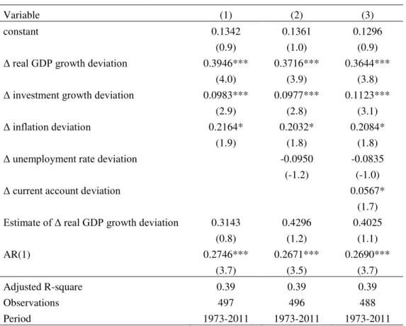
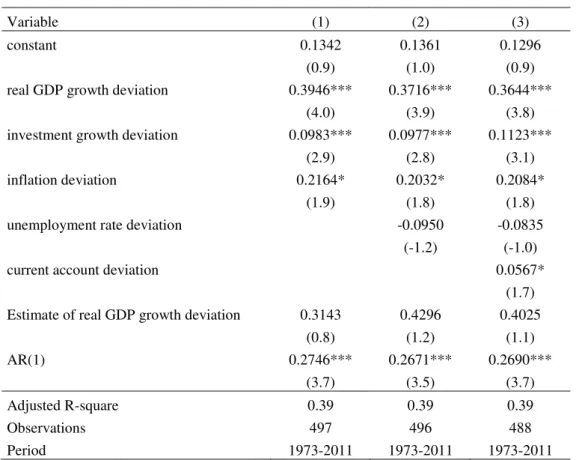
We analyzed endogeneity between dependent variable and real GDP growth deviation through instrument variables (IV) and two stage least squares (2SLS). The instruments were the lagged real GDP growth deviation (first and second lags). It was not found evidence of endogeneity. See Table III and Table A2.

The regressions take into account the estimate of real GDP growth deviation in order to evaluate its statistical significance

*

* * *

( ₁ ₁) ₀ ( ) ₂ ( ₁ ₁) ₃ ( ₁ ₁)

1 1 1

* * *

( ) ( ) ,

4 1 1 5 1 1 6 ₁ ₁ 7

^

inf

(1)

(

)

t t

t t _t _t t t

t t t t _t _t

gdp

b

inv

AR

gdp

un

cur



 _  _   _  _   _  _   _  _   _  _   _  _     





(12)

where

* *

* ₍ ₎ ₍ _),

0 1 1 1

1 1

^

(

gdp

_t

gdp

_t

)



gdp gdp

_t _t



gdp

_t

gdp

_t

      

 





 (13)

(18)

17

Table III. Estimation for the first difference of the budget balance-to-GDP ratio

deviation, 1969-2011, ₍ * ₎

1 1

t t

b b

 _  _ (instrumental variables)

constant 0.1342 0.1361 0.1296

(0.9) (1.0) (0.9)

Δ real GDP growth deviation 0.3946*** 0.3716*** 0.3644***

(4.0) (3.9) (3.8)

Δ investment growth deviation 0.0983*** 0.0977*** 0.1123***

(2.9) (2.8) (3.1)

Δ inflation deviation 0.2164* 0.2032* 0.2084*

(1.9) (1.8) (1.8)

Δ unemployment rate deviation -0.0950 -0.0835 (-1.2) (-1.0)

Δ current account deviation 0.0567* (1.7)

Estimate of Δ real GDP growth deviation 0.3143 0.4296 0.4025

(0.8) (1.2) (1.1)

AR(1) 0.2746*** 0.2671*** 0.2690***

(3.7) (3.5) (3.7)

Period 1973-2011 1973-2011 1973-2011

Notes: t-statistics in brackets. *, **, *** denote significance at 10, 5 and 1% levels

In this case, it does not seem that there is evidence of endogeneity because the estimated parameter for real GDP growth deviation does not present statistical significance.

Regression (2) shows that forecast deviations about the unemployment rate do not contribute to explain the dependent variable. On the other hand, in regression (3) we see that positive forecast errors in current account-to-GDP ratios have a positive and statistically significant effect on the budget balance deviation errors. Forecast errors of inflation, the unemployment rate and real GDP growth remain rather similar in magnitude in regressions (2) and (3). The average of real GDP deviations in the sample as a whole reveals a negative deviation, while inflation presents a positive one, which means the EC forecasts may have overestimated real growth and underestimated inflation, attaining eventually a similar nominal GDP with a different decomposition.

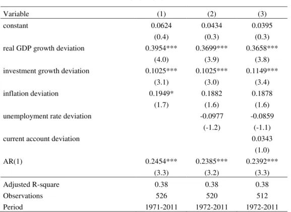
We used a first differences method in order to avoid eventual problems connected with

(19)

18

been taken into account as dummy variables such as in some studies. However, our panel data set (vintage forecasts) starts in the beginning of the 1970s, in which case there was a lack of information about fiscal rules. Therefore, one possible solution to overcome that likely problem may be a regression based on the first differences method.

Furthermore, given that the Durbin Watson statistics seems to reveal serial correlation when it was used deviation of predictions. Therefore, it was taken into account a AR(1) variable in order to address that issue. However, we have estimated the budget balance ratio deviation with fixed effects:

*

* * *

( ₁ ₁) ₀ ( ) ₂( ₁ ₁) ₃( ₁ ₁)

1 1 1

* *

( ) ( )

4 1 1 5 1 1 6

inf

(1)

t t

t t _t _t t t

t t t t

gdp

b

inv

AR

un

cur



      _  _               



.(14)

Table IV. Estimation for the budget balance-to-GDP ratio deviation, 1969-2011,

* (_b_t_₁_b_t_₁)

constant 0.0624 0.0434 0.0395

(0.4) (0.3) (0.3)

real GDP growth deviation 0.3954*** 0.3699*** 0.3658***

(4.0) (3.9) (3.8)

investment growth deviation 0.1025*** 0.1025*** 0.1149***

(3.1) (3.0) (3.4)

inflation deviation 0.1949* 0.1882 0.1878

(1.7) (1.6) (1.6)

unemployment rate deviation -0.0977 -0.0859

(-1.2) (-1.1)

current account deviation 0.0343

(1.0)

AR(1) 0.2454*** 0.2385*** 0.2392***

(3.3) (3.2) (3.3)

Period 1971-2011 1972-2011 1972-2011

Notes: fixed effects. t-statistics in brackets. *, **, *** denote significance at 10, 5 and 1% levels

(20)

19

Table V. Estimation for the budget balance-to-GDP ratio deviation, 1969-2011,

*

(_b_t_₁_b_t_₁) (instrumental variables)

constant 0.1342 0.1361 0.1296

(0.9) (1.0) (0.9)

(4.0) (3.9) (3.8)

investment growth deviation 0.0983*** 0.0977*** 0.1123***

(2.9) (2.8) (3.1)

inflation deviation 0.2164* 0.2032* 0.2084*

(1.9) (1.8) (1.8)

(-1.2) (-1.0)

current account deviation 0.0567*

(1.7) Estimate of real GDP growth deviation 0.3143 0.4296 0.4025

(0.8) (1.2) (1.1)

AR(1) 0.2746*** 0.2671*** 0.2690***

(3.7) (3.5) (3.7)

Period 1973-2011 1973-2011 1973-2011

Notes: fixed effects t-statistics in brackets. *, **, *** denote significance at 10, 5 and 1% levels

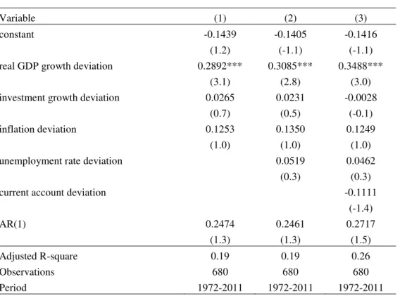
We also analyzed the estimations about the predictions of current year (prediction of t in year t), but results seemed statistically poor, which may be a signal that there is no systematic error in the estimated specifications in the short term. The real GDP growth deviation remains important (Table VI illustrates such evidence).

(21)

20

Table VI. Estimation for the budget balance-to-GDP ratio deviation, 1969-2011,

* (_b_t_b_t)

constant -0.1439 -0.1405 -0.1416

(1.2) (-1.1) (-1.1)

(3.1) (2.8) (3.0)

investment growth deviation 0.0265 0.0231 -0.0028

(0.7) (0.5) (-0.1)

inflation deviation 0.1253 0.1350 0.1249

(1.0) (1.0) (1.0)

unemployment rate deviation 0.0519 0.0462

(0.3) (0.3)

current account deviation -0.1111

(-1.4)

AR(1) 0.2474 0.2461 0.2717

(1.3) (1.3) (1.5)

Period 1972-2011 1972-2011 1972-2011

Notes: fixed effects. t-statistics in brackets. *, **, *** denote significance at 10, 5 and 1% levels

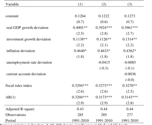
Another possibility is the inclusion of a fiscal rules index in order to proxy the quality of fiscal governance. Our unbalanced panel covers now a shorter period, 1990-2010, because the fiscal rules index, which is connected with fiscal governance and may be a measure of budgetary process, has a smaller time span availability. This fiscal rule index is derived from a questionnaire8 that has been sent to all EU member states, which integrates a large range of questions. The survey includes information about nature of the fiscal rule, covered subsectors, legal base of the rule, monitoring of compliance, enforcement of compliance, media and public reaction in case of non-compliance and long-term impact.

Table VII presents estimation results with the fiscal rule index, and we see that the precious results are kept. Moreover, in regression (1) a favourable deviation of 1 pp in real GDP means a positive deviation of 0.40 pp in the error of the general government budget balance ratio. In addition, deviation errors in inflation of 1 pp result in an impact of 0.46 pp on the dependent variable, while an error of investment variation imply a 0.11 pp effect.

(22)

21

The fiscal rule index is statistically significant, as expected due to previous studies. In fact, we can conclude that the predictions of the EC about a country with a better fiscal rule index tends to increase more likely a favourable (positive) deviation (or reduce an unfavourable one) in the error forecast of the budget balance ratio.

Table VII. Estimation of budget balance-to-GDP ratio deviation, 1990-2010, ₍ * ₎

1 1

t t

b  b 

constant 0.1264 0.1222 0.1273

(0.7) (0.6) (0.7)

real GDP growth deviation 0.4001** 0.3924*** 0.3961***

(2.5) (2.8) (2.7)

investment growth deviation 0.1138** 0.1126** 0.1314**

(2.2) (2.1) (2.2)

(1.8) (1.8) (1.8)

(-0.3) (-0.1)

(-0.0)

fiscal rules index 0.3294*** 0.3273*** 0.3270**

(2.6) (2.6) (2.5)

AR(1) 0.3204*** 0.3173*** 0.3143***

(2.9) (2.9) (2.8)

Period 1991-2010 1991-2010 1991-2010

Notes: t-statistics in brackets. *, **, *** denote significance at 10, 5 and 1% levels

(23)

22

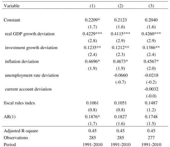
Table VIII. Estimation of budget balance-to-GDP ratio deviation, 1990-2010,

* (_b_t_₁_b_t_₁)

Constant 0.2209* 0.2123 0.2040

(1.7) (1.6) (1.6)

(2.8) (2.9) (2.9)

investment growth deviation 0.1235** 0.1212** 0.1386**

(2.4) (2.3) (2.4)

(1.9) (1.9) (2.0)

(-0.7) (-0.2)

(-0.0)

fiscal rules index 0.1061 0.1051 0.1487

(0.8) (0.8) (1.2)

AR(1) 0.1876* 0.1827 0.1748

(1.7) (1.6) (1.5)

Period 1991-2010 1991-2010 1991-2010

The regressions in Table VIII does not include data before 1990 of countries that entered in the EU before that year due to the unavailability of fiscal rules index as mentioned before. Furthermore, there is no available information about 2011.

Returning to the longer data set (1969-2011), we can estimate a seemingly unrelated regression (SUR), i.e. estimating regressions with the same variables for each individual country. However, the size of sample is different among countries because the availability of variables for each country is connected with the year they entered the in EU. Therefore, the oldest Member States – France, Italy, Germany, the Netherlands, Belgium and Luxembourg –

have 41 annual observations, while Finland, Sweden and Austria have 17 observations.

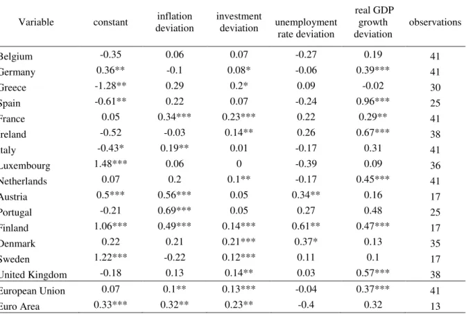
In Table IX, the SUR estimation results of t+1, in year t, reveal that variables have different

(24)

23

For example, in the case of the EU with 41 observations there are three variables with statistical significance – inflation (0.10 pp), investment (0.13 pp) and real GDP (0.37 pp). In case of France, the same set of variables present statistical importance, but with different scale of parameters, 0.34 pp, 0.23 pp and 0.29 pp, respectively. The general specification for country i is presented below:

* * *

( _1, _1,) _0, ( _1, _1,) _2,( _1, _1,)

1,

* *

( ) ( )

3, 1, 1, 5, 1, 1,

inf

i t i t i

t i t i _i i t i t i

i t i t i i t i t i

b

inv

gdp

un



  _  _              



. (15)

Table IX. Estimation of balance-to-GDP ratio deviation, SUR, 1969-2011,( )

Variable constant _deviationinflation investment _deviation unemployment rate deviation

real GDP growth

deviation observations

Belgium -0.35 0.06 0.07 -0.27 0.19 41

Germany 0.36** -0.1 0.08* -0.06 0.39*** 41

Greece -1.28** 0.29 0.2* 0.09 -0.02 30

Spain -0.61** 0.22 0.07 -0.24 0.96*** 25

France 0.05 0.34*** 0.23*** 0.22 0.29** 41

Ireland -0.52 -0.03 0.14** 0.26 0.67*** 38

Italy -0.43* 0.19** 0.01 -0.17 0.31 41

Luxembourg 1.48*** 0.06 0 -0.39 0.09 36

Netherlands 0.07 0.2 0.1** -0.17 0.45*** 41

Austria 0.5*** 0.56*** 0.05 0.34** 0.16 17

Portugal -0.21 0.69*** 0.05 0.27 0.48 25

Finland 1.06*** 0.49*** 0.14*** 0.61** 0.47*** 17

Denmark 0.22 0.21 0.21*** 0.37* 0.13 35

Sweden 1.22*** -0.22 0.12*** 0.11 0.1 17

United Kingdom -0.18 0.13 0.14** 0.03 0.57*** 38

European Union 0.07 0.1** 0.13*** -0.04 0.37*** 41

Euro Area 0.33*** 0.32** 0.23** -0.4 0.32 13

Note: Total system (unbalanced), 537 observations. Linear estimation after one-step weighting matrix. t-statistics in brackets. *, **, *** denote significance at 10, 5 and 1% levels.

4.2.1.2 Analysis for 1999-2011

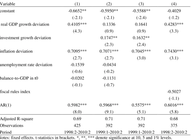
In a panel approach for the period 1998:1-2010:2 the deviation of forecasts of general government budget balance ratio in the year t+1 may be explained by other economic variables projected to t+1, notably divergences in inflation and in real GDP, see estimation results in Table X. Furthermore, deviations of observed budget balances in the previous year t

(25)

24

the unemployment rate as well as the period when forecasts were published (Spring or Autumn) does not present statistical significance. There is no evidence of endogeneity (See appendix Table A3).

Regression (1) of Table X suggests that there is a favourable deviation of 0.67 pp of budget balance-to-GDP ratios in case of no deviations about other variables. Errors in inflation forecasts (1 pp) imply an upward deviation of 0.71 pp and real GDP positive growth deviations of 1 pp cause an upward realization of 0.41 pp in the budget balance ratios’ error

deviations. The estimation results in regression (1) are then rather consistent with the automatic stabilizers mechanisms and an imperfect indexation tax system. Deviations in total investment growth regressions (2) and (3) have a statistical significance, which may imply that higher than expected investment realizations may also be connected with higher real GDP.

Table X. Estimation of balance-to-GDP ratio deviation, 1998:1-2010:2, ₍ * ₎

1 1

t t

b  b 

Variable (1) (2) (3) (4)

constant -0.6652** -0.5950** -0.5588** -0.4029

(-2.1) (-2.1) (-2.4) (-1.2)

real GDP growth deviation 0.4105*** 0.1336 0.1641 0.4283***

(4.3) (0.9) (0.9) (3.3)

investment growth deviation 0.1747** 0.1632**

(2.3) (2.4)

inflation deviation 0.7095*** 0.7071*** 0.7045*** 0.7430***

(2.7) (2.7) (3.0) (3.1)

(-0.6) (-0.2)

balance-to-GDP in t0 -0.0202 -0.1131

(-0.1) (-0.7)

fiscal rules index -0.5027

(-1.1)

AR(1) 0.5982*** 0.5968*** 0.5575*** 0.6016***

(8.0) (9.1) (5.1) (5.8)

Adjusted R-square 0.69 0.71 0.71 0.68

Observations 425 392 392 375

Period 1998:2-2010:2 1999:1-2010:2 1999:1-2010:2 1998:2-2010:2

(26)

25

Commission forecasts are more able to take into account the different performance of fiscal governance among countries in the EMU period. Some previous studies (von Hagen, 2010) have reported the importance of that kind of determinants. Therefore, fiscal governance indicators would have statistical importance in the case of data provided by the national governments such as Stability (or Convergence) and Growth Programmes. The fiscal rules for the budget balance ratio based on the output gap would have been wrong, because potential output bias has been relevant. Therefore, the admissible deficit in real time would have exceeded final values (Kempkes, 2012).

Interestingly, Martins (2012) concludes that the European Commission forecasts were biased, which may be problematical when used as benchmark to evaluate the quality of government forecasts. However, in some cases such as Portugal and Italy, with optimistic government predictions of growth and public accounts, the European Commission forecasts may be a useful reference.

In addition, we also assessed the determinants of the forecasts deviations of gross debt of the general government. However, the results show that some variables (budget balance ratio deviation and real GDP growth error) present strong statistical significance.

The dependent variable ₍ * ₎ 1 1

t t

debt  debt  is the deviation of the prediction for general

government debt:

*

* * *

( ₁ ₁) ₀ ₁ ₁ ₁ ( ) ₃( ₁ ₁)

1 1

2

* *

*

( ₁ ₁) ( ) ( )

4 5 1 1 6 7 8

(

)

(1)

inf

t t t t t t t t

fiscalrules

t t t t t t

gdp

debt

b

inv

AR

un

b b



 



     

       

      

   







(27)

26

Table XI. Estimation of debt-to-GDP ratio deviation, 1998:1-2010:2,

* ( ₁ ₁)

t t

debt  debt 

Variable (1) (2) (3) (4)

Constant 1.2943* 1.1611 1.1133 0.7012

(1.7) (1.4) (1.4) (0.8)

balance-to-GDP in t+1 -0.5933*** -0.5849*** -0.6400*** -0.6178***

(-5.6) (-4.5) (-6.4) (-5.9)

real GDP growth deviation -0.8654*** -0.8380*** -0.8729*** -0.8531***

(-4.5) (-3.2) (-5.1) (-4.9)

investment growth deviation -0.0113

(-0.1)

inflation deviation -0.2409 -0.3420

(-0.7) (-0.8)

unemployment rate deviation 0.5722* 0.5880* 0.6070* 0.6181*

(1.9) (1.9) (1.9) (1.9)

balance-to-GDP in t0 -0.9954*** -0.9749*** -1.0050*** -1.0067***

(-15.7) (-13.1) (-15.8) (-15.4)

fiscal rules index 0.7610*

(1.7)

AR(1) 0.7699*** 0.7819*** 0.7690*** 0.7654***

(14.3) (14.9) (13.8) (13.6)

Adjusted R-square 0.85 0.85 0.85 0.84

Observations 425 292 425 375

Period 1998:2-2010:2 1999:1-2010:2 1998:2-2010:2 1998:-2010:2

Turning now to the seemingly unrelated regression approach it would be desirable conclude that deviations in variables of some countries could explain divergence of balance relative to GDP. The serial correlation is an additional problem when estimating the regressions. The specification is the following one:

*

* *

( _1, _1,) _0, ( ) _2,( _1, _1,)

1, 1,

1,

* *

( ) ( ) _6,

3, 1, 1, 5, 1, 1,

inf

(1)

i t i t i

t i t i _i _t _i _t _i i

i

i t i t i i t i t i

gdp

b

AR

un

in

(28)

27

Table XII. Estimation of balance-to-GDP ratio deviation, 1999:1-2010:2₍ * ₎ 1, 1,

t i t i

b  b 

Variable constant

real GDP growth deviation

inflation

deviation unemployment rate deviation

investment

deviation AR(1) Observations

Belgium -0.3 0.75*** 0.48*** -0.34** -0.06 0.42*** 23

Germany 0.53** -0.21 0.44** -0.3*** 0.3*** 0.45*** 23

Greece -4.65*** 0.4* 1.47*** 0.94*** 0.07 0.59*** 23

Spain -0.42** 1.28*** -0.06 0.09 0.26*** 0.09 23

France -0.16 0.6*** 0.57*** -0.07 -0.01 0.44*** 23

Ireland -0.79 0 1.1*** 1.51*** 0.56*** 0.15 23

Italy -0.48 0.37* 0.24 -0.77*** -0.06 0.62*** 23

Luxembourg 1.01 -0.07 0.53*** -0.56** 0.17*** 0.62*** 23

Netherlands -0.02 0.53*** -0.04 -0.63** 0.31*** 0.67*** 23

Austria -0.45 -0.05 0.75** -0.53* 0.12 0.43*** 23

Portugal -1.58** 0.4 1.42*** -0.08 -0.12 0.59*** 23

Finland 0.06 0.39*** 0.37** -1.15*** -0.05 0.72*** 23

Denmark 1.61** 0.51*** 0.62*** -0.61** -0.01 0.72*** 23

Sweden 0.33 -0.15 -0.25 -0.46*** 0.25*** 0.66*** 23

United Kingdom -1.33** 0.76*** 1.45*** 0 0.14** 0.74*** 23

European Union -0.29 0.75*** 0.55*** -0.37** -0.1 0.49*** 24

Euro Area -0.05 0.19 0.45*** -0.2 0.19*** 0.44*** 23

Note: Total system (unbalanced), 392 observations. Linear estimation after one-step weighting matrix. t-statistics in brackets. *, **, *** denote significance at 10, 5 and 1% levels.

We used a AR(1) parameter in order to overtake serial correlation, however, this problem remain about half of the cases. For example, in Spain there are three variables with statistical significance – constant (-0.42 pp), real GDP growth deviation (1.28 pp) and total investment (0.26 pp), while in Ireland there are three other variables – inflation error (1.1 pp), unemployment rate (1.51 pp) and total investment (0.56 pp).

4.2.1.3 Government Budget constraint 1999-2011

(29)

28

effect, primary balance effect, and stock flow adjustments because some predictable variables were not available in some years for all countries.9 Again, the period under analysis covers semi-annual vintage forecasts from Autumn 1999 to Autumn 2010.

Table XIII presents the medium deviation (ME = realization - forecast) for the 15 Member States, the European Union and the Euro zone. 10 Predictions were published in year t for year t+1, including both Spring and Autumn forecasts. The European Commission has predicted on average positive (negative) variations of gross debt of general government with respect to GDP in some (other) countries, however, realizations have been higher (less negative or positive) than forecasted, i.e. we may conclude that there may have been a bias – optimistic predictions. Figure 1 also illustrates those results.

Table XIII. Government Budget Constraint (medium deviations - percentage points of GDP)

Country ∆ Debt t+1

interest effect t+1

nominal effect t+1

snow ball effect t+1

Primary Balance t+1

Stock flow t+1

Belgium 1.10 -0.23 0.27 0.04 0.50 0.55

Germany 1.46 -0.06 0.37 0.31 0.11 1.04

Greece 6.19 0.29 1.67 1.96 4.48 -0.25

Spain 0.56 -0.12 -0.05 -0.17 1.29 -0.56

France 1.33 -0.12 0.26 0.14 0.76 0.43

Ireland 4.48 0.06 0.99 1.04 2.79 0.65

Italy 1.72 0.02 1.12 1.14 0.66 -0.09

Luxembourg 0.90 0.02 -0.02 0.00 -1.52 2.43

Netherlands 1.17 -0.21 0.28 0.07 0.67 0.43

Austria 0.66 -0.11 -0.05 -0.16 0.51 0.31

Portugal 3.41 -0.03 0.73 0.71 1.74 0.97

Finland 0.96 -0.22 0.21 -0.01 -0.11 1.08

Denmark 1.26 -0.28 0.17 -0.11 0.10 1.27

Sweden 0.60 -0.55 0.24 -0.30 0.60 0.30

United Kingdom 2.21 0.09 0.22 0.31 1.04 0.86

European Union 1.40 -0.07 0.58 0.51 0.76 0.13

Euro Area 1.40 -0.05 0.44 0.39 0.72 0.30

Results show that the European Commission has underestimated the positive variation of general government gross debt as percentage of GDP with a particular size in Greece, Ireland

9_{Data for Luxembourg had not all variables in Autumn 1999.}

(30)

29

and Portugal, especially in the primary balance. The deviation in the snow ball effect is negative or positive among countries, but close to zero (sees Table XIII).

Figure 1. Government Budget Constraint

(medium deviations - percentage points of GDP)

-2,0 -1,0 0,0 1,0 2,0 3,0 4,0 5,0 6,0 7,0

pp of GDP Government Budget Constraint (medium deviations - pp of GDP)

snow ball effect t+1 Primary Balance t+1 Stock flow t+1 ∆ Debt t+1

The European Commission forecasts would be unbiased in case of ME = 0 or close to zero, however, the track record seems to show an optimistic bias. This result in the budget government constraint may be explained a little by deviation in other economic variables –

nominal GDP growth and weight of interest payments as gross debt of general government (see Table XIII).

In the case of Ireland there was a particular situation of financial crisis since 2009, in which deficit of general government attained 14%, 31.2% and 13% in 2009, 2010 and 2011 respectively.

4.2.1.4 Expenditure-to-GDP ratio: numerator and denominator effects

(31)

30

Table XIV. Decomposition about deviation of expenditure-to-GDP ratio

Country Expenditure ratio _∆ t+1

numerator effect

denominator effect

Belgium 0.41 0.34 0.07

Germany 0.14 -0.26 0.40

Greece 0.94 0.70 0.25

Spain 0.32 0.49 -0.16

France 0.58 0.39 0.20

Ireland 2.15 1.44 0.71

Italy 0.52 0.11 0.41

Luxembourg 0.29 0.24 0.05

Netherlands 0.47 0.47 0.00

Austria 0.25 0.22 0.04

Portugal 0.72 0.55 0.18

Finland 0.67 0.28 0.40

Denmark 0.63 0.35 0.29

Sweden 0.00 -0.72 0.72

United Kingdom 0.66 -0.59 1.26

European Union 0.43 0.07 0.36

Euro Area 0.43 0.18 0.25

Since in most countries the average prediction was for negative variations of expenditure relative to GDP (with the exception of Luxembourg, the United Kingdom and Spain), we may conclude that realizations of variations have not been negative as forecasted.

Figure 2. Decomposition of expenditure-to-GDP deviation

-1,0 -0,5 0,0 0,5 1,0 1,5 2,0 2,5

pp of GDP Decomposition of expenditure-to-GDP deviation

(32)

31

The results also suggest that the European Commission projections have initially some optimistic bias about the spending-to-GDP ratio in most countries, which afterwards is not fulfilled. This outcome is rather in line with the results of Moulin and Wierts (2006), who studied the government forecast through the SGPs, showing the inability of governments to cut expenditure and reporting also evidence of deliberately optimistic growth forecasts in order to justify nominal spending increases.

The forecasts about decomposition of the nominal/numerator and the denominator effects were consistently, in the entire sample, i.e. a favourable path of nominal GDP and an in increase of nominal expenditure, in which the denominator effect was stronger than the nominal/numerator one in most countries.

The deviations in the nominal/numerator effect in Germany, Sweden and the United Kingdom have been favourable, which means that predictions about the variation of nominal expenditure were lower than realizations while in another countries increase of nominal expenditure became higher than predicted.

In addition, deviations of the denominator effect mean that GDP nominal growth presented a lower contribution to reduce the expenditure-to-GDP ratio than predicted in most countries (an exception was Spain). Furthermore, it would still be possible to study the decomposition of nominal GDP growth between real output variation and deflator increase as mentioned before.

4.2.1.5Revenue-to-GDP ratio: numerator and denominator effects

Again for the same period of EC vintage forecasts, from Spring 199911 to Autumn 2010, regarding predictions in year t to year t+1 as before, the decomposition of revenue ratios between nominal/numerator and denominator effects does not seem to present a pattern. Table XV presents the decomposition of the revenue ratio in the same way as the expenditure one, and we can see that the European Commission predictions seem to have overestimated the variation of the revenue ratios in most cases, except in Spain. The medium forecast of revenue ratio variation in this period was negative for most countries and positive in some cases (Portugal, Spain and the United Kingdom). Therefore, realizations have been as favourable as predicted.

(33)

32

Table XV. Decomposition about deviation of revenue-to-GDP ratio

Country Revenue ratio _∆ t+1

numerator effect

denominator effect

Belgium 0.31 0.25 0.06

Germany 0.18 -0.19 0.37

Greece 0.16 -0.24 0.40

Spain -0.40 -0.19 -0.21

France 0.13 -0.04 0.17

Ireland 0.38 -0.01 0.40

Italy 0.37 -0.02 0.39

Luxembourg 0.24 0.29 -0.05

Netherlands 0.09 0.12 -0.03

Austria 0.24 0.20 0.04

Portugal 0.47 0.27 0.20

Finland 0.73 0.40 0.34

Denmark 0.64 0.37 0.27

Sweden 0.12 -0.61 0.73

United Kingdom 0.02 -1.01 1.03

European Union 0.11 -0.21 0.32

Euro Area 0.14 -0.08 0.22

The forecasts about the decomposition of the numerator denominator effects show the same path in all countries, similarly to the case of expenditure ratios, specifically a positive path of nominal GDP and a raise of nominal revenue, in which the denominator effect would be stronger than the numerator effect in most countries (exceptions are Portugal, Spain and the United Kingdom as mentioned before).

(34)

33

Figure 3. Decomposition of revenue-to-GDP deviation

-1,2 -0,6 0,0 0,6 1,2

pp of GDP Decomposition of revenue-to-GDP deviation

numerator effect denominator effect Revenue ratio ∆ t+1

4.2.2 Portuguese Government forecasts

4.2.2.1Regression analysis

Notwithstanding some tests about serial correlation explained below, regression (1) in Table XVI shows that real GDP growth deviations are statistically significant at the 1% level. Therefore, a deviation of 1 pp between real GDP growth and the predicted real GDP has a positive impact of 0.64 pp on the deviation of the budget balance ratio. In line with automatic stabilizers, a higher real GDP growth may be connected, for instance, with a lower level of social benefits and increasing revenues from social security contributions as well as increases in tax revenues. In addition, price growth deviations have a similar effect, i.e. a difference of 1 pp between realization and prediction has a positive impact on the budget balance-to-GDP ratio of 0.48 pp. In this case the positive impact of the deviation may be connected with the imperfect tax indexation system of some taxes – especially direct ones, i.e. the taxation is defined in the State Budget in line with the prediction of nominal income. However, a higher level of income due to higher inflation would mean larger revenues for the government.