MCE - A MODEL FOR THE PORTUGUESE EXTERNAL TRADE ()

Estudos de Economia, vol. II, n.• 1, Set.·Dez .. 1981

MCE -

A MODEL FOR THE PORTUGUESE

EXTERNAL TRADE

(*)

M. Margarida Ponte Ferreira

Introduction.

1 - Structure and basic assumptions. 2 - The price submodel.

3 - The quantity submodel. 4 - Parameter values:

a) Coefficients in the price equations; b) Price elasticities lor exports and imports.

5 - Testing the model:

a) Estimates and observed values; b) Over and underestimation; c) Average prediction errors;

d) Errors related to the normal intensity of change of the variables.

6 -Concluding remarks. Appendix.

Introduction

In the course of 1979-1980 a model for external trade has been implemented for the Portuguese economy with Norwegian assistance. The discussion of the model's basic assumptions, as well as the collection of data to test the model, took place in March/April 1979, at The Central Planning Department (DCP) in Lisbon. From then to July the same year the model was programmed, .and, up to the spring 1980, work was carried out at the DCP to give the parameters empirically based values and to test the forecasting abilities of the model (1).

This paper is intended to describe the model and to present some comments on parameter values and model results, which were obtained at the DCP in testing different basic equations of the model.

1 - Structure and basic assumptions

The model for the Portuguese external trade, which has been named MCE (2_{), is based on the Norwegian model for competitiveness KONK (3).}

(*) Oslo, October 1980.

( 1) Most empirical work was carried out by Alzira Cabrita, a member of the DCP's

technical staff.

(2) From Modelo de Comercio Externo (model lor external trade).

The sectoral desaggregation and some of the basic assumptions have, however been changed, in order to adapt the model to the characteristics of the Portuguese economy. In particular, the number of sectors was extended from four to twelve and, for each sector exposed to foreign competition, a distinction was made between export and domestic prices (in KON K's 1978 version only output prices were used).

In external trade models it has been often assumed that exports and imports develope as a result of factors affecting the growth of markets and of factors affecting the market shares. Market shares are usually supposed to depend on the price (or other terms) competitive position and on the product mix of demand.

The MCE model, as well as KONK, only determines the changes in the

import shares and export market shares resulting from changes in the price

competitive position. Therefore, to forecast total exports and imports,

account has to be taken, outside the model, of the growth and composition of demand.

Although there is no formal relation with the macroeconomic

input-output model MODEP (4

) the MCE model may be used as a pre-model for

MODEP . since it endogenises variables which are exogenous in MODEP. These variables are: export and domestic prices for sectors exposed to foreign competition, import shares and export market shares (5_{). In order to} make it easier to use MCE in connection with MODEP, the sectors in MCE were defined as aggregates of MODEP sectors. The sectoral definition was made on the basis of the type of foreign competition the sectors are exposed to. Account was taken, for each sector, of the relative weight of the sector's production which could be affected by relative price competition. Therefore, exposed sectors for which a very low relative price elasticity was expected were classified as sheltered sectors. The following sector classification was considered:

a) Sectors competing abroad (export oriented):

1 - Fishing and fish conserves; 2 - Food;

3 - Beverages and tobacco; 4 - Textiles;

5 - Clothes and shoes; 6 -Wood, cork and furniture;

7 - Paper and pulp;

8 - Electric material;

9 - Ship building and reparing.

( 4 ) From Modelo para a Economia Portuguesa, a model built in Portugal in 1976·1977

with assistance of Norwegian experts. This model is an aggregated and simplified version of MODIS IV.

(5) In MODEP the exogenous variable is the volume of exports.

b) Sectors competing at home (import competing):

10 - Metalic products;

11 - Non-electric machines.

c) Sheltered sectors:

12-Others.

The model is formed by a price submodel and a quantity submodel.

The price submodel determines cost and price changes for all sectors. The

cost equations are based on an input-output table for the base year (assuming the cost structure to be constant over time). The price equations determine price changes as a function of cost changes and, for the exposed sectors, also as a function of «world market price» developments.

The quantity submodel determines the changes· in import and export

market shares as a function of the relative price competitive position. The relative price competitive position is defined by the difference between changes in export or domestic prices and changes in the corresponding «world market prices», for a certain period.

In MCE all cost, price and market share variables are defined as percentage changes from the year before.

2 - The price submodel

The basic assumption in the price submodel is that, in the sheltered sector, price changes are entirely cost determined, while in the exposed sectors prices are also influenced by international prices for similar products.

For all sectors, cost changes are given by:

(1) C;

=

(ai1 P/1

+ ...

r12 P/12

+

a;M ZMM;

+

a;L W;) . 0" 1

(i

=

1 . . . 12)

where the vector (a;1, ... , a;12. a;M, a;L} represents the base year cost structure for sector

i,

with:

a;1

=

value of deliveries from sector j to sector

i

per unit of gross

value of production in sector i;

a;M

=

value of imports to sector i per unit of gross value of production in sector

i;

a;L

=

wage costs per unit of gross value of production in sector i;

0;

=

~ a,i

+

a,M

+

a,L

=

current costs as a share of gross value

1

(2)

And:

C;

=

changes in sector i's current costs;

PI;

=

changes in sector i's domestic prices;

W;

=

changes in unit wage costs, defined by the changes in nominal wages WO; adjusted to changes in productivity Y;

(W;

=

WO;- Y;).

For the sheltered sector, prices are given by cost and profit changes:

Pl,2 = Bl,2 C,2

+

(1 -

Bid

G

where Bl,2 represents the percentage of costs in sector 12's gross value of production. To assume Bl,2 constant over time means all cost components developing at the same rate. G is the change in unit profits in sector 12. It may be obtained from:

(3) G

=

H

+

W,2

with H refering the percentage change (exogenous) of the ratio between profits and wages (6

) and W,2 is the change in unit wage costs in sector 12.

Whenever it is assumed a constant income distribution between labour and capital, variable G in equation 2) may be substituted by W,2 (profits and wages develope at the same rate).

For the sectors exposed to foreign competition (i

=

1 ... 11 }, the model distinguishes between export prices (PX;) and domestic prices (PI;),

with:

(4) PX;

=

BX; C;

+

(1 - BX;) ZX;

(i

=

1 ... 11)

ZX; is the change in world market prices for products corresponding to sector

i

(exogenous) (7

) and the coefficient BX; gives the proportion of cost

changes passed on export prices.

And:

(5) PI; 8/; C;

+

(1 - 8/;) ZM;

(i

=

1 ... 11)

(6) The percentage changes (H) of the ratio between profits and wages may be assumed on the basis of the values given by a trend line h

=

a + b(t), where h represents the trend values for that ratio:

H=~

h

with ZM i representing the change in import prices of products competing

with sector i's goods (exogenous) (B) and 81 i is the cost incidence coefficient

in domestic price changes (9 ).

Equations 1) to 5) determine domestic prices PI i . . . Pl12 and export prices PX 1 . . . PX 11 from the coefficients 8l1 .. : 81,_{2 ,} 8X _{1 . . .} 8X ₁₁ and from exogenous values for ZM1 . . . ZM11, ZX 1 . . . ZX 11 , W01 . . . W012 , Y1 . . . Y12 .

The model. may also determine the changes in the consumer price index PC and in real wages WRi:

(6)

with:

PC

=

~

v1

Pl1 j

~ Vj

=

1 I

where

v

₁ is the weight of each sector in the price index.

(7)

WRi

=

WCi- PC

(i

=

1 . . . 12)

Finally, sectoral prices Pi may be computed as weighted averages of

domestic prices PI i and export prices PXi using as weights the importance of the sector's production delivered to domestic and foreign markets:

8)

Pi

= ·;·

i PXi

+

(1 - ·: i) Pli

(i

=

1 ... 11)

with ·: ₁ representing the proportion of exports in .sector i's total production.

3 - The quantity submodel

In the quantity part of the model, changes in export market shares (1°) and in import shares (11

) are assumed to be determined by changes in the relative price competitive position. Changes in relative competitiv(;:lness

(B) See what was said about ZXi (foot note 7).

(9) It seems reasonable to assume domestic prices to be more influenced by cost developments than export prices and, therefore, 8/i would be higher than 8Xi. Obviously an economic policy oriented towards increased cost-price competitiveness does only make sense m the case of relatively high 8X and/or 8/.

( 10) Export market shares are defined as the ratio between the country's exports and the trading parteners· total imports.

abroad are gjven, in the model, by lagged changes in export prices compared with changes in international prices for similar commodities:

(9) QX;

=

~ lk (PX; - ZX;) t-k

k

(i

=

1 ... 11)

where I k are weights associated with the lag distribution.

Changes in export market shares are given by:

(10) MX;

=

SX; QX;

(i

=

1 ... 11)

where sx; is the price elasticity of export market shares in the above considered period.

For the domestic market, changes in the relative competitive position are given, in the model, by lagged changes in domestic prices compared with changes in import prices for similar goods:

(11) QM;

=

~ nk (PI; - ZM;) t·k

k

(i

=

1 ... 11)

nk being the lag structure.

Changes in import shares are then resulting from:

(12) MM;

=

sm; QM;

where sm; is the price elasticity of import shares in the period

t-k.

4 - Parameter values

Attempts were made to estimate the parameters of the model on OECD and on national data. Estimation was, however, based on a rather limited number of observations (1972-1976) (12_{) and results were clearly}

doubtful. It was, therefore, decided to take estimation results as simple indicators for the parameter values, i.e., to consider these estimates together with other information (knowledge on the sectors, economic literature) in setting those values.

are:

The parameters for which empirically based values have been used

Coefficients for cost incidence on export price relations (designated by BX);

Coefficients for cost incidence on home market prices (designated by 8/);

Elasticity of export market shares with respect to relative prices (designated by sx);

Elasticity of import shares with respect to relative prices

(designated by sm).

As the coefficients of the price equations (coefficients for costs and coefficients for world market prices) are assumed to sum one, the incidence of world market prices on export and domestic prices is given by the difference of the cost coefficients to the unity (respectively 1 - BX and

1 - 8/).

Table no. 1 shows the values set at DCP for the parameters in the price equations and table no. 2 the values for the price elasticities of exports and imports. These values do not correspond to estimation results, although they were set by taking estimates into consideration.

TABLE NO. 1

Coefficients in the price equations

Export prices Domestic prices Exposed sectors

BX; 1-BX; Bl; 1-8/;

1 - Fish and conserves . . . . .... 0.70 0.30 0.90 0.10

2 -Food ... 0.20 0.80 0.80 0.20

3 - Drinks and tobacco . . . . . .... 0.10 0.90 0.90 0.10

4 - Textiles ... 0.15 0.85 0.80 0.20

5 - Cloths and shoes . 0.40 0.60 0.98 0.02

6 - Wood, cork and furniture ... ... 0.90 0.10 0.50 0.50 7 - Paper and pulp . . . ... . ... 0.05 0.95 0.20 0.80

8 -Electric material . ... 0.10 0.90 0.90 0.10

9 - Ship building and reparing ... 0.60 0.40 0.98 0.02

10 - Metal products ... . . . 0.90 0.10 0.20 0.80

11 - Non-electric machines .. .... . ... 0.20 0.80 0.85 0.15

Where:

BX i - coefficient for cost incidence on export prices; 81 i - coefficient for cost incidence on domestic prices; 1 - 8X i -world market price incidence on export prices; 1 - 81 i -world market price incidence on domestic prices.

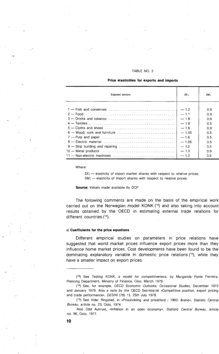
TABLE NO. 2

Price elasticities for exports and imports

Exposed sectors SXi

1 - Fish and conserves ... . -1.2 2 - Food ... . -1.1 3 - Drinks and tobacco ... . -1.8 4 -Textiles ... . -1.8 5 - Cloths and shoes ... . -1.8 6 - Wood, cork and furniture ... . -1.05 7 - Pulp and paper ... . -1.6 8 - Electric material ... . -1.05 9 -Ship building and reparing ... . -1.2 1 o - Metal products ... . -1.0

11 - Non-electric machines -1.2

Where:

SX i -elasticity of export market shares with respect to relative prices;

SM i -elasticity of import shares with respect to relative prices.

Source: Values made available by DCP.

SMi

0.9 0.9 0.9 0.5 0.9 0.5 0.5 0.5 0.5 0.9 0.5

The following comments are made on the basis of the empirical work carried out on the Norwegian model KONK (13

) and also taking into account results obtained by the OECD in estimating external trade relations for different countries (14

).

a) Coefficients for the price equations

Different empirical studies on parameters in price relations have suggested that world market prices influence export prices more than they influence home market prices. Cost developments have been found to be the dominating explanatory variable in domestic price relations (15_{}, while they} have a smaller impact on export prices.

(13) See Testing KONK, a model for competitiveness, by Margarida Ponte Ferreira, Planning Department, Ministry of Finance, Oslo, March 1979.

(14) See, for example, OECD Economic Outlooks, Occasional Studies, December 1973 and January 1979. Also a note by the OECD Secretariat «Competitive position, export pricing· and trade performance», DESINI (78) 13, 25th July 1978.

(15) See Vidar Ringstad, in «Prisutvikling and prisatferd i 1960- ~rene>>, Statistic Central Bureau, article no. 23, Oslo, 197 4.

For most sectors of the MCE model, the values given to the coefficients BX and 8/ are within that framework. However, the cost coefficients are rather high in the export sectors 1,6 and 9 and also in sector 10. The very high coefficient in sector 6 may be related to Portugal's large share in the world market for cork, which may make possible for cost developments to be almost fully passed on export prices. A certain «market power» may also explain the large incidence of costs on export prices of sectors 1 and 9. For sector 10 we find no explanation, but this sector is a clearly import competing one, with exports representing a very small share of total production. For this sector domestic prices seem to be mostly determined by world market prices, i.e., import prices of competing goods. Also in sector 7 international prices have a high coefficient in the domestic price equation. In this case, may be because of the large proportion that exports represent of production, export prices, which seem to be almost fully determined by international prices (16_{), do} probably influence domestic prices. For the remaining sectors, changes in domestic prices are assumed to be mostly due to cost developments.

b) Price elasticities for exports and imports

The empirical work carried out on KONK suggested that price elasticities for total exports and imports were rather dependent on the product mix of the trade flows. Higher elasticities, namely higher than the unity, were obtained for sectors producing consumption goods, while lower elasticities, namely lower than one, were found for sectors producing investment goods and specially for sectors producing industrial inputs. These sectoral elasticities averaged a value slightly lower than one for exports and somewhat above the unity for imports. OECD estimates for price elasticities of different countries' exports and imports have resulted in rather similar values (17

).

The values which DCP is using for the sectoral price elasticities of exports lead to an average elasticity which is higher than estimates obtained for other countries. The values included in table no. 2 are all between 1.05

and 1.8 (with export sectors having the highest values). However, this

relatively high average elasticity may result from the fat that exposed sectors for which a very low price elasticity was expected were classified as sheltered sectors and included in sector 12.

The average price elasticity of imports does not differ significantly from estimates made for other countries, although for sectors producing consumption goods higher values could be expected.

(16) See table no. 1 (value for 1-BX in sector 7).

5 - Testing the model

Work has also been carried out to test some of the model basic relations, in particular the ability of the model in describing price changes and market share developments. Tests were made by using historical data (1972-1976) for exogenous variables and by comparing the model results for endogenous variables with the corresponding observed values in the period.

a) Estimates and observed values

=1

200

180

t

160

t

140

t

120 100 I L 1972

I

220

t

2001

180

1

160

~

140

+

120 100 1972 220 200 180 160 140 120 100

I

1972

1 - Fish and conse'rves

73 74 75 76

3 - Drinks and tobacco

73

/ 1'/

PI _,/

,..,..

I,---'

74 75

//Px

_,,'Px

PI

76

5 - Cloths and shoes

73 74 75

PI

/

.,..

,PI

~ Px/

'

,/:x

76

FIGURE 1

2 - Food

220

PI

~

200

--

PI

180 Px,.

160

,'<...

Px

140

120

100

L

1972 73 74 75 76

4- Textiles

I

220

200

I

PI

180

160

'/,-/

..

--140 -+ I',_-_I'

/

120

+

-:;,/

,'I

100 _..,_----I

1972 73 74 75 76

6 - Wood, cork and furnit

220 200 180 160 140 120 / / / ' / / / ' / / / / / 100 -~=--::.'/

1972 73 74

PI /

,/'/,/, Px

/ / ,..""PI

/ /

7 - Pulp and paper 220 200 180 160 140 120 1ooL~ 1972 220 200 180 160 140 120

73 74 75 76

9 - Ship build. and repar.

I I I I I ' I ,' I ,'

.J/ I I I / I I / PI,,/ / /

100 ~-~_:>'

I /PI

220 200 180 160 140 120 100 1972 76

11 - Non-electric machines

74 75

PI I '/PI

v

Px 76 220 200 180 160 140 120 100 220 200 180 160 140 120

8 - Electric material

/ /

/

I

---- £_-/ / / 75 PI/ / / Px 76

10-Metal products

PI

'~~p,

/ /

; ' /

100 -.:::.:-:-~7'

....

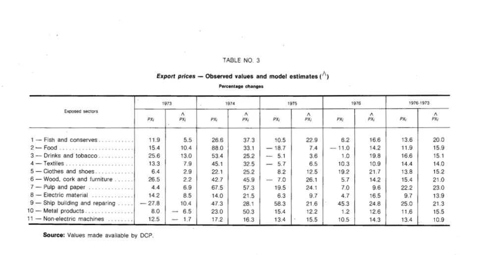
TABLE NO. 3

Export prices-Observed values and model estimates (/1)

Percentage changes

1973 1974 1975

Exposed sectors

II II II

PX; PX; PX; PX; PX; PX;

1 - Fish and conserves ... 11.9 5.5 26.6 37 3 10.5 22.9

2 -Food ... 15.4 10.4 88.0 33.1 -18.7 7.4

3 - Drinks and tobacco ... .. 25.6 13.0 53.4 25.2 - 5.1 3.6

4 -Textiles ... 13.3 7.9 45.1 32.5 - 5.7 6.5

5 - Clothes and shoes ... 6.4 2.9 22.1 25.2 8.2 12.5

6 - Wood, cork and furniture ... 26.5 2.2 42.7 45.9 - 7.0 26.1 7 - Pulp and paper ... 4.4 6.9 67.5 57.3 19.5 24.1 8 - Electric material ... 14.2 8.5 14.0 21.5 6.3 9.7 9 -Ship building and reparing ... -27.8 10.4 47.3 28.1 58.3 21.6 10-Metal products ... 8.0 - 6.5 23.0 50.3 15.4 12.2

11 - Non-electric machines ... 12.5 - 1.7 17.2 16.3 13.4 15.5

Source: Values made available by DCP .

1976 1976·1973

II II

PX; PX; PX; PX;

6.2 16.6 13.6 20.0

-11.0 14.2 11.9 15.9

1.0 19.8 16.6 15.1

10.3 10.9 14.4 14.0

19.2 21.7 13.8 15.2

5.7 14.2 15.4 21.0

7.0 9.6 22.2 23.0

4.7 16.5 9.7 13.9

45.3 24.8 25.0 21.3

1.2 12.6 11.6 15.5

10.5 14.3 13.4 10.9

-...

en TABLE NO.4

Home market prices-Observed values and model estimates ("\)

-Percentage changes

1973 1974 1975 1976

Exposed sectors

1\ 1\ 1\

PI; PI; PI; PI; PI; PI; PI;

1 - Fish and conserves ... 19.7 4.7 43.1 47.2 6.3 24.3 22.6

2 - Food ... 14.6 2.9 57.5 56.0 7.3 20.9 11.3

3 - Drinks and tobacco ... 17.7 - 0.5 - 4.7 52.9 - 1.7 12.7 26.4

4 -Textiles ... 19.6 - 0.5 29.9 43.0 5.1 21.7 16.0

5 - Clothes and shoes ... 12.9 - 1.8 21.2 41.2 20.7 20.7 22.0 6 - Wood, cork and furniture ... 47.8 - 0.3 34.8 36.0 - 4.1 12.3 23.5

7 - Pulp and paper ... 2.5 3.4 53.6 47.5 19.9 25.5 1.4

8 - Electric material ... - 7.8 - 3.1 12.0 45.5 29.0 20.9 8.8 9 - Ship building and reparing ... -31.1 15.5 36.6 55.3 - 6.6 22.0 26.6 I 0 - Metal products ... 10.8 - 0.1 19.9 25.4 29.4 14.6 18.5 11 - Non-electric machines ... 4.7 4.3 31.0 29.0 15.8 20.8 27.6

_{_.._}

Source: Values made available by DCP.

1976·1973

1\ 1\

PI; PI; PI;

16.6 22.2 22.3

3.8 21.2 19.1

12.9 8.6 18.0

6.6 17.3 16.6

14.4 19.2 17.6

12.7 23.9 18.7

14.8 17.6 21.4

14.6 9.7 15.5

11.1 2.7 23.4

29.8 19.5 16.8

....

TABLE NO. 5

Export market shares-Observed values and model estimates (11 )

Percentage changes

1973 1974 1975

Exposed sectors

1\ 1\ 1\

MXi MXi MXi MXi MXi MXi MXi

1 - Fish and conserves . . . . ... 0.7 10.7 -23.4 - 8.6 - 3.7 - 8.6 -23.8 2 -Food ... . . . . . . 13.5 2.2 -22.0 - 4.0 -14.7 -18.5 -39.1 3 - Drinks and tobacco ... 10.6 - 0.4 14.8 -10.9 -16.0 -19.9 -17.9 4 -Textiles ... . . . . . . . . 7.1 1.4 6.0 - 4.8 -12.3 -11.5 -21.6

5 - Clothes and shoes ... 17.8 4.3 3.3 -10.2 ---: 15.8 - 8.8 -23.7 6 - Wood, cork and furniture ... 4.4 28.9 25.2 1.8 -22.6 2.1 -11.1 7 - Pulp and paper ... - 5.1 1.2 -12.7 2.3 14.8 - 2.8 12.9 8 -Electric material ... 13.2 0.3 8.1 - 3.5 - 7.5 - 0.6 - 26 .. 3 9 - Ship building and reparing ... 105.0 - 1.3 68.4 -10.1 -33.6 -10.1 - 6.5 I 0 - Metal products ... -34.1 11.0 - 7.2 -15.6 6.8 8.9 20.9

11 - Non-electric machines ... 9.5 - 4.4 - 3.7 -10.0 - 8.4 - 7.0 -14.8

-'---

-Source: Values made available by DCP .

1976 1976·1973

1\ 1\

MXi MXi MXi

- 1.4 -13.11 - 2.28

- 9.3 -17.65 - 7.72

- 9.7 - 3.27 - 10.49

- 2.1 - 6.01 - 4.37

- 0.1 - 5.97 - 3.89

8.1 - 2.62 9.7

- 2.2 1.8 - 0.4

1.8 - 4.4 - 0.52

-17.0 20.9 - 9.8

9.8 - 5.7 2.9

b) Over and underestimation

The number of estimates corresponding to over and underestimation is shown in table no. 6, in which the number of estimates involving errors related to the sign of the variable (turning point errors) (18

) is also specified.

1973

Variables

0 u

PX ... 2 9

PI ... 3 8

MX ... 4 7

Total 9 24

TABLE NO.6

Frequency of over (o) and under (u) estimation and turning point errors (tpe)

1974 1975 1976

tpe 0 u tpe 0 u tpe 0 u

3 5 6 9 2 4 10 1

6 7 4 1 9 2 3 3 8

4 3 8 6 6 5 2 8 3

13 15 18 7 24 9 9 21 12

Total -1973·1976

tpe 0 u tpe

1 26 18 8 22 22 10 3 21 23 15 4 69 63 33

A tendency towards underestimation may be observed in the years 1973-197 4, while for 1975-1976 the model results often involved overestima-tion errors. As it is known, due to the increases in oil prices, price develop-ments in 1973-1974 were generally much higher than the traditional fore-casting tools would predict. The political changes occurred in Portugal in 197 4 also had a significant impact on cost and price developments. It is, therefore, not surprising that the model's structure and basic assumptions led to price changes in these years which were lower than the observed ones. On the other hand, underestimation of price variables would have re-sulted in overestimation of the changes in export market shares. As this was not the case, one may conclude that inadequate elasticities and/or lag structures were used or that the model's relations are not appropriate to explain market share developments.

For the years 1975-1976, when economic developments were probably more in line with structural trends, the high frequency of overestimation . may also be related to inadequate parameter values or to inappropriate ba-sic assumptions in the model.

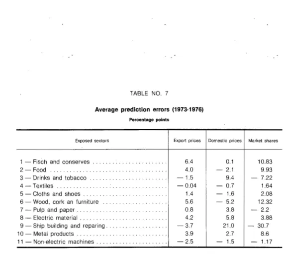
c) Average prediction errors

The ability of the model in forecasting may also be evaluated through the value of prediction errors (difference between estimates and observed values). Table no. 7 indicates the average errors (19

) for the period 1973-·1976.

(18) See Theil's Applied Economic Forecasting, North Holand, 1966.

TABLE NO. 7

Average prediction errors (1973-1976)

Percentage points

Exposed sectors

1 - Fisch and conserves ... . 2 - Food ... . 3 - Drinks and tobacco

4 -Textiles . . . . ... . 5 - Cloths and shoes ..

6 - Wood, cork an furniture 7 - Pulp and paper ...

8 - Electric material . . . . ... . 9 - Ship building and reparing . . . . . ... . 10 - Metal products . . . . . ... . 11 - Non-electric machines ... .

Export prices

6.4 4.0 -1.5 -0.04 1.4 5.6 0.8 4.2 -3.7 3.9 -2.5

Domestic prices

0.1 2.1 9.4 - 0.7 - 1.6 5.2 3.8 5.8 21.0 2.7 - 1.5

Source: Calculated on the basis of values inclued in tables nos. 3, 4 and 5.

Market shares

10.83 9.93 7.22 1.64 2.08 12.32 - 2.2 3.88 - 30.7 8.6 - 1.17

As may be seen, the model estimates involved lower errors for the price variables than for the market share ones. In the case of the market shares, the large overestimation bias registered for sectors, 1, 2, 6 and 10 support the above mentioned conclusion that parameter values being used may be not addequate. In addition, one should keep in mind that the MCE model does only explain the changes in market shares which result of changes in relative prices. However, changes in market shares may also result from changes in the product mix of import demand over the business cycle, or even in the long run. This may be the case here, as the model is a rather aggregate one and each sector includes various commodities, for which demand may develope differently. For sector 9 the model results seem to be particulary bad. This is a very special sector -ship building and reparing- and the model's basic assumptions do probably not fit in this sector's price behaviour and export performance.

d) Errors related to the normal intensity of change of the variables

In order to mark the errors independent of special events and of the size of the variable, we will also use an accuracy indicator which relates the errors with the socalled «normal intensity of change)) of the variables (20). This indicator is zero in case of perfect estimation. It has no upper limit and it equals the unity whenever prediction corresponds to no change extrapolation.

(20) See Theil, op. cit.

Values higher than the unity may mean that extrapolation would have been a better estimation tool than the model.

Table no. 8 presents the values obtained for this indicator in the period, by sectors A) and by years B). The best results correspond to the export price variables. In this case, the global indicator (averaging all sectors and ali years) shows that the errors involved in the model estimates were 66 per cent of the errors associated to simple extrapolation. For the exporting sectors 4, 5 and 7 this percentage was, respectively, 38, 22 and 17. Results obtained for 1975-1976 were better than the ones for 1973-1974.

TABLE NO.8

Errors related to the normal intensity of change of the variables (*) (1973-1976)

A) By sectors

Exposed sectors Export prices Domestic prices Market shares

1 - Fish and conserves ... . 0.65 0.47 1.02

2 -Food ... . 0.72 0.32 0.75

3 - Drinks and tobacco ... . 0.64 1.97 0.98

4 -Textiles 0.38 0.78 0.87

5 - Cloths and shoes ... 0.22 0.66 0.92

6 -Wood, cork an furniture .... 0.82 0.82 1.28

7 - Pulp and paper .... . 0.17 0.28 118

8 - Electric material .... . 0.72 1.06 1.07

9 - Ship building and reparing . 0.65 1.08 1.04

1 0 - Metal products ... . 1.15 0.96 0.96

11 - Non-electric machines . 0.55 0.24 1.01

Total .... 0.66 0.90 1.02

(•) See appendix for the definition of the indicators.

8) By years

Years Export prices Domestic prices I Market shares

1973 ... . 0.64 0.90 1.13

1974 .. 0.82 1.31 1.07

1975 ... . 0.59 0.63 0.66

1976 ... ·'· .. 0.56 0.47 1.19

1973-1976 .. 0.66 0.90 1 02

as compared to extrapolation. Quite good results were, however, obtained again for sector 7 and also for sectors 2 and 11. Results for the year 1975 may also be considered rather good.

Finally, results are particularly disapointing for the market share variables, where in most cases the model leads to estimates as good as, or even worse, the ones corresponding to extrapolation. As it was already mentioned, in the case of the export market share equations, there may be other factors, wich are not considered in the model's present version (as changes in the demand mix), having a significant impact on market share developments.

6 - Concluding remarks

The evaluation here made was based on a very limited number of observations and for a period during which very special developments (both in Portugal and in the world markets) took place.

Definite conclusions are, therefore, difficult to draw from the available information.

The analysis of model results seems to indicate that the model is a better tool in forecasting price variables than in forecasting export market shares. In particular, relatively good results were obtained for prices in important export sectors (sectors 4,5 and 7). For the remaining sectors, there may be a room for adjusting the coefficients of the price equations, namely by improving the empirical basis of these parameters when data for a longer period becomes available. In the export market share relations, it seems that other explanatory variables, not included in the present version of the model, are also relevant. An analysis of the effects of changes in the product mix of foreign demand may be useful in determining the relative contribution of price and non-price factors affecting market shares. The model is presently used in medium-term forecasting in connection whit the macroeconomic model MODEP. The use of the model could be extended to targeting purposes (by changing exogenous into endogenous variables and vice versa) and to simulation analysis. In the first case it would be possible to determine the change in one or more instrument variables which was needed to achieve a given change in a target variable.

APPENDIX

A) List of variables and parameters

22

The model contains the following variables:

WOi(i=1 Yi(i=1 ZXi(i=1

ZMi(i=1 ZMMi(i=1 H ....

Wi(i=1 Pli(i= 1 PXi(i=1 Pi(i=1

Ci(i=1

Exogenous variables:

12) -Changes in (nominal) wage rates in sector i; 12) -Changes in productivity in sector i;

11)- Changes in international prices of products corresponding to sector i;

12) - Changes in import prices of products competing with sector i; 12) - Changes in import prices for imported inputs to sector i;

-Changes in the ratio between profits and wages in sector 12. [This variable may be determined accoording to trend values given by a line h = f (time).].

Endogenous variables:

12) - Changes in unit wage costs in sector i;

12) - Changes in domestic prices of sector i;

11) - Changes in export prices of sector i;

12) -Changes in sector i's average prices (for sector 12, P12 = P1,2);

12) -Change in unit current costs in sector i; WRiU= 1 ... 12)- Changes in sector i's real wages; PC . . . -Changes in consumer price index;

QX i(i = 1 ... 11) -Changes in relative export prices for sector i (changes in com-petitive position abroad);

QMi(i=1

MXi(i=1 MMi(i=1

BXi(i=1 Bli(i=1 aii(i.i= 1

aiMU=1 aiLU= 1

smi(i=1 SXj(i= 1

I iiU= 1

ViU= 1

Oi(i=1

11)- Changes in relative domestic prices for sector i (changes in competitive position at home);

11) - Changes in export market shares; 11)- Changes in import shares;

Coefficients:

11)- Cost incidence in export prices of sector i;

12)- Cost incidence in domestic prices of sector i; 12)- Input-output coefficients;

12)- Imported inputs per unit of sector i's production; 12)- Wage costs per unit of sector i's production; 11)- Import share price elasticity in sector i;

11)- Export market share price elasticity in sector i; 12)- Proportion of exports in sector i's total production; 12)- Each sector's weight in consumer price index;

12) - Proportion of costs in gross value of production of sector i:

lk . . . - Lag structure for relative export prices;

B) Determination of Theil's accuracy indicators (21)

For each year and each sector an accuracy indicator may be defined C!S:

Ui,t

where:

Di,t

sRi

Di, 1 is the difference between the estimate and the observed value of the variable for the sector i in the year t;

SRi is the root mean square of the observed values R i,t in the period

sRi = ( _1_ L R2 ) 112

T t i, t

and it is intended to measure the normal intensity of change over period of the variable in sector i.

A global indicator for each sector may be then defined, as:

u

i

= (

_l _T L U2 ) 112

I, t

and for each year as Ut =

c:

L Ur. 1 ) 112

and a total indicator, covering all m sectors and all T years may be obtained through:

U

= (

~

L Ur

f

12

= (

~

L Uf

f

12

Errors related to the normal intensity of change of the variables (SRi)(*)

1) Export prices

·SRi Ui

Sectors 1973 1974 1975 1976

-1973·1976

1 - Fish and conserves. .... . ... 15.80 -0.41 0.68 0.78 0.66 0.65 2 -Food ... ... 45.94 -0.11 -1.20 0.57 0.55 0.72 3 -Drinks and tobacco ... · .. 29.72 -0.42 -0.95 0.29 0.63 0.64 4 -Textiles. ... 24.24 -0.22 -0.52 0.50 0.02 0.38 5 - Cloths and shoes ... 15.53 -0.23 0.20 0.28 0.16 0.22 6 -Wood, cork and furniture ... 25.53 -0.95 0.13 1.30 0.33 0.82 7 - Pulp and paper ... 35.37 O.D? -0.29 0.13 0.07 0.17 8 -Electric material ... .... 10.72 -0.53 0.70 0.32 1.10 0.72 9 -Ship building and reparing . ... 45.99 0.83 -0.42 -0.80 -0.45 0.65 10-Metal products ... 14.42 -1.01 1.89 0.22 o.79 I 1.15

11 - Non-electric machines ... 13.62 -1.04 O.D? 0.15 0.29 i 0.55

Total Ut ... 0.64 0.82 0.59 0.56 0.66

(•) As the indicators Ui and Ut are root mean squares they are always positive.

21 Domestic prices

U;

Sectors SRi 1973 1974 1975 1976 -1973-1976

1 - Fish and conserves ... 26.44 -0.57 0.16 0.68 -0.23 0.47 2 -Food ... 30.42 -0.38 -0.05 0.45 -0.25 0.32 3 - Drinks and tobacco ... 16.09 -1.13 3.58 0.89 -0.84 1.97 4 -Textiles ... 19.75 -1.02 0.66 0.84 -0.48 0.78 5 - Cloths and shoes ... 19.55 -0.75 1.02 0.00 -0.39 0.66 6 -Wood, cork and furniture ... 31.88 -1.51 0.04 0.51 -0.34 0.82 7 - Pulp and paper ... 28.62 0.03 -0.21 0.20 0.47 0.28 8 - Electric material ... 16.76 0.28 2.00 -0.48 0.35 1.06 9 - Ship building and reparing ... 27.65 1.69 0.68 1.03 -0.56 1.08

1 0 - Metal products ... 20.73 -0.53 0.27 -0.71 0.55 0.96

11 - Non-electric machines . .' ... 22.33 -0.02 -0.09 0.22 -0.42 0.24

Total Ur ... 0.90 1.31 0.63 0.47 0.90

- ·

31 Market shares

Sectors SRi 1973 1974 1975 1976 -u;

1973-1976

1 - Fish and conserves ... 16.79 0.60 1.39 -0.29 1.33 1.02 2 -Food ... 24.55 -0.46 0.73 -0.15 1.21 0.75 3 - Drinks and tobacco ... 15.06 -0.73 -1.71 -0.26 0.54 0.98 4 -Textiles ... 13.27 -0.43 -0.81 0.06 1.47 0.87 5 - Cloths and shoes ... 16.87 -0.80 -0.80 0.41 1.40 0.92 6 - Wood, cork and furniture ... 17.95 1.36 -1.30 1.38 1.07 1.28 7 - Pulp and paper ... 11.97 0.53 1.25 -1.47 -1.26 1.18 8 - Electric material ... 15.71 -0.82 -0.74 0.44 1.79 1.07 9 - Ship building and reparing . ... 64.95 -1.64 -1.21 0.36 -0.16 1.04 10 - Metal products .. ... 20.60 2.16 -0.41 0.10 -0.54 0.96

11 - Non-electric machines ... 9.92 -1.40 -0.64 0.14 1.30 1.01

Total Ur ... 1.13 1.07 1.66 1.19 1.02

~

1972=100

1973

II

Exposed sectors PX PX

1 - Fish and conserves ... 111.9 105.5 2 - Food .... . . . . . . . . . . . . .... .. 115.4 110.4 3 - Drinks and tobacco ... ... 125.6 113.0 4 -Textiles ... 113.3 107.9 5 - Cloths and shoes ... 106.4 102.9 6 - Wood, cork and furniture ... 126.5 102.2 7 - Pulp and paper ... ... 104.4 106.9 8 - Electric material ... 114.2 108.5 9 - Ship building and reparing ... 72.2 110.4 10 - Metal products ... 108.0 93.5 11 - Non-electric machines ... 112.5 98.3

-Source: Values presented in tables nos. 3 and 4.

Export price index

1974 1975

II II

PX PX PX PX

141.7 144.9 156.5 178.0 217.0 146.9 176.4 157.8 192.7 141.5 182.9 146.6 164.4 143.0 155.0 152.3 129.9 128.8 140.6 144.9 180.5 149.1 167.9 188.0 174.9 168.2 209.0 208.7 130.2 131.8 138.4 144.6 106.4 141.4 168.4 172.0 132.8 140.5 153.3 157.7 131.9 114.3 149.5 132.0

Home market price index

1976 1973 1974 1975 1976

II II II II II

PX PX PI PI PI PI PI PI PI PI