Modeling of Laser wakefield acceleration in Lorentz
boosted frame using EM-PIC code with spectral solver
Peicheng Yua, Xinlu Xub, Viktor K. Decykc, Weiming Ana, Jorge Vieirad,
Frank S. Tsungc, Ricardo A. Fonsecad,e, Wei Lub, Luis O. Silvad, Warren B.
Moria,c
aDepartment of Electrical Engineering, University of California Los Angeles, Los
Angeles, CA 90095, USA
bKey Laboratory of Particle and Radiation Imaging of Ministry of Education,
Department of Engineering Physics, Tsinghua University, Beijing 100084, China
cDepartment of Physics and Astronomy, University of California Los Angeles, Los
Angeles, CA 90095, USA
dInstituto Superior T´ecnico, Lisbon, Portugal
eISCTE - Instituto Universit´ario de Lisboa, 1649–026, Lisbon, Portugal
Abstract
Simulating laser wakefield acceleration (LWFA) in a Lorentz boosted frame in which the plasma drifts towards the laser with vb can speedup the
simu-lation by factors of 2
b = (1 vb2/c2) 1. In these simulations the relativistic
drifting plasma inevitably induces a high frequency numerical instability that contaminates the interested physics. Various approaches have been proposed to mitigate this instability. One approach is to solve Maxwell equations in Fourier space (a spectral solver) as this has been shown to suppress the fastest growing modes of this instability in simple test problems using a simple low pass or “ring” or “shell” like filters in Fourier space. We describe the develop-ment of a fully parallelized, multi-dimensional, particle-in-cell code that uses a spectral solver to solve Maxwell’s equations and that includes the ability to launch a laser using a moving antenna. This new EM-PIC code is called UPIC-EMMA and it is based on the components of the UCLA PIC frame-work (UPIC). We show that by using UPIC-EMMA, LWFA simulations in the boosted frames with arbitrary b can be conducted without the presence
of the numerical instability. We also compare the results of a few LWFA cases for several values of b, including lab frame simulations using OSIRIS,
Email address: [email protected] (Peicheng Yu)
a EM-PIC code with a finite di↵erence time domain (FDTD) Maxwell solver. These comparisons include cases in both linear and nonlinear regimes. We also investigate some issues associated with numerical dispersion in lab and boosted frame simulations and between FDTD and spectral solvers.
Keywords: Particle-in-cell, plasma simulation, laser wakefield accelerator, boosted frame simulation, spectral solver, numerical Cerenkov instability 1. Introduction
Laser wakefield acceleration (LWFA) o↵ers the potential to construct compact accelerators that has a numerous potential applications including the building blocks for a next generation linear collider and being the driver for compact light sources. As a result, LWFA has attracted extensive inter-est since it was originally proposed [1], and the last ten years has seen an explosion of experimental results. Due to the strong nonlinear e↵ects that are present in LWFA, developing predictive theoretical models is challenging [2, 3]; therefore numerical simulations are critical. In particular, particle-in-cell (PIC) simulations play a very important role in LWFA research because the PIC algorithm follows the self-consistent interactions of particles through the electromagnetic fields directly calculated from the full set of Maxwell equations. Using a standard PIC code to study a 10 GeV stage in a non-linear regime takes approximately 1 million core hours on today’s computers and a 100 GeV stage would take 100 million core hours. While computing resources now exist to do a few of such simulations, it is not possible to do parameter scans in full three-dimensions. Therefore, reduced models such as combining the ponderomotive guiding center with full PIC [4] for the wake or with quasi-static PIC [5, 6] are used for parameter scans. However, while these models are very useful, they cannot model full pump depletion distances and the quasi-static approach cannot model self-injection. Another reduced model that has been recently proposed is to expand the fields in azimuthal mode numbers and truncate the expansion [7]. This can reduce modeling a 3D problem with low azimuthal asymmetry into the similar computational cost as using a 2D r z code.
Recently, it was shown that by performing the simulation in an optimal Lorentz boosted frame with velocity vb, the time and space scales to be
resolved in a numerical simulation may be minimized [8, 9, 10]. The basic idea is that in the boosted frame the plasma length (the laser propagation
distance) is Lorentz contracted while the plasma wake wavelength and laser pulse length are Lorentz expanded. The number of laser cycles is an invariant (assuming there is no reflected wave) so the necessary number of cells needed to resolve the laser is also an invariant while the cell size and hence time step are Lorentz expanded. The increase in time step and decrease in the plasma length lead to savings of factors of b2 = (1 vb2/c2) 1 as compared to a lab frame simulation using the so called moving window [11]. Using such simulations, it has been shown that using a 1–3 PW laser one could generate 10 GeV electron beam in a self-guided stage and 50 GeV in a channel guided stage [9]. For these cases the savings can be larger than factors of 104.
However, in the boosted frame LWFA simulations noise from a numerical instability can be an issue. As discussed in [12, 13, 14, 15, 16, 17], the noise results from a numerical Cerenkov instability induced by the plasma drifting with relativistic speeds on the grid. According to the dispersion relation this numerical instability is attributed to the coupling between the wave-particle resonances with EM modes (including aliased modes) in the numerical system. The pattern of the instability in Fourier space can be found at the intersections of the EM dispersion relation of the solver used in the simulation algorithm, and the wave-particle resonances [15, 16, 17].
In order to mitigate this instability, it is preferable to use an EM solver that eliminates the numerical instability at the main beam resonance. In this case, the instability occurs only at high |~k| modes which are far away from the physics of interest. As the EM dispersion curves for most FDTD solvers inevitably bends down (i.e., supports waves with phase velocities less than the speed of light) at high|~k|, numerical instabilities at the main beam resonance are found in these solvers. However, when using a spectral solver that spatially advances the EM fields in Fourier space, the dispersion curve assures no instability pattern at the main beam resonance. In addition, the pattern at the first space aliasing beam mode is found to indeed be located at high |~k| values that are far away from the interested physics. For the spectral solver the numerical Cerenkov instability is located at a predicted pattern in ~k space so it can be conveniently eliminated by applying simple filters directly in ~k space.
In this paper we describe the development of a fully parallelized three-dimensional electromagnetic spectral PIC code called UPIC-EMMA that was rapidly built using components of the UCLA PIC Framework (UPIC) [21]. We demonstrate that through the use of appropriate filters, Lorentz boosted
frame simulations of LWFA at the optimum frame velocities can be carried out without limitations from the numerical Cerenkov instability. We show that a simple low pass filter with a hard cuto↵ at |~k| works very well. This completely eliminates modes with |~k| above a selected value. Meanwhile, it is not as easy to use such a filter in|~k| space using a FDTD solver (and such solvers have instabilities at lower |~k|).
As discussed in Ref. [16, 17], when using the FDTD code to simulate relativistic plasma drift, an optimized time step has to be chosen to minimize the instability growth rate. While the instability growth rate is minimized, this time step does not lead to complete elimination of the instability and it can lead to further errors in numerical dispersion. Additional smoothing and filtering can help as well, but unlike when using a spectral code the instability cannot be essentially eliminated. For the spectral code, the only errors in numerical dispersion arise from the use of finite time step. Because, it is not necessary to use an optimum time step (nor does one exist), one can minimize the errors in numerical dispersion for the EM waves by choosing smaller time steps if needed. One disadvantage with the spectral code is that it is not easy to use a moving window, however for the optimum bno moving
window is needed. We note that the use of a pseudo-spectral algorithm has recently been discussed and analyzed [23]. This can easily be included into UPIC-EMMA if the algorithm is shown to have advantages.
We have benchmarked UPIC-EMMA by comparing the 2D and 3D sim-ulation results of LWFA in Lorentz boosted frames with the corresponding OSIRIS [26] lab frame simulations. Good agreement is found between the OSIRIS lab frame simulations, and UPIC-EMMA boosted frame simulations, in both linear, and nonlinear regimes. We also compare UPIC-EMMA sim-ulations for di↵erent values of b and excellent agreement is found.
The remainder of this paper is organized as follows. In section 2 we dis-cuss the numerical instability induced by relativistic drift. In section 3, we describe the development of UPIC-EMMA, and how using the algorithms in UPIC-EMMA can eliminate the instability induced by relativistic plasma drift. In section 4, we discuss details of LWFA Lorentz boosted frame simula-tions using UPIC-EMMA. In section 5, we benchmark UPIC-EMMA results with di↵erent b and with OSIRIS lab frame simulation. Summary is given
2. Numerical instability due to relativistic plasma drift
The numerical Cerenkov instability induced by relativistic plasma drift has been extensively studied in [16, 17]. In a PIC system, when the plasma is drifting relativistically, the velocity of the drifting particles can be equal (be in resonance) to the component of the phase velocity of the main EM mode along the drift direction. In addition, its aliased modes can always be in resonance with the EM modes. The resulting wave-particle resonance leads to a violent numerical instability known as the numerical Cerenkov instability. Due to the nature of wave-particle resonances, the numerical in-stability occurs at the intersections of the beam resonances and EM modes determined by the Maxwell solver used in the simulation. By carefully choos-ing the Maxwell solver, the instability pattern can be manipulated so that mitigation can be achieved. As discussed in [12, 14, 15, 17], when a spectral solver is used, there are no intersections of the EM modes with the main beam resonance. As a result, the instability can be found only at the aliased resonances and the fatest growing modes are the first spatial aliases. These resonances reside at high |~k| in Fourier space far away from the important physics.
The instability pattern for the spectral solver can be found by investigat-ing the correspondinvestigat-ing dispersion relation,
([!]2 [~k]E· [~k]B+ [~k]E[~k]B) ~E = !2p X µ,~⌫ ( 1)µ ⇢Z S! j( ~k0)~pd~p !0 ~k0· ~p ⇢ [!]S!E(!0, ~k0) ~E + ~p ⇥ {S!B(!0, ~k0)([~k]E ⇥ ~E)} · @fn 0 @~p where ! and ~k are the frequency and wavenumber of the modes in the
simu-lation system; ~p and are the momentum and Lorentz factor of the drifting plasma; ~E is the electric field; fn
0 = (p1 p0) (p2) (p3) is the normalized
distribution function of the plasma; !p is the plasma frequency; S!E, S!B, and
!
Sj are the corresponding interpolation tensors for EM fields and current; [!]
and [~k]E,B are the finite di↵erence time and space operators for the Maxwell
solver used in the algorithm. And !0 = ! + µ!g !g = 2⇡ t µ = 0,±1, ±2, . . . k0i = ki+ ⌫ikgi kgi= 2⇡ xi ⌫i = 0,±1, ±2, . . .
where t and xi are the time step, and grid sizes in the simulation. The
sum over µ and ~⌫ is attributed to the finite grid size and time step used in the simulation. Specific expressions of [!] and [~k] can be found in Appendix A of Ref. [17].
Since the instability pattern is found near the intersections of the EM modes and beam resonance [17], we can obtain a simple analytical expression for the instability pattern in the limit t! 0 (which leads to [!] = !). Under this assumption, the equation for the EM dispersion curves in the spectral solver is
!2 ⇡ k12+ k22 And the equations for the beam resonances are
! + µ!g = (k1+ ⌫1kg1)
where ⌘ v/c. Defining ⇠ ⌘ ⌫1kg1 µ!g, we can obtain the expressions
for the intersections as
(1 2)k12+ k22 2 ⇠k1 ⇠2 = 0 (1)
Note that there are no solutions for µ = ⌫1 = 0 for the spectral solver. The
lowest order terms for the instability pattern are at the µ = 0 and ⌫1 =±1
resonances. In the limit of interest ! 1, we obtain
k22⌥ 2k1kg1 kg12 = 0 (2)
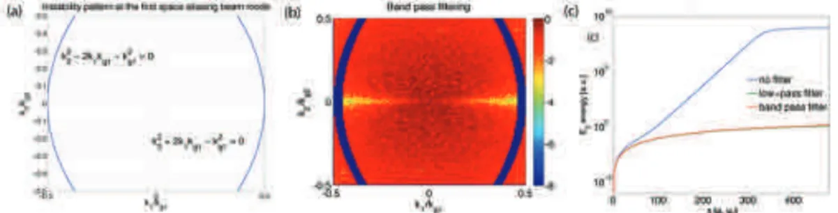
In figure 1 (a) we plot Eq. (2) for µ = 0 and ⌫1 =±1. Note the “ring” pattern
of the instability, which crosses the k2 = 0 axis near the point (±kg1/2, 0);
therefore this mode is located at high |~k| values which are far away from the region of interesting physics. Therefore, the numerical Cerenkov instability can be e↵ectively eliminated if the fatest growing modes (µ = 0, ⌫1 = ±1)
are suppressed in the Maxwell solver.
In the simulations, we identify the unstable modes in Fourier space using the approximate expression Eq. (2). We then apply filters with specific masks which multiply the undesired modes by zero. In figure 1 (b) we plot the “ring-shaped” band-pass filter used in some of the two-dimensional simulations for testing the instability mitigation. We put “ring” in quotes because it is not true ring but rather a range between two parabolas. We also used a low
pass filter with a hard cut-o↵. We filled the simulation box with neutral plasma drifting relativistically at = 14000 in the x1 direction, and ran
cases without a filter, with the “ring” filter, and the low pass filter with a hard cuto↵. As seen from figure 1 (c), these filters efficiently suppresses the instability modes at µ = 0, ⌫1 =±1 in E2 [17]. Therefore, the mitigation of
the instability using band-pass filters shows the flexibility and efficiency of a spectral solver in being able to pinpoint the suppression of the unphysical modes in PIC simulations while leaving the modes near the interesting physics completely una↵ected.
3. EM-PIC code with spectral solver
As mentioned in the section 2, an EM-PIC code with a spectral solver has superior properties in suppressing the numerical Cerenkov instability induced by a relativistic plasma drift. They also have superior properties with respect to numerical dispersion errors and noise. In the following, we will briefly explain the algorithm of a spectral EM-PIC code, as well as discuss the challenges in optimizing the performances of such a code.
Spectral PIC codes have a long history [18]. However, despite their ad-vantages in better accuracy and less noise, they are not currently as widely used because they use global field solvers which do not scale as well on par-allel computers, and implementing boundary conditions is not as straight forward. A spectral EM-PIC code has the same basic flow chart as a finite-di↵erence-time-domain (FDTD) PIC code. In a spectral EM-PIC code both the charge and current are deposited on the mesh from the particles; the forces exerted on the particles are interpolated from the mesh points, and particles are advanced using the Lorentz forces. The main di↵erence between the spectral PIC code and FDTD PIC code is the solver used to advance the electromagnetic field and that all field quantities, including the charge and current densities, are defined at the same locations on a cell (no Yee mesh [19] is needed). In a spectral PIC code the charge and current are directly de-posited, and a strict charge conserving current deposit is not needed because Gauss’s law is solved at each time step using the charge density. This gives the longitudinal part of the electric field. The longitudinal component of the magnetic field is set to zero at each time step. Faraday’s law and Ampere’s law are used to advance the transverse electric and magnetic fields forward in time. Note that because Gauss’s law is solved for directly at each time step, a charge conserving current deposit or Boris correction to the longitudinal
component of the electric field is not required to maintain that Gauss’s law is satisfied. The equation for the longitudinal component of electric field ~EL
becomes:
~
EL(~k) = 4⇡⇢(~k)
i~k
k2 (3)
and the transverse electric field and magnetic field are leap-frogged forward in time using Faraday’s and Ampere’s law:
@ ~ET(~k)
@t = ic~k⇥ ~B(~k) 4⇡~jT(~k)
@ ~B(~k)
@t = ic~k⇥ ~ET(~k) (4) where the transverse component of the current is:
~jT = ~j ~k(~k ·~j)
k2 (5)
We also multiply ⇢(~k) and ~J(~k) by a shape function S(~k) = exp( |k|2a2/2)
where a is the particle size. The fields are also multiplied by this shape function then interpolated to the particles [18].
In addition, just as in a FDTD code, the particle positions and velocities (and correspondingly the charge and current densities) are defined at half integer values in time with respect to each other. If positions are defined at whole time steps and velocities (momentum) at half integer values, then the longitudinal and transverse components of the electric field are defined at whole time steps (when particle positions are defined) and the magnetic field is defined at half-integer values. Once the fields are transformed back from ~k space to real space then the particles can be pushed. The particle push is identical to that of a FDTD except for the interpolation of the forces because all field quantities are defined at the same locations in a cell.
There are no dispersion errors for light waves due to the grid, however there are errors from the time step. This is a significant advantage of the spec-tral solver, whereas a FDTD code describes the [k]i operator to O(ki xi)3,
the spectral code has no errors in the [~k] operator. Both a spectral and a FDTD code e↵ectively truncate the highest |ki| to ⇡/ xi. In addition, when
including time step errors, the numerical dispersion of a spectral PIC code is superluminal, while that of the FDTD code is subluminal. A pseudo-spectral algorithm which also removes the time step errors has recently been described
[23]. As we discuss elsewhere in this paper, the more accurate and superlu-minal aspect of the EM dispersion relation provided by the spectral solver (together with the simple filters) is crucial for eliminating the fastest growing modes of numerical Cerenkov instability. This ensures no non-physical inter-action between waves and particles in the first Brillouin zone for the spectral PIC code. The corresponding Courant condition in 2D and 3D are (for the square and cubic cells) [18]:
t2D = 2 p 2⇡c t3D = 2 p 3⇡c (6)
A spectral PIC code is also distinguished from a FDTD code in the way it is parallelized. For the field solver, the simulation box is usually partitioned in one dimension in 2D, and two dimensions in 3D, so that each processor holds global information in the dimension to be transformed. As a result, a parallel spectral PIC code requires a fast parallel transpose routine to accomplish efficient FFT in multi-dimensions. The nature of all-to-all communications in the FFT routines makes it challenging for spectral PIC code to scale to large number of processors [20]. In many cases the decomposition for the particles is the same as that for the fields although this does not have to be the case.
We have developed a multi-dimensional EM-PIC code using a spectral field solver called UPIC-EMMA. This code was rapidly put together using components provided by the UPIC Framework, a PIC framework with spec-tral solvers developed at UCLA [21]. UPIC-EMMA is fully relativistic and fully parallelized. Inherited from the UPIC Framework, UPIC-EMMA is coded in layers for convenient extension with di↵erent programming styles. The lowest layers are written in Fortran77 for high performance. They can be easily extended to many other languages. On top of this layer exists a library of Fortran90 wrapper functions which hide the complexity of the Fortran77 layer and that provide simpler arguments which enables strict type checking. The code separates the physics procedures from the communication, and uti-lizes the Message-Passing Interface (MPI) for parallel processing. In addition, a multi-tasking library was implemented to enable mixed multi-tasking and MPI messaging, where multi-tasking is used on a multiple CPU shared mem-ory node, and message-passing is used between such nodes. UPIC-EMMA also features 3D load balancing where the fields and particles use di↵erent partitions.
4. LWFA Simulations in the Lorentz boosted frame
In section 2 we described general issues regarding numerical instability that arises when a plasma drifts near the speed of light. In this section we describe some details regarding issues specific to modeling LWFA in a Lorentz boosted frame. We describe issues related to numerical dispersion in the lab frame, in the boosted frame, and in transforming from the boosted frame back to the lab frame for comparison. We also discuss the moving antenna and interactions between the laser and the drifting plasma boundary.
4.1. Numerical dispersion errors for the laser
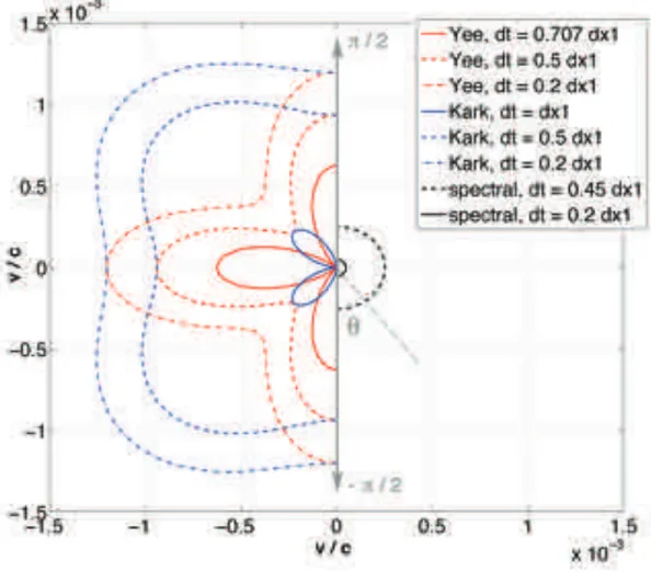
As mentioned in the introduction, one of the first obstacles in modeling LWFA in a boosted frame is to mitigate the numerical Cerenkov instabil-ity. For the FDTD PIC code [16, 17] which uses a combination of a Yee solver together with the momentum conserving field interpolation scheme, it is useful to choose the optimal time step t ⇡ x1/2, where ˆ1-direction is
the plasma drifting direction, to minimize the numerical Cerenkov instabil-ity growth rate. The need to use this time step eliminates the flexibilinstabil-ity in tuning the time step to minimize numerical dispersion errors for the laser. In figure 2 we present the error in group velocity of an EM wave on a grid in 2D (we let x1 = x2). Note that for the Yee, and Karkkainen solvers [22]
which were discussed in Ref. [16, 17], the most accurate dispersion relation occurs at their Courant Limit, but not the corresponding optimal time step at t⇡ x1/2 (for momentum conserving field interpolation). On the other
hand, for a spectral PIC code the instability mitigation does not rely on the relation of grid sizes and time step. In particular, the EM dispersion rela-tion can be made arbitrarily accurate by reducing the time step [see figure 3 (a)]. Therefore, in general when simulating relativistically drifting plasma, a spectral PIC code can provide more accuracy and flexibility over the FDTD PIC code with respect to numerical dispersion in the simulated frame. Note that recently in Ref. [23] a pseudo-spectral algorithm is described which can further improve the accuracy.
4.2. Lorentz transform of boosted frame data
While numerical dispersion errors exist when using a finite size grid in vacuum, here we show that when modeling the LWFA in the Lorentz boosted frame, these errors in the boosted frame are not necessarily an issue when the results are transformed back to the lab frame. While the value for b in
the boosted frame can be arbitrary, the speed up is generally larger as b is
increased. However, choosing b ⇡ w, where w is the phase velocity of the
wake, is generally optimum because in this frame the plasma length and the laser pulse length are nearly matched. When the laser and plasma frequency are comparable each is resolved similarly, i.e., there is no over-resolution of either the laser wavelength or plasma wavelength. In the boosted frame, the length of the plasma contracts by b, the electron and ion mass are both b
times heavier, the plasma density is b times larger, and the corresponding
plasma frequency is a Lorentz invariant. As for the laser, there is a b(1 + b) stretch to the pulse length, while the Rayleigh length contracts by b.
Therefore, while the pulse waist does not change, the e↵ective spot size at the rear of the pulse increases by a factor of 2
b(1 + b). Hence for sufficiently
large b an antenna is needed to launch the laser from the laser pulse waist
that is moving backwards. The antenna is usually placed at the plasma boundary (see section 4.3 for details).
In the lab frame simulation, a moving window which only models the region of interest around the laser is often used to reduce the simulation box size. Implementation of a moving window is challenging in a spectral PIC code due to the non-local nature of the field solver which necessitates knowl-edge of boundary condition at both of the moving boundaries. However, the relative range of x1 and t contracts when Lorentz transforming the data of
interest from lab frame to boosted frame. If b is appropriately chosen, in
this frame the length of the plasma column is of the same order as the laser pulse length. As a result, for b ⇠ w it is feasible to conduct the boosted
frame simulation without the moving window.
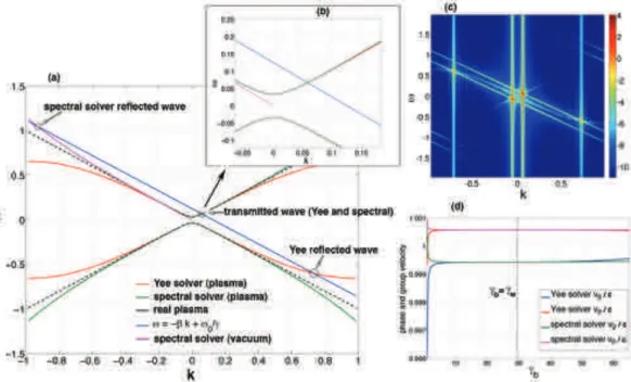
In LWFA lab frame simulations, an EM wave with frequency !0 is
inci-dent on a stationary plasma slab. This leads to a reflected and transmitted waves, each having the incident frequency. Their wave numbers are deter-mined from the dispersion relation in vacuum (reflected wave), and in plasma (transmitted wave). In a simulation the same physics occurs except the EM wave now satisfies the numerical dispersion relation in vacuum and plasma. In the boosted frame there is still a reflected and transmitted waves, except in this case the incident wave, reflected wave, and transmitted wave each have di↵erent frequencies. Furthermore, numerical issues can lead to some subtle e↵ects. An e↵ective method to identify the frequencies of the reflected and transmitted waves is to use an (!, k) diagram, which was previously used in studying the radiation generated from ionization fronts [24]. At the plasma boundary z0 = vbt, the phase of each wave = kz !t = (kvb+ !)t must
be the same, otherwise the continuity of fields cannot be satisfied at every instant in time. This leads to
kivb+ wi = krvb+ !r = ktvb+ !t (7)
where i, r, t correspond to incident, reflected, and transmitted waves respec-tively. For example, if vb = 0 then !i = !r = !t. If the incident and reflected
waves obey the vacuum dispersion relation ! = ck then !r =
1 + b!i
1 b
(8) which can also be obtained from a double Lorentz transformation. In a Lorentz boosted frame the plasma is drifting but !i = !0 is Lorentz
trans-formed to !0
i and we want !r0 and !0t [where the (0) sign refers to the boosted
frame variables]. In this frame
!0+ k0vb = !00 + k00vb (9)
where !0 can be either the reflected or transmitted waves. The constant !0
0 + k00vb is obtained by Lorentz transforming !0 and k0 into the boosted
frame: !0
0 = 0(!0 k0vb) and k00 = 0(k0 vb!0/c2). Therefore, !0+ k0vb =
!0/ b regardless of the relationship between !0 and k0. In a real system
!0 = k0c although numerical errors in the dispersion relation do not alter
the constant !0/ b. Therefore, the reflected and transmitted waves must fall
along the line !0 = k0vb+ !0/ b in (!0, k0) space (here we are ignoring the
aliasing modes). In addition, they must also fall on the dispersion curves for light in a plasma [17] [!]2 = [k]2+ ! 02 p b S2[!] [k]vb ! kvb (10) or in vacuum [!]2 = [k]2 (11)
on the grid where we assume S = Sj3 = SE3 = SB2 in Eq. (19) of Ref.
[17], and !02
p/ b = 4⇡e2n00/me is Lorentz invariant where n0 is the lab frame
density, e is the electron charge, and me is the electron rest mass. The
Eq. (10) in plasma or Eq. (11) in vacuum. This is shown in figure 3 (a) for a case where t ⇡ 0.5 x1, !0/!p ⇡ 30, and b = 8.0. The line
!0 = vbk0+ !0/ b and the dispersion curve for a real plasma (black dashed
lines), a FDTD Yee solver (red lines), and a spectral solver (green lines for inside the plasma; magenta lines for in vacuum) are shown. The vacuum dispersion relation is plotted for the spectral solver in the upper left quadrant for the reasons given in the next paragraph. In figure 3 (b), we have expanded the region in (!, k) space near the origin to illustrate the frequency and direction of the transmitted wave which does not depend strongly on the solvers used. When b = w = !0/!p then !t0 = !p = !p0/p b and k0t= 0. If b > w then !00 would be negative and the phase velocity and group velocity
of the transmitted wave would be negative; however, since |v0
gt| < |vb| the
transmitted wave would still be in the plasma.
Figure 3 (a) also illustrates that numerical errors to the dispersion relation e↵ect the location of the reflected wave. In a real system where !0 = ck0 in vacuum and !02 = !02
p / b2 + c2k02 in the plasma, then the reflected wave
would occur where !0 =
bk0 + !0/ b intersects the vacuum curve, i.e.
at !0 = !b b(1 + b) ⇠ 2! b, which is larger than the largest !0 in the
fundamental Brillouin zone. However, for the numerical dispersion curves shown in figure 3 (a), the reflected wave resides at the intersection with the plasma dispersion relation in the lower right quadrant for the FDTD solver or with the vacuum dispersion relation in the upper left quadrant for the spectral solver. For the FDTD case, the reflected wave has a negative phase and group velocity. However, the group velocity is less than vb so the
reflected wave propagates backwards while staying inside the plasma. For the spectral solver the group velocity is slightly larger than the speed of light so it resides outside the plasma. The predicted locations of the transmitted and reflected waves are confirmed in an OSIRIS (FDTD) simulation. This is seen in figure 3 (c), in which the !0 and k0 spectrum is plotted from a simulation
for parameters identical to those used to generate the theoretical plot in figure 3 (a). Strong signals are seen at the predicted locations. For cases of interest the reflection coefficient is small [the reflected signal is significantly smaller than the transmitted signal in figure 3 (c)] so the unphysical mode is not energetically important, and it does not complicate the physics.
We have also investigated the invariance of transforming results back to the lab frame based on the numerical dispersion relations. We note that solving Maxwell’s equations on a grid using discrete time steps is not strictly Lorentz invariant. For example, the group velocity of light in vacuum for
a spectral solver is greater than the speed of light, and it depends on ! t. Nevertheless, when carrying out LWFA (or other) simulations in a boosted frame, the results are transformed back to the lab frame using the Lorentz transformations. This is assumed to be reasonable if one is looking at modes which are properly resolved.
As noted earlier, when b is chosen near w there is a balance between
the laser pulse length and the plasma length. In addition, for b ⇡ w the
transmitted wave k0 ⇠ 0, and errors in the boosted frame due to the finite cell size are minimized. In figure 3 (d) we show that when v0 and v0g for the
transmitted wave are Lorentz transformed back to the lab frame using the velocity addition formulas,
= 0 + b 1 + 0 b g = 0 g+ b 1 + 0 g b (12) where and g are the phase and group velocity normalized to c, that the
numerical errors are nearly absent for sufficiently large b. The values for
v0 and v0
g are calculated from the linear dispersion relation, where ! t =
0.5k x1 is given and k x1 = 0.2 is from the dispersion relation in the lab
frame. In the boosted frame t0 =
b(1 + b) t and x01 = b(1 + b) x1.
According to the plot, for b = 1 there are clear numerical errors; however,
for b 5, the numerical errors are minimized.
These results can be understood as follows. In a Lorentz boosted frame where b = w ⌘ (1 w2)1/2, the group velocity g0 ! 0, while the phase
velocity 0 ! 1 in the numerical system, which when substituted back to Eq. (12) leads to
= 1/ w g = w (13)
which are the accurate values for a continuous system. In addition, writing = + , and 0 = 0 + 0, where and 0 corresponds to the correct
values in the lab and boosted frame, and defining
,g = 0
,g+ b
1 + 0,g b (14)
we can obtain the expressions of the error ⌘ ,g ,g as
= 1
(1 + 0 b/ 0 + b)(1 + 0
b/ 0) b2
Note the 2
b in the denominator indicates that when b is sufficiently large,
the errors in velocity when transformed back to the lab frame will be small for any waves. We also note that the arguments going from Eq. (12) to Eq. (15) hold for any velocity including those of the particles. This indicates that if we choose the b large enough that we would obtain more accurate
results compared to a simulation done in the lab frame (with typical cell sizes and time steps). An area of future work is to quantify the di↵erences more accurately.
4.3. Moving antenna
As discussed in [9] and [25], the e↵ective spot size of the laser increases by a factor of 2
b(1 + b) because the Rayleigh length of the laser contracts by b and the pulse length expands by b(1 + b). To prevent the need for using
a simulation box with transverse size ⇠ 2
b times that in needed in the lab
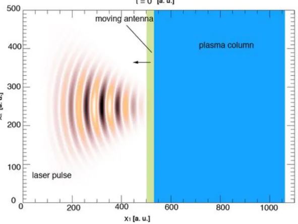
frame, we utilize a thin slice of grids at the plasma boundary (where the laser beam waist resides) as an antenna to drive the laser pulse into the plasma. The antenna is moving together with the plasma boundary [see figure 4].
The EM field in the moving antenna as a function of ~x and time t can be derived as follows (see also [9] and [25]). For instance, for a laser linearly polarized in the ˆ2 direction, the expression for the electric field E2(~x, t) of a
Gaussian pulse in the lab frame can be expressed as: E2(x1, x2, x3, t) = E0W0 W (x1) exp x2 2+ x23 W2(x 1) exp 2(x1 ct)2 2 s exp ikx1 + ik x2 2+ x23 2R(x1) iarctanx1 xR exp( i!t) with W (x1) = W0 s 1 + x 2 1 x2 R R(x1) = x1 ✓ 1 + x 2 R x2 1 ◆ xR = ⇡W2 0
where E0 is the amplitude, W0 is laser pulse waist, s is the laser pulse
length, ! and k are the laser frequency and wavenumber, and xR is the laser
Rayleigh length. A similar expression holds for the magnetic field B3(~x, t).
laser pulse in the boosted frame E20(⌘, x02, x30, t0) = E00W0 W0(⌘)exp x02 2 + x023 W02(⌘) exp 2[⌘ (1 + )ct0]2 02 s exp ik0⌘ + ik0x 02 2 + x023 2R0(⌘) iarctan ⌘ x0 R exp( i!0t0) (16) where ⌘ = x01+ bct0 s0 = b(1 + b) s E00 = E0 b(1 + b) (17) k0 = k b(1 + b) !0 = ! b x0R = xR b (18) W0(⌘) = W0 s 1 + ⌘ 2 x02 R R0(⌘) = ⌘ 1 + b ✓ 1 + x 02 R ⌘2 ◆ (19) We have neglected the fact that E2 may not equal B3 when solving for the
fields on a grid, i.e., ! 6= kc. In the spectral code, the transverse and lon-gitudinal components of the fields are solved for separately. Therefore, on the antenna we set ⇢ = 0 so there are no longitudinal fields on it. When launching a laser from the antenna, we assign current (in the direction of the laser polarization direction) at every point inside the antenna such that ~E has the desired form and polarization. The other components and the mag-netic field follow naturally from the Maxwell field solver. The antenna has a finite width of around /2 where is the wavelength of the laser in vacuum to eliminate any backward propagating signal. The current for generating the laser is added after the current is deposited for all the particles in the system is finished.
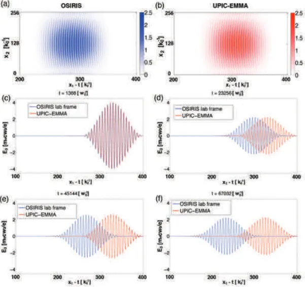
The moving antenna implemented in UPIC-EMMA is benchmarked by transforming the data back to the lab frame and then comparing it to data from an OSIRIS lab frame simulation. In the OSIRIS lab frame run, the laser propagates in the x1 direction together with the moving window; as in
the UPIC-EMMA run, the laser is launched from a moving antenna. In the UPIC-EMMA simulation b = 14 is used. Periodic boundary condition are
used for transverse directions in both cases. The transformed UPIC-EMMA boosted frame data (to the lab frame) are plotted together with the lab frame OSIRIS data in figure 5. Good agreement is found between the two cases. Note the shift in the laser wave packet between the OSIRIS data and UPIC-EMMA data. We verified that the shift was attributed to the di↵erence in
group velocity between the Yee solver and spectral solver (transformed back to lab frame).
4.4. Filters
Earlier the mode numbers of the fastest growing modes of the numerical Cerenkov instability in the spectral solver were identified as Eq. (2). Based on this equation, we use filters that eliminate a range of ~k’s centered around this parabola. Specifically, we muliply all modes by either 1 or 0. Those modes multiplied by 0 are those in the range:
k22 =±2kg1(k1+ k1) (20) in 2D, and k22+ k32 =±2kg1(k1+ k1) (21) in 3D. k1 is usually chosen to be 0.9⇥ kg1 2 < k1 < 1.02⇥ kg1 2 (22)
5. LWFA simulations with UPIC-EMMA
We next present simulation results using UPIC-EMMA to model LWFA in a boosted frame. Two-dimensional simulations in the linear and nonlin-ear regimes are presented for two di↵erent choices of b and the results are
compared to OSIRIS simulation results in the lab frame (the UPIC-EMMA results are transformed back to the lab frame). We also present 3D results from UPIC-EMMA including comparison with OSIRIS lab frame simula-tions. For the linear cases a0 = 0.1, while for the nonlinear cases a0=3.0
or 4.0. In both the OSIRIS and UPIC-EMMA simulations the time step is chosen near the Courant limit. Precise values for the simulations parameters are shown in tables 1 and 2.
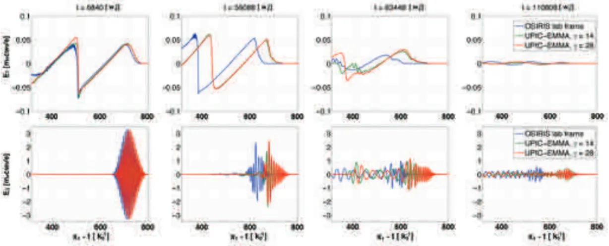
In figure 6, results from the a0=0.1 case are shown. In the top row, the
wakefield E1 is shown at various lab frame times for an OSIRIS lab frame
simulations (blue) and for two UPIC-EMMA simulations where b=14 (red)
and b=28 (green) respectively. This figure shows that for early times the
three curves are inseparable while for later times the results from OSIRIS lag behind. At later times the UPIC-EMMA results for the di↵erent b remain
inseparable. There is no evidence in these plots of any noise in the wake and laser fields due to the numerical Cerenkov instability. The fact that the OSIRIS lab frame result slips backwards is due to the numerical dispersion error in vg that was discussed earlier. In the bottom row of figure 6, the laser
field (E3) is plotted at the same times. The same colors are used to show
the results from the three simulations. The slippage of the OSIRIS lab frame curve is also seen in the laser field.
We next show results for a more nonlinear case where a0=3.0. As before,
there is a lab frame OSIRIS simulation and two UPIC-EMMA boosted frame simulations with b=14 and b=28. The same colors as in figure 6 are used to
distinguish the data from these three simulations. We plot the accelerating field in the upper row and the laser field in the lower row at four various lab frame times (di↵erent times than used in figure 6). Similarly to the linear a0 = 0.1 case the wakefields from the three simulations are inseparable at
early times while for later times the OSIRIS results slip behind. While the agreement between the two boosted frame simulations is still good, it is not as good as for the previous case. The di↵erences in the laser field are small for larger values of x1 t (at the head of the laser) and there are di↵erences
at later times.
Next in figures 8 and 9, we present results from a case where the laser amplitude is increased to a0 = 4.0. In the top row of figure 8, the plasma
density and wakefield in the Lorentz boosted frame with b = 14 are plotted
at xt0 = 6180! 1
0 . There is no evidence of the numerical Cerenkov instability.
Only a small region of the simulation box, including where the instability is most robust, is plotted. In the lower row of figure 8 we also plot in the lab frame the wakefields obtained in these three simulations. As in the two previous cases, good agreement is found in the wakefield amplitude. There is slippage of the wakefield in the OSIRIS simulation and small di↵erences between the two boosted frame simulations.
It is worth noting that, in the case where b = 28 (green), the wakefield
around the spike looks di↵erent compared with that of = 14 (red) and OSIRIS lab frame simulation (blue). The flattened part in the = 28 curve indicates more self-trapped charge is loaded in the wakefield. We believe these di↵erences may be due to di↵erent statistics since each macro-particle represents much higher charge at higher b. In the LWFA lab frame
simula-tion we usually choose the longitudinal cell sizes (along the laser propagasimula-tion direction) to be a fraction of c/!0, and the perpendicular cell size to be a
Meanwhile, in the Lorentz boosted frame the perpendicular cell size remains the same, while the longitudinal cell size increases by b(1 + b) due to the
stretch of the laser wavelength. At the same time, the plasma column con-tracts by b thus the plasma density increases by b. As a result, if we keep
the number of particle per cell to be the same as in the lab frame, factors of (1 + b) b2 savings can be achieved in the boosted frame simulation. Howver,
in this case the increase in longitudinal cell sizes and plasma density causes one macro-particle to represent (1 + b) b2 more charge then in the lab frame.
For example, if we use a cell with longitudinal size of 0.2c/!0, perpendicular
sizes of 0.2c/!p, and 8 particles per cell, for a plasma density ⇠ 1018 cm 3,
each macro-particle represent ⇠ 3.6 ⇥ 103 real electrons, which corresponds
to ⇠ 0.6 fC of charge. If b ⇠ 30, then one macro-particle in the boosted
frame corresponds to ⇠ 1.2 pC. This shows that modeling self-trapping in Lorentz boosted frames at large b will require future work including
identi-fying where the self-trapped particles come from and loading more particles per cell in these regions.
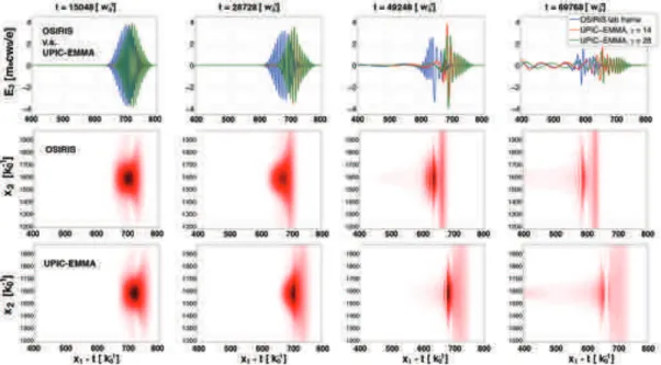
Figure 9 shows the comparison of the laser E3 fields for the three a0=4.0
cases. In the top row we show line outs of the laser at four di↵erent propaga-tion distances (times). The OSIRIS lab frame curve slips backwards. As in the other cases, the boosted frame curves line up at the front of the laser and as in the other nonlinear case di↵erences in the curves are seen in the back of the laser. In addition, for the b = 14 case we transform not only the
on-axis data, but also the o↵-on-axis data in order to compare the 2D laser profile between OSIRIS lab frame run and UPIC-EMMA boosted frame run. The OSIRIS lab frame data is shown in the middle row and the UPIC-EMMA data in the bottom row. Only a part of the the simulation box is shown. Good agreement is found in how the laser pump depletes between the two runs and in how the shape evolves. The slippage of the OSIRIS simulation results is seen.
Last, to illustrate that UPIC-EMMA is fully working in three-dimensions, we present the 3D results of UPC-EMMA using the simulation parameters in table 2 and a0=4.0. These parameters are similar to those in Ref. [2].
In figure 10 (a) and (b) we present 2D slices in the boosted frame of the plasma density and wakefield at the center of the box in the ˆ3-direction at t0 = 15335! 1
0 . As in the 2D cases, no noise from the numerical Cerenkov
instability is evident. In figure 10 (c) , the wakefield at t = 3980 !01 in the
lab frame from the OSIRIS lab frame simulation (blue) and UPIC-EMMA boosted frame simulation (red) are shown. The curves agree well but not
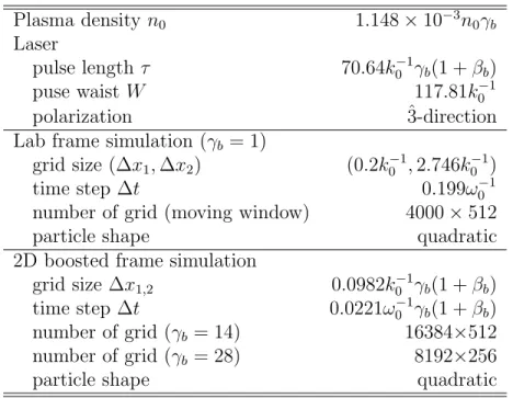
Plasma density n0 1.148⇥ 10 3n0 b
Laser
pulse length ⌧ 70.64k01 b(1 + b)
puse waist W 117.81k01
polarization ˆ3-direction
Lab frame simulation ( b = 1)
grid size ( x1, x2) (0.2k01, 2.746k01)
time step t 0.199!01
number of grid (moving window) 4000⇥ 512
particle shape quadratic
2D boosted frame simulation
grid size x1,2 0.0982k01 b(1 + b)
time step t 0.0221!01 b(1 + b)
number of grid ( b = 14) 16384⇥512
number of grid ( b = 28) 8192⇥256
particle shape quadratic
Table 1: Simulation parameters for the 2D simulations, with a0 = 0.1, 3.0, 4.0 (related
to figure 6, 7, 8, and 9). The laser frequency !0 and laser wave number k0 are used to
normalize simulation parameters, and n0= me!02/(4⇡e2).
perfectly. Note that in (c), there is no slippage because we are showing the result at a time where little slippage has occurred. Future work will involve understanding these di↵erences for these nonlinear cases.
6. Summary
In this paper, we described the rapid development of a new three di-mensional PIC code that can be used to model laser wakefield acceleration in the Lorentz boosted frames. In such simulations a plasma is drifting at relativistic speeds towards the laser, which leads to the numerical Cerenkov instability. The growth rates and unstable mode numbers of the numerical Cerenkov instability depends on the type of Maxwell field solver used. The new code, called UPIC-EMMA, uses a spectral field solver, and is fully par-allelized. It is built using the components of the UPIC Framework, which is a set of modules for building parallelized PIC codes with FFT based (spec-tral) solvers. The use of a spectral solver in which the fields are solved for in Fourier space allows for more convenient mitigation of the numerical
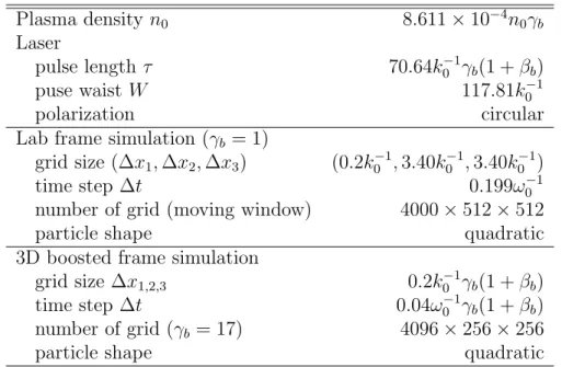
Plasma density n0 8.611⇥ 10 4n0 b
Laser
pulse length ⌧ 70.64k01 b(1 + b)
puse waist W 117.81k01
polarization circular
Lab frame simulation ( b = 1)
grid size ( x1, x2, x3) (0.2k01, 3.40k01, 3.40k01)
time step t 0.199!01
number of grid (moving window) 4000⇥ 512 ⇥ 512
particle shape quadratic
3D boosted frame simulation
grid size x1,2,3 0.2k01 b(1 + b)
time step t 0.04!01 b(1 + b)
number of grid ( b = 17) 4096⇥ 256 ⇥ 256
particle shape quadratic
Table 2: Simulation parameters for the 3D simulations (related to figure 10). The laser frequency !0and laser wave number k0are used to normalize simulation parameters, and
n0= me!20/(4⇡e2).
Cerenkov instability. The phase velocity of light in vacuum and in a plasma is always greater than the speed of light for a spectral solver. In such cases, the fastest growing modes of the numerical Cerenkov instability are due to the lowest order aliased beam mode and they reside at large values of |~k|. These modes can be easily filtered out using a “hard” low pass or “shell” filters, thereby eliminating the fast growing modes of the instability.
We presented examples of LWFA boosted frame simulations using UPIC-EMMA. Several di↵erent values of the laser amplitude were simulated ranging from a very linear regime to a nonlinear regime. For the cases shown there was no evidence of the numerical instability and good agreement was found between OSIRIS lab frame and UPIC-EMMA boosted frame simulations. The comparison showed that the wake and laser from OSIRIS lab frame simulation slipped behind the results from the boosted frame simulations as expected from numerical dispersion errors. We showed that the dispersion errors become smaller when results are transformed back the lab frame.
The results indicate that the use of a spectral code may be attractive for carrying out high fidelity LWFA simulations in boosted frames at high
self-trapping occurs in boosted frames where each macro-particle contains sig-nificant charge, studying and understanding the di↵erences between boosted frame and lab frame simulations for these and more nonlinear regimes, and using a moving cathode to simultaneously launch trailing beams into laser driven wakes or to study beam driven wakes.
This work was supported by DOE awards DE-FC02-07ER41500, de-sc0008491, DE-FG02-92ER40727, and de-sc0008316, and by NSF grants NSF PHY-0904039 and NSF PHY-0936266, and by NSFC Grant 11175102, thousand young talents program, and by FCT (Portugal), grant EXPL/FIS-PLA/0834/1012, and by the European Research Council (ERC-2010-AdG Grant 267841). Sim-ulations were carried out on the UCLA Ho↵man 2 Cluster, and Dawson 2 Cluster.
References
[1] T. Tajima, J. M. Dawson, Phys. Rev. Lett. 43, 267 (1979). [2] W. Lu, et. al., Phys. Rev. ST - Accel. Beams 10, 061301 (2007).
[3] S. F. Martins, R. A. Fonseca, W. Lu, W. B. Mori and L. O. Silva, Nat. Phys. Vol. 6, 311 (2010)
[4] D. F. Gordon, W. B. Mori, and T. M. Antonsen, IEEE Trans. Plasma Sci. 28, 1135 (2000).
[5] P. Mora and T. M. Antonsen, Phys. Plasma. 4, 217 (1997) [6] C. Huang, et. al., J. Comp. Phys. 217, 658 (2006)
[7] A. F. Lifschitz, et. al., J. Comp. Phys. 228, 1803 (2009) [8] J. -L. Vay, Phys. Rev. Lett. 98, 130405 (2007)
[9] S. F. Martins, R. A. Fonseca, L. O. Silva, W. Lu, W. B. Mori, Comp. Phys. Comm. 181, 869 (2010).
[10] J. -L. Vay, C. G. R. Geddes, E. Cormier-Michel, D. P. Grote, J. Comp. Phys. 230, 5908 (2011).
[11] C. D. Decker, W. B. Mori, Phys. Rev. Lett., Vol. 72, 490 (1994) [12] B. B. Godfrey, J. Comp. Phys. 15, 504 (1974)
[13] B. B. Godfrey, J. Comp. Phys. 19, 58 (1975) [14] K. Nagata, PhD thesis, Osaka University, 2008.
[15] P. Yu et.al, in Proc. 15th Advanced Accelerator Concepts Workshop, Austin, TX, 2012.
[16] B. B. Godfrey and J.-L. Vay, J. Comp. Phys., 248, 33-46 (2013) [17] X. Xu, et. al., Comp. Phys. Comm., Vol. 184, 2503–2514 (2013) [18] J. M. Dawson, Rev. Modern Phys., Vol. 55, No. 2, 403 (1983)
[19] K. Yee, IEEE Transactions on Antennas and Propagation, Vol. 14, 302 (1966)
[20] V. K. Decyk, Comp. Phys. Comm. 97, 87–94 (1995) [21] V. K. Decyk, Comp. Phys. Comm. 177, 95 (2007).
[22] M. Karkkainen, E. Gjonaj, T. Lau, T. Weiland, in Proceedings of the In-ternational Computational Accelerator Physics Conference, Chamonix, France, 2006, pp. 35–40.
[23] I. Haber, R. Lee, H. Klein, J. Boris, in: Proc. Sixth Conf. on Num. Sim. Plasmas, Berkeley, CA, 1973, pp. 46–48.; see also Appendix A of [J.-L. Vay, I. Haber, B. B. Godfrey, J. Comp. Phys. 243, 260–268 (2013)]. [24] C. H. Lai, T. Katsouleas, W. B. Mori, D. W. Whittum, IEEE Trans.
Plasma Phys., Vol 21, 1–8 (1993)
[25] J.-L. Vay, C. G. R. Geddes, E. Cormier-Michel, D. P. Grote, arXiv:1009.2727v2
[26] R. A. Fonseca, et al., in: P.M.A. Sloot, et al. (Eds.), ICCS, in: LNCS, Vol. 2331, 2002, pp. 342–351.
[27] F. S. Tsung, R. Narang, W. B. Mori, C. Joshi, R. A. Fonseca, L. O. Silva, Phys. Rev. Lett. 93, 185002 (2004) .
Figure 1: (a) shows the analytical expression for the µ = 0, ⌫1 =±1 mode of numerical
Cerenkov instability for the 2D spectral solver in (k1, k2) plot; (b) shows the “ring-shaped”
band-pass filter applied in the 2D spectral solver; and (c) shows the E2 energy evolutions
Figure 2: The plot shows the errors in the group velocity defined as vg 1 of the 2D EM
dispersion relation for various cases. Defining ✓ = 0 to be the laser propagating direction, this plot shows the propagation angle in ( ⇡/2, ⇡/2). If the error (vg 1) is larger than
zero, its corresponding point is in the right side of the vertical axis, and vice versa. The group velocity is calculated for the k0= 1.0 mode while we are using k0 x1= k0 x2= 0.1
Figure 3: (a) shows the intersections of the line ! = bk +!b0 and various EM dispersion
curves, while in (b) we magnified the region near the origin; (c) shows an example of the E3 spectrum of a 1D LWFA boosted frame simulation with the Yee solver. The hot spots
in (c) show where the transmitted and reflected waves are, and agrees with the prediction in (a). (d) shows the dependence of the transformed phase and group velocity of the EM waves in the plasma with b. The phase and group velocity converges quickly as b
Figure 4: UPIC-EMMA simulation setup for LWFA boosted frame simulation. The blue block is the plasma column; the green slice is the moving antenna at t = 0. The laser is launched via the moving antenna (moving together with the plasma column boundary at v = b) by initializing the appropriate curent in the green slice which has a typical
width of /2. The laser is likewise plotted for t = 0. Note when the laser is launched via the antenna, only the area within the antenna is initialized.
Figure 5: (a) is the 2D plot of the laser (polarized in x3direction) E3field at t = 13680 !01,
and (b) shows the laser E3 field transformed back from the boosted frame data. (c)–(f)
shows the comparison of on-axis E3field between OSIRIS data and UPIC-EMMA data at
Figure 6: Comparison of the on-axis E1and E3between OSIRIS lab frame simulation, and
UPIC-EMMA boosted frame simulation ( = 14, 28) at various time steps, for a0= 0.1.
x1 t is the coordinates moving together with the moving window.
Figure 7: Comparison of the on-axis E1and E3between OSIRIS lab frame simulation, and
UPIC-EMMA boosted frame simulation ( = 14, 28) at various time steps, for a0= 3.0.
Figure 8: UPIC-EMMA boosted frame simulation ( = 14, 28) for a0 = 4.0. First row
shows the 2D plots of plasma electron density (left), and the corresponding E1 for t0 =
6180 !01in the boosted frame ( = 14). The second row shows the on-axis E1comparison
between OSIRIS lab frame, and UPIC-EMMA boosted frame simulation ( = 14, 28). x1 t is the coordinates moving together with the moving window.
Figure 9: Comparison of the E3 field between OSIRIS lab frame simulation, and
UPIC-EMMA boosted frame simulation ( = 14, 28) at various time steps, for a0= 4.0. The first
row shows on-axis E3comparison between OSIRIS lab frame, and UPIC-EMMA boosted
frame ( = 14, 28). The second and third rows show the 2D comparison between the OSIRIS lab frame results and the transformed data from UPIC-EMMA boosted frame ( = 14). x1 t is the coordinates moving together with the moving window.
Figure 10: Results from 3D UPIC-EMMA boosted frame simulation ( = 17). (a) and (b) present 2D cross section plot of the plasma electron density, and E1 at t0 = 15335 !01,
while (c) shows the on-axis E1comparison at t = 3980 !01in the lab frame. x1 t is the