Error Orthogonal Models: Structure, Operations and Inference

(1)

UNIVERSIDADE DA BEIRA INTERIOR

Error orthogonal models:

Structure, Operations and Inference

Carla Maria Lopes da Silva Afonso dos Santos

Tese para obtenção do Grau de Doutor em

Matemática Aplicada

(3º ciclo de estudos)

Orientador: Prof. Doutor João Tiago Praça Nunes Mexia

Co-orientador: Prof. Doutora Célia Maria Pinto Nunes

(2)

(3)

Acknowledgements

First I would like to express my very special thanks to my supervisor, Professor João Tiago Mexia. His continuous support, encouragement, friendship and endless patience allowed me to overcome the many obstacles that came along this path.

I would also like to thank my co-supervisor Professor Célia Nunes who always supported me with kindness, encouragement and friendship and with whom I could always count despite the physical distance.

I am so fortunate to have two such wonderful persons as supervisors. It has been a very long journey and I could not have reached the goal without you two. It was an honour to work with you.

I would also like to acknowledge the huge amount of support and encouragement from my wonderful loving family. Especially to my little girl, Inês, your smile and your love light up my life and give me strength to overcome all odds.

(4)

(5)

Abstract

In this thesis, we develop the theory of Error-Orthogonal Models availing ourselves of the identity of these models and those with Commutative Orthogonal Block Structure.

Thus our treatment will rest on the algebraic structure of the models.

In our development we consider: the estimation of variance components; crossing and nesting of models; model joining, in which observations vectors obtained separately are jointly analyzed; step nesting which require much less observations than the corresponding usual models.

To broaden our treatment we also consider L Extensions of Error-Orthogonal models. In this way, we may consider interesting cases such as models otherwise balanced with different numbers of replicates for the treatments.

Last we include normality. We will be interested in obtaining sufficient statistics as well as conditions for them to be complete. We will carry out inference and consider orthogonal L extensions.

Keywords

Orthogonal block structure, commutative orthogonal block structure, error-orthogonal model, segregation, matching, binary operations, L extensions.

(6)

(7)

Resumo

Nesta tese é desenvolvida a teoria dos modelos Error-orthogonal recorrendo à identidade entre estes modelos e os modelos com estrutura ortogonal de blocos comutativos.

Desta forma, o tratamento apresentado irá assentar na estrutura algébrica dos modelos. No desenvolvimento considera-se: a estimação das componentes de variância; o cruzamento e aninhamento de modelos; a junção de modelos, na qual vectores das observações obtidos separadamente são analisados conjuntamente; aninhamento em escada, que requer muito menos observações do que os modelos correspondentes.

Para alargar o tratamento apresentado consideram-se também Extensões L de modelos

Error-orthogonal. Desta forma, poderemos considerar casos interessantes como o dos modelos com número diferente de repetições para os vários tratamentos.

Por fim, inclui-se o caso normal. Com base no pressuposto da normalidade pretende-se obter estatísticas suficientes assim como condições para que estas sejam completas. É realizada inferência e consideram-se extensões L ortogonais.

Palavras-chave

Estrutura ortogonal em blocos, estrutura ortogonal em blocos comutativos, modelo

(8)

(9)

List of Figures

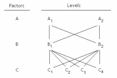
Figure 3.1 – Factors crossing ... 78

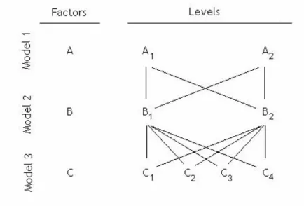
Figure 3.2 – Model Crossing... 79

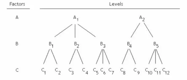
Figure 3.3 – Factors balanced nesting ... 83

Figure 3.4 – Factors unbalanced nesting ... 83

Figure 3.5 – Step nesting, with u=3,a₁=3, a₂ =2 and a₃ =4... 95

(12)

(13)

Notations and acronyms

v : Vector 0 : Null vector 1 : Vector of 1's Y : Random vector A : Matrix ⋅ : Euclidean norm X : Random matrix n

0 _: _{Null matriz of order n}

n

I : Identity matrix of order n

n

J _: _{Matrix of 1's of order n}

T

A : Transpose of the matrix A

1

A− : Inverse of the matrix A

+

A : Moore-Penrose inverse of the matrix A

B

A⊥ : Matrices A and B are pairwise orthogonal

( )

A

rank : Rank of matrix A

( )

A

det : Determinant of matrix A

( )

A

R : Range of matrix A

( )

A

Q : Ortogonal projection matrix on the range space of matrix A

( )

A

N : Nullspace of matrix A

⊗ : Kronecker matrix product

( )

V

dim : Dimension of the sub-space V

⊥

V : Orthogonal complement of V

∇

(14)

A : The algebra (CJAS) A

( )

A

dim : Dimension of the algebra (CJAS) A

( )

A

pb : Principal base of the algebra(CJAS) A

( )

M

A _: _{The algebra (CJAS) generated by}_M

Q \

M : Transition matrix between the families M and Q

⊕ : orthogonal direct sum

2 1 A

A ⊗ _: _{Kronecker product between the CJAS}A₁_andA₂

2 1 A

A ∗ _: _{Restricted Kronecker product between the CJAS}A₁_andA₂

( ) 2 1 A A

C

∗ _: _{Generalized Kronecker product between the CJAS}A₁_andA₂

2 1 A

A × _: _{Cartesian product between the CJAS}A₁_andA₂

( )

⋅

P

:

Probability

( )

X

E : Expected value of the random variable X

( )

X

V : Variance of the random variable X

( )

X,Y

COV : Covariance between random variables X and Y

( )

Y

E : Expected value of the random vector Y

( )

Y

V : Variance-covariance matrix of the random vector Y

(

X,Y

)

V : Cross-covariance matrix between the random vectors X and Y

µ

:

Mean vector

(

| ,V

)

~

X N ⋅ µ

_:

X is a normal random vector with mean vector µ and variance-covariance

matrix V

2 n

χ : Central chi-square random variable with n degrees of freedom

2 , nδ

χ

:

Chi-square random variable with n degrees of freedom and non-centrality _parameter_δ

OPM : Orthogonal projection matrix

POOPM : Pairwise orthogonal orthogonal projection matrices

(15)

JA : Jordan Algebra

CJA : Commutative Jordan Algebra

CJAS

:

Commutative Jordan Algebra of symmetric matrices

LSE

:

Least squares estimator

UMVUE : Uniformly minimum variance unbiased estimator

BLUE : Best linear unbiased estimator

UBLUE

:

Uniformly best linear unbiased estimator

OBS

:

Model with orthogonal block structure

COBS

:

Model with commutative orthogonal block structure

CCOBS

:

Model with completely commutative orthogonal block structure

EO

:

Error-orthogonal model

CEO

:

Complete error-orthogonal model

SEO

:

Error-orthogonal model with segregation

MEO

:

Error-orthogonal model with matching

EEO

:

Expanding error-orthogonal model

SCEO

:

Complete error-orthogonal model with segregation

(16)

(17)

1. Introduction

Linear models can be considered the core of linear statistical inference constituting the foundation of much of statistical practice.

Using the matrix notation we can represent a linear model by

ε β + = X

Y ,

where Y is the observations vector, X is the design matrix, ε is the errors vector and β is a vector of unknown parameters β_j, j=1,K,k, that can be all constants, all random variables or a combination of both. When some of the parameters β₀,β₁,K,β_k are considered as constants and others as random variables we have a mixed model.

Mixed models are a versatile and powerful tool for analysing data collected in experiments and, over the years, they have been applied to several areas such as biological and medical research, animal and human genetics, agriculture or industry.

For a general presentation of the theory of mixed models we can consult, for instance, Khuri et al (1998).

In our work, the mixed model

∑

= = w 0 i i i X Y β , where 0 β is fixed and w 1, ,β

β K are independent random vectors with null mean vectors

and variance-covariance matrices

w 1 c 2 w c 2 1I , ,σ I

σ K , where c_i =rank(X_i) , i=1,...,w, plays a

central part. More precisely, we will focus on those who constitute a special class within the models with Orthogonal Block Structure (OBS), this is, a particular case of the mixed models whose structure have variance-covariance matrix

∑

= = m 1 j j jQ V γ

where the Q₁,K,Q_m are known pairwise orthogonal orthogonal projection matrices such that n m 1 j j I Q =

∑

= .

OBS were introduced by J. A. Nelder , see Nelder (1965a)(1965b). These models have been intensively studied, see for instance Houtman & Speed (1983) and Mejza (1992) and

(18)

continue to play an important role in the theory of randomized block designs, see Calinski & Kageyama (2000, 2003).

Error-orthogonal models (EO), introduced by VanLeeuwen et al (1998, 1999), are models with orthogonal block structure, OBS, where the least squares estimators, LSE, for estimable vectors are uniformly best linear unbiased estimators, UBLUE, this is to say that whatever

(

γ1, ,γm

)

γ = K they are best linear unbiased estimators, BLUE. Thus, given the LSE Ψ~ and

another unbiased estimator Ψ* of an estimable vector Ψ, the difference V

( )

Ψ* −V

( )

Ψ~ of

their variance–covariance matrices is, whatever γ , a positive semi-definite matrix.

It is now convenient to recall a version of the Gauss-Markov theorem due to Zmyslony (1978) which refers that “ If the orthogonal projection matrix on the space spanned by the mean vector of the model commutes with the variance-covariance matrix, V , the LSE of estimable vectors are BLUE”. We point out that to apply this theorem it’s not necessary that

the models has orthogonal block structure and moreover that the space, Ω, spanned by

0 0

X β

µ = is the range space, R

( )

X₀ . Actually this result motivated the introduction of COBS

by Fonseca et al. (2008), as a special class of OBS in which matrix T , the orthogonal projection matrix on the space spanned by the mean vector, commutes with the matrices

m 1, ,Q

Q K . Thus, whatever γ, T and V will commute ensuring that COBS are EO.

VanLeeuwen et al (1998) showed that EO and COBS are identical classes of models. In studying EO we will favour the COBS approach which besides leading directly to UBLUE, according to Zmyslony (1978), is, as we shall see, interesting in:

- Estimating variance components;

- Building up complex models from simpler ones using, for instance, model crossing and

model nesting;

- Discussing sufficient and complete statistics once normality is assumed.

Besides this introduction this thesis comprises three more chapters.

The preliminary results chapter will be on matrices and on estimation. We start by presenting some important results on Matrix Algebra where we emphasize the Kronecker matrix product and the commutative Jordan Algebras of symmetric matrices, CJAS. These algebras are linear spaces constituted by symmetric matrices that commute and containing the squares of its matrices. Each algebra, A, has, see Seely (1971), an unique basis, the

principal basis pb

( )

A , whose elements are pairwise orthogonal orthogonal projection

matrices. These algebras play a central part when we use the COBS approach.

The results on estimation will refer to LSE and to the use of sufficient and complete statistics to obtaining good pointwise estimators. These last results will be useful in the study of the normal models.

(19)

0 0

X β

µ=

and whose variance-covariance matrix is

∑

= = w 1 i i 2 iM V σ ,

with M_i = X_iX_iT, i=1,K,w. Assuming, with R

( )

U the range space of matrix U , that

[

]

(

)

n w 1 X R X R L = ,

when matrices M K₁, ,M_w[ and T ] commute the model, as we will see, is OBS [COBS]. The first of these results is also established in VanLeeuwen et al (1998).

Next we present an independent proof of the identity of EO and COBS showing that, if LSE

are UMVUE, the OPM T commutes with the Q₁,K,Q_m.

When the model has commutative orthogonal block structure, the matrices T ,M K₁, ,M_w

will belong to a CJAS with principal basis constituted by the Q₁,K,Q_m. It may be shown that

∑

= = z 1 j j Q T , with z<m, and

∑

= = m 1 j j j , i i b Q M , i=1,K,w, so that

∑

= = m 1 j j jQ V γ

with the canonical variance components

∑

= = w 1 i 2 i j , i j b σ γ , j=1,K,m.

As we shall see, the relations between the usual and the canonical variance components will be very useful in estimating.

Next we consider building up complex models from simple ones. Namely we will consider model crossing and model nesting. In model crossing the treatments of the new model, resulting from the crossing, are all the combinations of treatments of the initial models. In model nesting each treatment of the first model nests all treatments of the other. Our

(20)

techniques for building these models will rest on binary operations on CJAS, namely the Kronecker product and restricted Kronecker product of CJAS. A third operation on CJAS, the Cartesian product, will be used in the study of model joining. Then we superimpose observation vectors and carry out joint inference. This operation also is relevant in connection with a special class of models, those derived through step nesting. This class is interesting since it leads to great economy in the number of observations.

In this third chapter we consider L extensions in which the observations vector is given by

ε + =_L_Y0

Y .

Here, Y0will be the observations vector of an EO, independent from the error vector, ε ,

and the matrix L will have linearly independent column vectors. These extension are

interesting since they include, for instance, models unbalanced in the last step.

In fourth chapter we present the normal case. When considering normality our previous treatment leads directly to sufficient statistics. As for completeness a very specific problem arises when we consider mixed models, since linear restrictions on the

z 1 ~ , , ~ _η η K or the

canonical variance components may arise and we will only have sufficient but not complete statistics.

We include in this chapter a section on inference in which we avail ourselves of the normality of the observation vectors. We also study orthogonal L extensions in which the

column vectors of matrix L are pairwise orthogonal with norm 1.

Our option of using the COBS approach, in studying the models, rests on the point that in this way the algebraic structure of the models plays a central part leading to interesting results on the estimation of variance components and on the building up of models. Moreover, as pointed above, when normality is assumed this approach leads directly to sufficient statistics. The VanLeeuwen et al (1998) definition of EO is, in our opinion, strongly connected with LSE. Now with the COBS approach the Zmyslony (1978) version of the Gauss-Markov theorem gives directly the same optimal property for the LSE as in considered in the VanLeeuwen et al (1998). So using the COBS approach we are considering both estimable vectors and variance components. It may be interesting to point out that in model build-up we obtain complex models which, when they are EO, have LSE which have optimal properties. Finally, the fifth chapter summarizes the results obtained in the preceding chapters and presents the direction in future research.

(21)

2. Preliminary results

Matrix Algebra plays an important role in many areas of Statistics. In particular in linear statistical models it’s usual to use Matrix Algebra in the presentation and verification of results, because it allows us to handle efficiently the complexity of multiple observed variables.

In this chapter we include important results on Matrix Algebra and estimation that will be needed on the remainders chapters.

We present some results in matrix theory, on topics such as orthogonal projection matrices, Moore-Penrose inverse and Kronecker matrix product, and pay special attention to commutative Jordan Algebras of symmetric matrices, CJAS, that will be used to express the algebraic structure of the models we will study.

The proofs not included in this first section can be found, for instance, in Schott (1997). The results on estimation will refer to least squares estimators, LSE, and to sufficient and complete statistics. These last results, and conjunction with the results presented for normal vectors, will be useful in the study of the normal models.

2.1. Matrices

We will restrict ourselves to real matrices, this is, matrices whose elements are all real. Let A be an n×m matrix. We will use the notation a_i_,_j to refer to the element in the i-th row and j-th column, i=1,K,n,j=1,K,m, of matrix A and we write A=

[ ]

a_i_,_j .

Computing the Euclidean vector norm on the stacked columns of an n×m matrix,

[ ]

ai,j

A= , the Euclidean norm of A is defined by

∑∑

= = = n 1 i m 1 j 2 j , i a A . (2.1.1)

When a matrix has the same number of rows as columns it is called a square matrix. An n

n× square matrix is said to be of order n.

In a square matrix the elements a_i_,_i, i=1,K,n, are called diagonal elements. If all other elements of this matrix are zero the matrix is said to be diagonal and we write,

(

a1,1, ,an,n

)

D

A= K . (2.1.2)

When a matrix is presented as a partition of several blocks (sub-matrices) we call it a blockwise matrix.

(22)

            = r 2 1 A 0 0 0 A 0 0 0 A A L M O M M L L , (2.1.3)

where 1≤r≤n, in which the off-diagonal blocks are null matrices, is called a block diagonal

matrix and we write

A=D

(

A₁K A_r

)

. (2.1.4)

2.1.1. Symmetric and orthogonal projection matrices

Definition 2.1. A square matrix, M , is said to be symmetric if M

MT = ,

this is, if the element in i -th row and j -th column equals the element in j -th row and i -th

column, for all i and j .

Definition 2.2. A square matrix, P , is said to be an orthogonal matrix if

I P P P

P T = T = ,

where I denotes the identity matrix.

The previous and the following definitions are equivalent.

Definition 2.3. If the matrix P is invertible

T 1

P

P− = ,

where P−1 is the inverse of matrix P.

Definition 2.4. Let A and B be square matrices of order n . Matrix Ais said to be similar to

matrix B, we write, A~B if there exists an invertible matrix P, of order n, such that

B P A P−1 = .

Many times we need to replace a matrix with another similar to it that is simpler, or in some way easier to deal. Being diagonal matrices the simplest matrices, we can replace the matrix by a diagonal matrix similar to it. When a matrix is similar to a diagonal matrix we say it is diagonalizable.

(23)

A symmetric matrix, M , is orthogonally diagonalizable if there is an orthogonal matrix P , whose columns are the (linear independent) eigenvectors, x₁,x₂,…,x_k, of M , such that

) , , D( MP PT = θ₁ K θ_k , (2.1.5)

where D(θ₁,K,θ_k) is the diagonal matrix whose principal elements are the eigenvalues,

k 1, ,θ

θ K , of M .

The inverse of a matrix is defined for square invertible matrices but often, in the study of Statistics, we need to use a matrix that behaves like an inverse for rectangular or singular matrices. Moore, in 1920, and Penrose, in 1955, developed a generalized inverse, for any

n

m× matrix, that possesses four properties that the inverse of a square invertible matrix has.

Given an m×n matrix A there is an unique n×m matrix A , the Moore-Penrose inverse +

of A , satisfying the conditions:

A A AA+ = , (2.1.6) + + +_AA ₌_A A , (2.1.7) + +₎ ₌_AA (AA T , (2.1.8) A A A) (A+ T = + . (2.1.9)

For any invertible square matrix A,

-1

A

A+ = . (2.1.10)

Since

( ) ( )

AT + = A+ T, if A is symmetric, A will be symmetric. + With M symmetric, we will have

(

)

    = = + + + _P _D _, _, _P M P , , D P M k 1 T k 1 T θ θ θ θ K K , (2.1.11) where     = = = ≠ = − + k , , 1 j , 0 when , 0 k , , 1 j , 0 when , j j 1 j j K K θ θ θ θ . (2.1.12)

Proposition 2.1. A matrix P is an orthogonal projection matrix (OPM) if and only if it is

(24)

Proof. Given a vector space V any vector x∈V , can be uniquely expressed as x=x₁+x₂ where x is in a subspace ₁ S⊆V and x is in the orthogonal complement, ₂ S . If P is an ⊥ orthogonal projection matrix of x onto S , Px=x₁ and Px₁ =x₁, that means that further projections to S should have no effect on Px₁. So Px=x₁=Px₁=P

( )

Px =P2x and

(

P−P2

)

x=0. Once x is arbitrary, we have P =P2, which mean that P is an idempotent matrix.

Being x₁ the orthogonal projection of x, noting that x₂ =x−x₁=

(

I−P

)

x, we have

(

I P

)

x P

x x x

0= ₁T ₂= T T − hence PT

(

I−P

)

=0 so that PT =PTP and P =PPT then P is

symmetric. Conversely, if P is a symmetric and idempotent matrix,

(

x x

)

x

(

Px P x

) (

x P P

)

x 0

P x x

x₁T ₂ = T T − ₁ = T − 2 = T − 2 = ,

hence P is an orthogonal projection matrix.

Proposition 2.2. If P is an OPM its eigenvalues will be equal to 0 or to 1.

Proof. Being P an OPM and x an eigenvector of matrix P for the eigenvalue λ, we have

( ) ( )

Px P x Px x P x P x P x 2 λ λ λ2

λ = = = = = = . Since eigenvectors are non-null vectors

(

1

)

x 0 x

x=λ2 ⇔λ −λ =

λ only occurs when λ =0 or λ =1 .

From Proposition 2.1 it follows that, if Q is an OPM then Q

Q+ = . (2.1.13)

Definition 2.5. Two orthogonal projection matrices, Q and ₁ Q , are pairwise orthogonal, ₂ we put Q₁⊥Q₂, when k k T k k 1 2Q 0 0 Q = _× = _× ,

where 0_r_×_s is the r×s null matrix.

Proposition 2.3. If Q and ₁ Q are pairwise orthogonal orthogonal projection matrices, ₂

POOPM, then Q₁ +Q₂ is an orthogonal projection matrix.

(25)

(

Q1 +Q2

)(

Q1 +Q2

)

=Q1Q1 +Q1Q2 +Q2Q1+Q2Q2 =Q1+Q2 ,

since Q and 1 Q are idempotent and pairwise orthogonal matrices, the sum of two pairwise 2

orthogonal orthogonal projection matrices is an orthogonal projection matrix.

In what follows, families of pairwise orthogonal orthogonal projection matrices, FPOOPM, will play a central part.

Moreover, see Mexia (1995), the orthogonal projection matrix on the range space of matrix X ,Ω=R

( )

X , will be

( ) ( )

_Ω ₌_Q_X ₌ _X

( )

_X _X+_X ₌_XX+

Q T T . (2.1.14)

We point out that

( )

T T

X X X

X+ = + , (2.1.15)

which reduces the problem of obtaining Moore-Penrose inverses to getting them for symmetric matrices.

2.1.2. B-matrices

These matrices are relevant in connection with least square estimator, LSE, as we shall see.

Definition 2.6. An r×s matrix C=

[ ]

c_i_,_j is a B-matrix when

       = = = =

∑

= = ,s , 1 j c c ,r , 1 i c c r 1 i i,j r 1 s 1 j i,j s 1 K K , where

∑∑

= = × = r 1 i s 1 j j , i c s r 1 c .

(26)

, c c c c J C c c c c C J s 1 j j r, s 1 s 1 j j r, s 1 s 1 j j 1, s 1 s 1 j j 1, s 1 s s 1 r 1 i s i, r 1 r 1 i i,1 r 1 r 1 i s i, r 1 r 1 i i,1 r 1 r r 1                                                       =                           =

∑

= = = = = = = = L M M L L M M L

withJ_n =1_n1T_n, where 1 is the _n n×1 vector with all components equal to 1, thus

s r J s 1 C C J r 1 = .

Proof. Since C is a B-matrix, we have

         = = = =

∑

= = = = = = = = s 1 j j , r s 1 r 1 i s , i r 1 s 1 j j , r s 1 r 1 i 1 , i r 1 s 1 j j , 1 s 1 r 1 i s , i r 1 s 1 j j , 1 s 1 r 1 i 1 , i r 1 c c c c c c c c L M M L , thus _r J_s s 1 C C J r 1 = .

We now establish the following lemma,

Lemma 2.1. We have _r J_s s 1 C C J r 1

(27)

Proof. If _r J_s s 1 C C J r 1 = we have

∑

= = = = r 1 i s , i r 1 r 1 i 1 , i r 1 _c _L _c _{as well as}

∑

= = = = s 1 j j , r s 1 s 1 j j , 1 s 1 _c _L _c _{, so}

∑∑

∑

= = = = r 1 i s 1 j j , i r 1 i j , i c s 1 c , j=1,K,s and

∑

∑∑

= = = = r 1 i s 1 j j , i s 1 j j , i c r 1 c , i=1,K,r and C is a B-matrix.

Inversely, if C is a B-matrix it is straightforward to see that the conditions of having

s r J s 1 C C J r 1 = holds.

2.1.3. Kronecker matrix products

The Kronecker matrix product is a special type of matrix multiplication without size restrictions. This product gives the possibility to obtain a composite matrix of the elements of any pair of matrices.

The Kronecker product has important applications in Statistics, namely on the representation of variance-covariance matrices. We will repeatedly use this operation which has been widely studied, see, for instance, Steeb (1991), Graham (1981) and Steeb & Hardy (2011).

Definition 2.7. Given A =[a_i,_j ], an m×n matrix, and B=[b_k,_l], an p×q matrix, the

Kronecker product between A and B , denoted by A⊗B, is defined as the mp×nq matrix

          = ⊗ B a B a B a B a B A n , m 1 , m n , 1 1,1 L M O M L .

The Kronecker product is not commutative but it satisfies the associative law, whatever matrices A , B and C , since

C B A C ) B A ( ) C B ( A ⊗ ⊗ = ⊗ ⊗ = ⊗ ⊗ . (2.1.16)

Let A and B be m×n matrices and C and D p×q matrices, we have

(

A+B

) (

⊗ C+D

)

=A⊗C+ A⊗D+ B⊗C+B⊗D , (2.1.17) which means that the Kronecker product satisfies the distributive law.

Let A be an m×n matrix and B a p×q matrix, for scalar α , we have

(28)

The next proposition, about the mixed product property, provides a very important and useful fact regarding the interchangeability of the conventional matrix product and the Kronecker product.

Proposition 2.5. Let A , B , C and D be m×n, r×s, n×p and s×t matrices, respectively. If the usual matrices products AC and BD are defined, then

BD AC D) B)(C (A⊗ ⊗ = ⊗ . Proof.

(

)(

)

                    = ⊗ ⊗ D c D c D c D c B a B a B a B a D C B A p , n 1 , n p , 1 1,1 n , m 1 , m n , 1 1,1 L M O M L L M O M L                 =

∑

= = = = n 1 k kp mk n 1 k 1 k mk n 1 k kp k 1 n 1 k 1 k k 1 BD c a BD c a BD c a BD c a L M O M L = AC⊗BD.

Proposition 2.6. For all matrices A and B ,

B A B) (A⊗ T = T ⊗ T . Proof.

(

)

T T n , m n , 1 1 , m 1,1 T n , m 1 , m n , 1 1,1 T B A B a B a B a B a B a B a B a B a B A = ⊗           =           = ⊗ L M O M L L M O M L .

Corollary 2.1. Given A and B symmetric matrices, B A B)

(A⊗ T = ⊗ ,

this is, the Kronecker product of symmetric matrices gives symmetric matrices.

Proof. Since A and B are symmetric matrices, from Proposition 2.6,

B A B A B) (A⊗ T = T ⊗ T = ⊗ .

(29)

Proposition 2.7. The Kronecker product of idempotent matrices gives idempotent matrices.

Proof. Defined the usual matrices products, with A and B idempotent, we will have from mixed product property (Proposition 2.5.),

(A⊗B)(A⊗B)=(AA)⊗(BB)= A⊗B.

From Corollary 2.1. and Proposition 2.7 it follows that, the Kronecker product of orthogonal

projection matrices gives orthogonal projection matrices. Moreover, if Q₁⊥Q₃ and

4 2 Q

Q ⊥ , with Q , ₁ Q , ₂ Q and ₃ Q OPM we will have ₄

(

Q₁ ⊗Q₂

)(

Q₃⊗Q₄

) (

= Q₁Q₃

) (

⊗ Q₂Q₄

)

=0, with 0 a null matrix, and so

(

Q1 ⊗Q2

) (

⊥ Q3⊗Q4

)

.

Proposition 2.8. Whatever matrices A and B , we have

(

_A_⊗_B

)

+ ₌_A+ _⊗_B+_. Proof. We have

(

A⊗B

)

(

A+ ⊗B+

)

(

A⊗B

)

=

(

AA+A

) (

⊗ BB+B

)

=A⊗B

and

(

_A+_⊗_B+

)

(

_A_⊗_B

)

(

_A+_⊗_B+

) (

₌ _A+_A_A+

) (

_⊗ _B+_B_B+

)

₌_A+ _⊗_B+

thus, the first and second conditions for A+ ⊗B+ to be Moore-Penrose inverse of A⊗B hold.

Once

(

)(

)

[

]

T

[

(

)

(

)

]

T

[

( ) ( )

]

T

( ) ( )

T T BB AA BB AA B A B A B A B A⊗ ⊗ + = ⊗ + ⊗ + = + ⊗ + = + ⊗ + =

( ) ( )

AA+ ⊗ BB+ =

(

A⊗B

)

(

A+ ⊗B+

)

=

(

A⊗B

)(

A⊗B

)

+

thus, also the third condition for A+ ⊗B+ to be Moore-Penrose inverse of A⊗B holds. The

fourth condition for A+ ⊗B+ to be Moore-Penrose inverse of A⊗B can be proved

analogously.

(30)

Next, with Q

( )

A [Q

( )

B ] the OPM on the range space, R

( )

A [R

( )

B ], of A [ B ], we can establish

Proposition 2.9. Whatever matrices A and B , we have

(

A B

) ( ) ( )

QA QB

Q ⊗ = ⊗ .

Proof. From (2.1.14) and Propositions 2.5 and 2.8., we have

(

A B

) (

A B

)(

A B

)

(

A B

)

(

A B

) ( ) ( )

AA BB Q

( )

A Q

( )

B

Q ⊗ = ⊗ ⊗ + = ⊗ + ⊗ + = + ⊗ + = ⊗ .

2.1.4. Jordan algebras

Jordan algebras were introduced by Pascual Jordan, in 1933, in his paper devoted to the axiomatic foundation of quantum mechanics and developed one year later in partnership with John von Neumann and Eugene Wigner, see Jordan et al (1934). Later on Seely (1970a) rediscover these structures and used them to solve problems in statistical inference and estimation area, calling them quadratic vector spaces. For priority sake we will call them Jordan Algebras. With Seely was initiated a very fruitful research line with relevant developments of linear statistical inference, see Seely (1970b, 1971, 1977) and Seely & Zyskind (1971).

Later, in Michalski & Zmyslony (1996) and (1999), the Jordan algebras have been used in hypothesis test, first for variance components and later for linear combinations of parameters in mixed linear models.

More recently the papers of Vanleuwen et al (1998, 1999) are highly interesting opening new research areas which we will pursue.

We can also quote Fonseca et al (2003, 2006, 2007, 2008, 2009), Rodrigues & Mexia (2006) and Jesus et al (2007, 2009a, 2009b).

For completeness sake, the definition of algebra is stated.

Definition 2.8. An algebra, A, is a linear space provided with a binary operation, denoted here by ∗, usually called product, that satisfies the following conditions, for all α∈IR and all x, y, z ∈A: z x y x ) z y ( x ∗ + = ∗ + ∗ z y z x z ) y x ( + ∗ = ∗ + ∗ ) y ( x y ) x ( ) y x ( ∗ = ∗ = ∗ ⋅ ⋅ α α α         

(31)

This product also enjoys the associative and commutative properties, defined below, however these properties are not necessary for a linear space to be an algebra.

Definition 2.9. If, for all x, y, z ∈A,

) z y ( x z ) y x ( ∗ ∗ = ∗ ∗ ,

the algebra A is said to be an associative algebra.

Definition 2.10. If, for all x, y ∈A,

x y y

x ∗ = ∗ ,

the algebraA is said to be a commutative algebra.

Definition 2.11. A Jordan algebra (JA) is a commutative algebra, A, whose product satisfies the Jordan identity

(

y x

)

(

x y

)

x

x2 ∗ ∗ = 2 ∗ ∗

with x2=x ∗x , for all x, y ∈A.

Definition 2.12. When the matrices of a JA commute it is called a commutative Jordan algebra, CJA.

Definition 2.13. When a CJA is constituted by symmetric matrices it is called a commutative Jordan algebra of symmetric matrices, CJAS.

In order to summarize what was previously set, we can say that a commutative Jordan algebra of symmetric matrices is a linear space constituted by symmetric matrices that commute containing the squares of their matrices.

To avoid going beyond the objectives of our study we will restrict ourselves to CJAS. For a deeper study of Jordan algebras see for instance Jacobson (1953).

Let Q =

{

Q₁,...,Q_m

}

be the principal basis of the CJAS A, pb

( )

A . Given M a matrix

belonging to a CJAS A, we have

( )

∑

∈ = = = M j j j m 1 j j jQ bQ b M C , (2.1.19) with C

( )

M =

{

j:b_j≠0

}

.

(32)

Then the Moore-Penrose inverse of M is

∑

= + + ₌ m 1 j j jQ b M , (2.1.20) where b_j+ =b_j−1 ,∀b_j ≠0 j=1,K,m, and so

( )

M C

( )

M C + =

thus, a CJAS contains the Moore-Penrose inverses of any of its matrices. With

( )

j j =RQ ∇ , j=1,K,m and

( )

j j rank Q g = , j=1,K,m,

representing by ⊕ the orthogonal direct sum of subspaces, we have

( )

_{( )}

( )

( )         = = ∇ ⊕ =

∑

∈ ∈ M C j j j M C j g M rank M r M R .

Moreover the orthogonal projection matrix on R

( )

M will be

( )

∑

∈ = M C j j Q M Q . (2.1.21)

Proposition 2.10. The orthogonal projection matrices belonging to a CJAS, A, are sums of matrices of the pb

( )

A .

Proof. Given Q , an orthogonal projection matrix belonging to A, we have

∑

= = m 1 j j jQ b Q .

Since Q is idempotent and Q₁,K,Q_m are idempotent and pairwise orthogonal,

2 m 1 j j 2 j m 1 j j jQ b Q Q b Q =

∑

=

∑

= = = ,

(33)

( )

∑

∈ = Q C j j Q Q .

Since Q =

{

Q₁,...,Q_m

}

=pb

( )

A has m matrices, A, as a linear subspace, has dimension

( )

m

dimA = . Thus there can be 2m OPM in A, as such as the distinct sums of matrices of

( )

A

pb , once each of the sums corresponds to a sub-set of m =

{

1,K,m

}

. Given C⊆ m,

( )

C Q Q C j j

∑

∈ = so that, with r

( )

C =rank

(

Q

( )

C

)

, we will have

( )

∑

∈ = C j j g C r .

We point out that we are considering the 0_n_×_n matrices as an OPM on

{ }

0n .

We also see that if, with Q∈A, we have r

( )

Q =1 then we must have Q∈Q =pb

( )

A . Namely, withJ_n =1_n1_nT, if n J n 1 Q= ,

we put Q₁=Q and say that A is a regular CJAS.

We are assuming that the matrices in A are n×n.

Definition 2.14. When a CJAS, A, contains invertible matrices we say that it is complete.

If A contains invertible matrices we must have

∑

= = m 1 j n j I Q , (2.1.22)

since we must have

∑

= = m 1 j j n

g , then the matrices in the principal basis of a complete CJAS

add up to I_n.

Let M be a matrix belonging to a CJAS, we say M is regular if and only if

( )

M n

{

1, ,n

}

C = = K . Given

∑

= = m 1 j j jQ b M , (2.1.23)

(34)

with b_j ≠0, j=1,K,m, the b , _j j=1,K,m, will be the eigenvalues of M with multiplicities g , _j j=1,K,m, so the determinant of matrix M will be

∏

= = m 1 j g j j b ) M det( (2.1.24) and

∑

= − − ₌ m 1 j j 1 j 1 Q b M .

Given the family M=

{

M₁,K,M_w

}

of matrices of A, we will have

∑

= = m 1 j j j , i i b Q M , i=1,K,w

and B=

[ ]

b_i_,_j will be the transition matrix between M and Q , M\Q . The matrices in M are linearly independent when and only when the row vectors of B are linearly independent. Since dim

( )

A =m, if w =m and the matrices M K₁, ,M_m are linearly independent the m row vectors of B will be linearly independent, thus B will be m×m and rank

( )

B =m. Then B will be invertible and with B−1=

[ ]

bl,h we will have

∑

= = m 1 h m h . l l b M Q , l=1,K,m and M=

{

M₁,K,M_w

}

will be a basis for A.

Now, the matrices of M=

{

M₁,K,M_w

}

commute if and only if they are diagonalized by

the same matrix, P . We then have o

( )

_Po M⊂V ,

with V

( )

Po the family of matrices diagonalized by P . Since o V

( )

Po is a CJAS, we see that a

family of n×n symmetric matrices is contained in a CJAS if and only if they commute. Since

the intersection of CJAS gives CJAS there will be a minimum CJAS containing M, whose

matrices commute, this will be the CJAS A

( )

M generated by M.

Namely if D is a FPOOPM, A

( )

D will have D as principal basis since the CJAS containing

D must contain the CJAS constituted by the linear combinations of the matrices.

If the M₁,K,M_w commute and are diagonalized by the orthogonal matrix P the row o vectors α₁,Kα_n of P will be eigenvectors for the matrices of o M.

(35)

Definition 2.15. Let α₁,Kα_n be the eigenvectors of matrix M . We say that exists an equivalence relation, τ , on

{

α₁,Kα_n

}

, writing α_hτ α_l , when and only when

l i T l h i T h M α α M α α = i=1,K,w,

this is, when α_h and α_l , h≠l, h,l=1,K,n, are associated to identical eigenvalues for all matrices in M .

Definition 2.16. A τequivalence class is of the first type if its vectors are associated to a non

null eigenvalue for at least one matrix in M . The number of classes of first type will be the

eigenindex of M .

Besides the first type classes there may be a second type class constituted by the

eigenvectors associated to null eigenvalues for all matrices in M .

With C K₁, ,C_m the sets of indexes of the α₁,K,α_n belonging to the first type

τequivalency classes the

∑

∈ = j C i T i i j Q α α ,j=1,K,m

constitute a FPOOPM, which will be the principal basis of a CJAS, A

( )

Q with Q =

{

Q₁,K,Q_m

}

. It is easily seen that equality in (2.1.22) holds if and only if there is no second type

τequivalency class. Thus A

( )

D is complete when and only when there is no second type

τequivalency class. Let us establish Proposition 2.11. We have A

( )

M =A

( )

Q . Proof . Since

∑

= = m 1 j j j , i i b Q

M ,i=1,K,w, with b_i_,₁,K,b_i_,_m the eigenvalues of M_i , for the vectors in the different first type τequivalency classes, i=1,K,w , we have M⊆A

( )

Q so

( )

M A

( )

Q A ⊆ as well as Q

{

Q , ,Q0

}

pb

(

( )

M

)

( )

Q m 0 1 0 0 = A ⊂A = K , thus ( )

∑

∈ = l j j 0 l Q Q D , l=1,K,m0. Moreover

∑

= = 0 m 1 l 0 l 0 l , i i b Q

M , i=1,K,w, so the α₁,K,α_n with indexes in each of the sets

( )

U

l j j C D ∈

are associated to identical eigenvalues for all matrices in M which is impossible unless all sets D

( )

l , l=1,K,m0 contain an unique index. This will imply that the matrices in Q are the possibly reordered, matrices in Q . 0

(36)

Corollary 2.2. A

( )

M is complete if and only if there is no second type τequivalency class.

Corollary 2.3. The eigenindex of M equals d

( )

M =dim

(

A

( )

M

)

Corollary 2.4. A family M of commuting symmetric matrices is a basis for A

( )

M is and only if its eigenindex equals its cardinal.

When M is a basis for A

( )

M it is a perfect family of symmetric matrices. These families were studied by Ferreira et al (2007).

From the previous results we have an important result established in Seely (1971).

Theorem 2.1. Every CJAS, , has an unique basis, the principal basis A

{

Q ,...,Q

}

pb

( )

A

Q = ₁ _m =

which is a FPOOPM. Inversely every FPOOPM is the principal basis of a CJAS.

As a parting remark we point out that, given a CJAS, A, polynomials in matrices of A

belongs to A.

2.1.5. Binary operations on CJAS

We now consider binary operations on CJAS, more precisely on its principal basis. These operations will be very useful in deriving complex models from simple ones.

The first two operations, the Kronecker product of CJAS and the restricted Kronecker product of CJAS, were introduced on Fonseca et al (2006) and will be relevant for model crossing and model nesting, respectively. The last operation, the Cartesian product of CJAS, was introduced on Fernandes et al. (2010) and will be useful in considering models obtained through joining and step nesting.

2.1.5.1. Kronecker product Proposition 2.12. Given

( )

( )( )

      = Q₁ l , ,Q_m_l l l

Q K , the principal basis of the CJAS

( )

l

A , l=1,2, the Kronecker product between A

( )

1 and A

( )

2 , A

( )

1 ⊗A

( )

2 , will be the CJAS with principal basis

( )

1 Q

( )

2

{

Q_j'

( )

1 Q_j'_'

( )

2 ;j' 1, ,m

( )

1, j' ' 1, ,m

( )

2

}

Q

(37)

Proof. Being

( )

( )( )

      l l m ,Q , l 1

Q K , the principal basis of the CJAS A

( )

l , l=1,2,

constituted by pairwise orthogonal orthogonal projection matrices, the matrices

( )

1 Q

( )

2

Q_j_′ ⊗ _j_′′ , j′=1,L,m

( )

1 , j′′=1,K,m

( )

2

are also orthogonal projection matrices because, as we saw, the Kronecker product of orthogonal projection matrices is an orthogonal projection matrix. Besides this, using the distributive law of Kronecker matrix product, we have

( )

(

)

( ) ( )

∑ ∑

∑

= ′ ′′= ′ ′′ = ′′ ′′ = ′ ′ ⊗ =         ⊗         m1 1 j 2 m 1 j j j 2 m 1 j j 1 m 1 j j 1 Q 2 Q 1 Q 2 Q

thus, the kronecker of CJAS,

( )

1 A

( )

2

A ⊗ ,

is a linear space constituted by symmetric matrices that commute.

On the other hand, being M a matrix belonging toA

( )

1 ⊗A

( )

2 , there are two matrices

( )

1

M₁∈A and M₂ ∈A

( )

2 such that M=M₁⊗M₂.

Since A

( )

1 and A

( )

2 are CJAS, M₁2∈A

( )

1 and M2₂∈A

( )

2 , thus M2∈A

( )

1 ⊗A

( )

2 , because, from Proposition 2.5, M2 =

(

M₁⊗M₂

)

2 =M₁2 ⊗M2₂. Therefore A

( )

1 ⊗A

( )

2 contains the square of their matrices, it is a CJAS.

Now, follows from the Theorem 2.1 that, if Q_j_′

( )

1 ⊗Q_j_′′

( )

2 are pairwise orthogonal orthogonal projection matrices then they constitute the principal basis of the CJAS

( )

1 A

( )

2

A ⊗ .

Given the families of symmetric matrices

( )

l

{

M

( )

l , ,M ( )

( )

l

}

( )

l

M = ₁ K _w_l ⊆A , l=1,2 (2.1.25)

and B

( )

l =

[

b_i_,_j

( )

l

]

, l=1,2 , the transition matrices between M

( )

l and Q

( )

l , M

( ) ( )

l \Q l ,

2 , 1 l= , for

( )

1 M

( )

2

{

M

( )

1 M

( )

2 ;i' 1, ,m

( )

1, i' ' 1, ,m

( )

2

}

M M= ⊗ = _i' ⊗ _i'_' = L = K (2.1.26)

and Q the transition matrix will be

( )

1 B

( )

2 B

(38)

once we order the matrices in M and Q according to the indexes

(

) ( )

( )

(

) ( )

( )

   = ′′ = ′ ′′ + − ′ = = ′′ = ′ ′′ + − ′ = 2 m , , 1 j , 1 m , , 1 j , j 2 m 1 j j 2 w , , 1 i , 1 w , , 1 i , i 2 w 1 i i K K K K .

Since the Kronecker product of matrices is associative it is easy to see that

(

2 3

) (

1 2

)

3

1 A A A A A

A ⊗ ⊗ = ⊗ ⊗ , (2.1.28)

this is, the kronecker product of CJAS is associative.

Proposition 2.13. If A₁ and A₂ are regular CJAS then A₁⊗A₂ is a regular CJAS.

Proof. If A₁ and A₂ are regular CJAS , constituted by matrices of order n

( )

1 and n

( )

2 , respectively, we have

( )

Jn( )1 ∈A1 1 n 1 and

( )

Jn( )2 ∈A2 2 n 1 . Then

( )

n( )1 ⊗

_{( )}

n( )2 =

_{( ) ( )}

Jn( ) ( )1n2 ∈A1⊗A2 2 n 1 n 1 J 2 n 1 J 1 n 1 ,

thus A1 ⊗A₂ is a regular CJAS.

Proposition 2.14. If A₁ and A₂ are complete CJAS then A₁⊗A₂ is a complete CJAS.

Proof. Being A₁ and A₂ complete CJAS, constituted by matrices of order n

( )

1 and n

( )

2 ,

respectively, we have

( )

( ) ( )1 n 1 m 1 j j 1 I Q =

∑

= ′ ′ and

( )

( ) ( )2 n 2 m 1 j j 2 I Q =

∑

= ′′ ′′ . Then

( )

( ) ( ) ( )1 n( )2 n( ) ( )1n2 n 1 m 1 j 2 m 1 j j j 1 Q 2 I I I Q ⊗ = ⊗ =

∑ ∑

= ′ ′′= ′ ′′ ,

which means that A₁⊗A₂ is a complete CJAS.

2.1.5.2. Restricted Kronecker product

Proposition 2.15. Let Q

( )

l =

{

Q₁

( )

l,K,Q_m_{( )}_l

( )

l

}

, be the principal basis of the CJAS A_l ,

2 , 1 l = . Putting

( )

n( )2 1 J 2 n 1 2

Q = , the restricted Kronecker product between A₁ and A₂,

A

(39)

( ) ( )

J ( )

{

I ( ) Q

( )

2, ,I ( ) Q ( )

( )

2

}

2 n 1 1 Q , , J 2 n 1 1 Q Q Q Q ₁ _n₂ _m₁ _n₂ _n₁ ₂ _n₁ _m₂ 2 1 _∪ ⊗ ⊗     ⊗ ⊗ = ∗ = K K

Proof. Once the Kronecker product-⊗ of OPM is an OPM, then Q_∗ =Q_∗

( )

1 ∪Q_∗

( )

2 , where

( )

1

{

Q

( )

1 Q

( )

2, ,Q ( )

( )

1 Q

( )

2

}

Q_∗ = ₁ ⊗ ₁ K _m₁ ⊗ ₁ and Q_∗

( )

2 =

{

I_n_{( )}₁ ⊗Q₂

( )

2,K,I_n_{( )}₁ ⊗Q_m_{( )}₂

( )

2

}

, will be a family of orthogonal projection matrices.

1) Given two matrices Q_i

( )

1 ⊗Q₁

( )

2 and Q_i_′

( )

1 ⊗Q₁

( )

2 belonging to Q_∗

( )

1 , we have

( )

(

Q_i 1 ⊗Q₁ 2

) ( )

(

Q_i_′ 1 ⊗Q₁

( )

2

)

=

(

Q_i

( ) ( )

1Q_i_′ 1

)

⊗

(

Q₁

( ) ( )

2Q₁ 2

)

=0.

2) Given two matrices I_n_{( )}₁ ⊗Q_j

( )

2 and I_n_{( )}₁ ⊗Q_j_′

( )

2 , j≠j′, belonging to Q_∗

( )

2 , we have

( )

(

I_n₁ ⊗Q_j 2

)

(

I_n( )₁ ⊗Q_j_′

( )

2

)

=

(

I_n( ) ( )₁ I_n₁

)

⊗

(

Q_j

( ) ( )

2 Q_j_′ 2

)

=I_n( )₁ ⊗

(

Q_j

( ) ( )

2 Q_j_′ 2

)

=0.

3) With Q_i

( )

1 ⊗Q₁

( )

2 ∈Q_∗

( )

1 and I_n_{( )}₁ ⊗Q_j

( )

2 ∈Q_∗

( )

2 , we have

( )

(

Q_i 1 ⊗Q₁2

)

(

I_n( )₁ ⊗Q_j

( )

2

)

=

(

Q_i

( )

1 I_n( )₁

)

⊗

(

Q₁

( ) ( )

2 Q_j 2

)

=0

Thus,

2 1 Q

Q ∗ will be the principal basis of the CJAS A₁∗A₂.

WhenA₁ is regular A₁∗A₂ is regular. Besides this, if A₁ is complete and A₂is regular

( )

_{( )}

( ) ( )

( )

n( )2 1 m 1 j j 1 m 1 j 2 n j J 2 n 1 1 Q J 2 n 1 1 Q _⊗       =       ⊗

∑

= = ( )

_{( )}

J ( ) I ( ) Q

( )

2 2 n 1 I_n₁ ⊗ _n₂ = _n₁ ⊗ ₁ = . (2.1.29) This result will be used later on.

If A₁ is complete and A₂ is regular and complete, A₁*A₂ is complete since

( )

( ) ( ) ( )

( )

(

)

( ) ( )

( )

∑

= = = ⊗ + ⊗ = ⊗ +       ⊗ 2 m 2 j j 1 n 1 1 n 2 m 2 j j 1 n 1 m 1 j 2 n j J I Q 2 I Q 2 I Q 2 2 n 1 1 Q _{( )}

( )

( ) ( )1 n( )2 n( ) ( )1n2 n 2 m 1 j j 1 n Q 2 I I I I ⊗ = ⊗ = =

∑

= (2.1.30)

As well as the Kronecker product, the restricted Kronecker product also satisfies the associative law. Given another CJAS, A₃, with principal basis

{

Q₁

( )

3 ,K,Q_m_{( )}₃

( )

3

}

, putting

( ) ( )

n( )3 1 J 3 n 1 3 Q = we have

(40)

(

2 3

)

(

1 2

)

3

1 A A A A A

A ∗ ∗ = ∗ ∗ , (2.1.31)

see Fonseca et al (2006).

The Kronecker product and the restricted Kronecker product can be applied jointly, for instance,

(

A1⊗A2

)

∗

(

A3⊗A4

)

would be the restricted Kronecker product between A₁ ⊗A₂ and A₃ ⊗A₄.

2.1.5.3. Generalized Kronecker product

Given two CJAS A₁ and A₂ the generalized Kronecker product between A₁ and A₂, denoted as

( ) 2 1 A A

C

∗ , will be a CJAS with principal basis

( )

{

Q

( )

1 Q

( )

2, ,Q ( )

( )

1 Q

( )

2

}

{

I ( ) Q

( )

2;h C

}

pb _n₁ _h C h h 1 m h 1 C __∪ ⊗ ∉      ⊗ ⊗ =       _∗ ∈

U

K 2 1 A A (2.1.32)

The two binary operations introduced before are special instances of

( )C∗ , where

{}

1 ⊆C⊆m2 =

{

1,K,m2

}

. Putting

( )

1_{( )} 2 1/2 A A A C C = ∗ (2.1.33)

we have the kronecker product betweenA1andA2,

( )

m2 1/2 2 1 A A

A ⊗ =

and the restricted Kronecker product betweenA1andA2,

{}

( )

1 * ₂ _1/2 1 A A A = . 2.1.5.4. Cartesian product

The Cartesian product

l 2 1 lX A A A = = × 2 1 (2.1.34)

(41)

( )

l

{

D

(

Q

( )

1 ,0 ( ) ( )

)

D

(

Q ( )

( )

1,0 ( ) ( )

)

}

{

D

(

0 ( ) ( ),Q

( )

2

)

D

(

0 ( ) ( ),Q ( )

( )

2

)

}

Q X2 ₁ _n₂ _n₂ _m₁ _n₂ _n₂ _n₁ _n₁ ₁ _n₁ _n₁ _m₂ 1 l= = × ⋅ ⋅ × ∪ × ⋅ ⋅ × K K (2.1.35) where we assume that

( )

l pb

( )

{

Q

( )

l, ,Q ( )

( )

l

}

Q = A_l = ₁ K _m_l , l=1,2

and that the matrices in A_l are n

( ) ( )

l ×nl , l=1,2. Given another CJAS, A₃, we have

(

2 3

) (

1 2

)

3 1 A A A A A

A × × = × × , (2.1.36)

thus the Cartesian product is associative.

2.2. Estimation

In this section we present important results on least squares estimators, LSE, among which we highlight a version of the Gauss-Markov theorem due to Zmyslony.

Devote special attention to the commutativity of the matrices T and V which is a sufficient condition for a linear mixed model be an error-orthogonal model.

We also present an example where we consider a balanced mixed model.

2.2.1. Least squares estimators

In what follows we are interested in models with mean vector

β

µ=E(Y)=X . (2.2.1)

Definition 2.17. A vectorβ~ is the least squares estimator, LSE, of β if it minimizes

( )

2

X Y

s β = − β .

Proposition 2.16. The vectorβ~ is the least squares estimator of β if and only if Xβ~=TY, where T is the OPM on Ω=R

( )

X , the space spanned by µ.

Proof. With V the orthogonal projection of V on the subspace _∇ ∇, and Ω⊥ the orthogonal

(42)

( )

2 2 2 2 X Y Y X Y Y X Y sβ = − β = _Ω⊥ + _Ω − β = _Ω⊥ + _Ω− β .

Since Y_Ω⊥ 2does not depend on β , s

( )

β is minimized by minimizing

2 X

Y_Ω− β , this is, since TY=Y_Ω, s

( )

β is minimized by minimizing TY−Xβ 2, where T is the OPM on

( )

X R

=

Ω , the space spanned by µ. Thus the squared distance between T and Y Xβ is zero

if and only if Xβ~=TY.

Corollary 2.5. β~=

( )

XTX+XTY is the least squares estimator of β .

Proof. As we saw, the OPM on Ω=R

( )

X , the space spanned by µ, is

( )

_XT_X _XT

X

T = + .

So the minimum of s

( )

β is attained for

( )

X X X Y

~₌ T + T

β .

Besides this

Definition 2.18. Ψ=Gβ is estimable if Ψ* =UY is a linear unbiased estimator for Ψ, for

some matrix U .

Then, for everyβ, we get

β β G

UX = ,

so that G=UX which is equivalent to GT =XTUT and, see Mexia (1990),

( ) ( )

T T X R G R ≤ . If the Y U_l * l = Ψ , l=1,2, (2.2.2)

are unbiased estimators for Ψ we have

= =

(43)

so the row vectors of U₁−U₂ will be orthogonal to the column vectors of X , thus to Ω. Let us establish

Lemma 2.2. The Ψ*_l =U_lY, l=1,2, are unbiased estimators of the same estimable vector if and only if U₁T=U₂T.

Proof. If Ψ_l* and Ψ*₂ are unbiased estimators of the same estimable vector

(

U₁−U₂

) (

T= U₁−U₂

)

X

( )

XTX +XT =0, since

(

U₁−U₂

)

X=0, and so U₁T=U₂T. Inversely, the mean vectors, of Ψ_l*, E

( )

Ψ_l* =U_lXβ =U_lTXβ , l=1,2, will be equal when U₁T=U₂T, and so the proof is complete.

The LSE of the estimable vector Ψ =Aβ will be Y U ~ A ~ ₌ ₌ 0 Ψ β , (2.2.4) with

( )

T T 0 _A_X _X _X U = + .

We now have the

Proposition 2.17. The LSE of estimable vectors of models with mean vector µ =Xβ are the

Y

M , with MT= M.

Proof. Whenever µ =Xβ we have T=Q

( )

X =X

( )

XTX +XT the OPM on R

( )

X the space

spanned by µ.

If Ψ =Gβ is estimable there is an unbiased estimator for Ψ, say M for some matrix M , Y

and its LSE will be Ψ~ =Gβ~ with β~=

( )

XTX +XT Y. So

( )

X X X Y G ~ G Y M = β = T + T thus

( )

_XT_X _XT G M= + .

(44)

Since

( )

XTX + XTX

( )

XTX +is the Moore- Penrose inverse of XTX we have,

( )

X X X X

( )

X X X M G MT= T + T T + T = . Inversely, if MT=M, we have

( )

X X X Y MXβ~ X M Y T M Y M = = T + T = .

and MY is the LSE of Ψ=Gβ with G=MX.

Corollary 2.6. If Ψ* =UY is an unbiased estimator for Ψ, the LSE for Ψ will be Ψ~ =UTY.

Proof. Since UTT =UT, it suffices to point out that Ψ~ is an unbiased estimator of Ψ of the type indicated in the thesis of Proposition 2.17.

According to Zmyslony (1978), we get the following relevant version of the Gauss-Markov theorem. Before, we present some remarks which may be significant.

Remarks:

• Ψ~ is BLUE for Ψ if and only if, whatever the unbiased linear estimator for Ψ, Ψ*,

the difference V

( )

Ψ* −V

( )

Ψ~ of their variance-covariance matrices is positive semi-definite.

• If V depends on parameters, say variance components, the condition TV=VT is

assumed to hold for all possible choices of these parameters.

Theorem 2.2. (Gauss-Markov): If the model has mean vector µ= Xβ and variance-covariance matrix V that commute with the OPM T the LSE of estimable vectors are the best linear unbiased estimators, BLUE.

Proof. According to the Corollary 2.6, given the unbiased estimator Ψ* =UY of Ψ, the LSE of Ψ will be Ψ~ =UTY. Now, with V

( )

Ψ* and V

( )

Ψ~ the variance-covariance matrices of these estimators and TC =In−T, we have, since V and T commute and TTC =TCT=0,

(45)

( )

(

) (

)

( )

C C T T C C T T C C T C T C T T C C T C T C T T C C T * U VT UT ~ V U VT UT UTVTU U VT UT TVU UT VU UTT UTVTU U VT UT VTU UT U UTVT UTVTU U T T V T T U UVU V + Ψ = + = + + + = + + + = + + = = Ψ

The thesis now follows from UTCVTCUTbeing positive semi-definite and from, according to

Lemma 2.2, getting the same LSE, UT , whatever the unbiased estimator YY U for Ψ.

Given Q =

{

Q₁,K,Q_m

}

=pb

( )

A , when T∈A we can reorder the matrices in Q to get, for m z< ,        = =

∑

= = m 1 j j j z 1 j j Q V Q T γ , (2.2.5)

when V is known up to the γ₁,K,γ_m, these will be the canonic variance components.

When the row vectors of A constitute an orthonormal basis to _j ∇_j =R

( )

Q_j , we will have     = = = = m , , 1 j , I A A m , 1 j , Q A A j g T j j j j T j K K , (2.2.6)

with g_j=rank

( )

Q_j =rank

( )

A_j =dim

( )

∇_j , j=1,K,m , see Silvey(1975). Taking

       = = = = = = = = m , , 1 j , ~ Y A Y Q S m , , 1 j , A m , , 1 j , Y A ~ 2 j 2 j 2 j j j j j j K K K η µ η η , (2.2.7) j

η will be the mean vector of

j ~ η ,

( )

j ~ E η , j=1,K,m. Moreover 0 j=

η and S has mean _j

vector E

( )

S_j =g_jγ_j, j=z+1,K,m. Thus we have the unbiased estimator

j ~ η , j=1,K,m, for the j η , j=1,K,m and j j j g S ~ ₌ γ , j=z+1,K,m . (2.2.8)

Later on we will consider the estimation of the γ_j, j=1,K,z. The estimation of the usual variance components σ₁2,K,σ_w2 may present some problem. For instance, see Khuri et al (1998), in a three factors random effects balanced model in which a first factor crosses with a

Error Orthogonal Models: Structure, Operations and Inference

UNIVERSIDADE DA BEIRA INTERIOR