www.geosci-model-dev.net/7/267/2014/ doi:10.5194/gmd-7-267-2014
© Author(s) 2014. CC Attribution 3.0 License.
Geoscientiic
Model Development
A distributed computing approach to improve the performance of
the Parallel Ocean Program (v2.1)
B. van Werkhoven1, J. Maassen2, M. Kliphuis3, H. A. Dijkstra3, S. E. Brunnabend3, M. van Meersbergen2, F. J. Seinstra2, and H. E. Bal1
1VU University Amsterdam, Amsterdam, the Netherlands 2Netherlands eScience Center, Amsterdam, the Netherlands
3Institute for Marine and Atmospheric research Utrecht, Utrecht, the Netherlands
Correspondence to:B. van Werkhoven ([email protected])
Received: 5 July 2013 – Published in Geosci. Model Dev. Discuss.: 12 September 2013 Revised: 17 December 2013 – Accepted: 2 January 2014 – Published: 7 February 2014
Abstract. The Parallel Ocean Program (POP) is used in many strongly eddying ocean circulation simulations. Ide-ally it would be desirable to be able to do thousand-year-long simulations, but the current performance of POP pro-hibits these types of simulations. In this work, using a new distributed computing approach, two methods to improve the performance of POP are presented. The first is a block-partitioning scheme for the optimization of the load balanc-ing of POP such that it can be run efficiently in a multi-platform setting. The second is the implementation of part of the POP model code on graphics processing units (GPUs). We show that the combination of both innovations also leads to a substantial performance increase when running POP si-multaneously over multiple computational platforms.
1 Introduction
Physical oceanography is currently undergoing a paradigm shift in the understanding of the processes controlling the global ocean circulation. Two factors have contributed to this shift: (i) the now about 20 yr long record of satellite data and (ii) the possibility to simulate the ocean circulation using models which include processes on the Rossby deformation radius (10–50 km). Resolving this scale captures the instabil-ity processes that lead to ocean eddies which subsequently interact and affect the large-scale ocean flow (Vallis, 2006).
The level of realism (in relation to available observa-tions) in simulating the ocean with high-resolution, strongly eddying models substantially increases compared to the
low-resolution models in which the effects of eddies are parametrized. For example, it leads to a much better simu-lation of the different oceanic boundary currents, in particu-lar the separation of the Gulf Stream in the Atlantic. Also, the degree to simulate the surface kinetic energy distribu-tion, which can be compared with satellite data, markedly improves (Smith et al., 2000; Maltrud et al., 2010).
The use of the strongly eddying models is, even on the supercomputing platforms currently available, still computa-tionally expensive, and simulations have a long turn-around time. Typical performances are from one to a few model years per 24 h using thousands of cores (Dennis, 2007). Con-sidering the fact that it takes at least 1000 yr to reach a near-statistical-equilibrium state, innovations to increase the per-formance of these models and to efficiently analyse the data from the simulations have a high priority.
Today many traditional cluster systems are equipped with graphics processing units (GPUs) because of their ability to process computationally intensive workloads at unprece-dented throughput and power efficiency rates. Existing soft-ware requires modifications such as the expression of fine-grained parallelism before it may benefit from the added pro-cessing power that GPUs offer.
However, it is currently not well known which specific parts of ocean models can benefit the most from execution on GPUs, how the existing software should be revised to ef-ficiently use GPUs, and what impact the use of GPUs will have on performance. In this paper, we aim to answer these questions.
We present two innovations to improve the performance of the Parallel Ocean Program (POP). POP is also used as the ocean component of the much used Community Earth System Model (CESM). We have applied our modifications to a standalone version of POP (v2.1). However, we have confirmed through source code inspection that all of our changes are also applicable to and fully compatible with the latest release of CESM (v1.2.0). The main issue is how to adapt POP such that it can run simultaneously (and ef-ficiently) on multiple GPU clusters. First, we address al-ternative domain decomposition schemes and hierarchical load-balancing strategies which enable multi-platform sim-ulations such that further scaling can be achieved. Second, we show how POP can be adapted to run on GPUs and study the effect of GPU usage on its performance. The source code of our modified version of POP can be obtained from https://github.com/NLeSC/eSalsa-POP/.
2 Load balancing
The model considered here is the global version of POP (Dukowicz and Smith, 1994) developed at Los Alamos Na-tional Laboratory. We consider the strongly eddying config-uration, indicated byR0.1, as used in recent high-resolution
ocean model simulations (Maltrud et al., 2010; Weijer et al., 2012). This version has a nominal horizontal resolution of 0.1◦using a 3600×2400 horizontal grid with a tripolar grid
layout, having poles in Canada and Russia. The model has 42 non-equidistantzlevels, increasing in thickness from 10 m just below the upper boundary to 250 m just above the lower boundary at 6000 m depth. In addition, bottom topography is discretized using partial bottom cells, creating a more accu-rate and smoother representation of topographic slopes.
2.1 Domain decompositions and block distributions
POP supports parallelism on distributed memory computers through the message passing interface (MPI). To distribute the computation over the processors, POP uses a three-dimensional mesh, sketched in Fig. 1a. The domain is de-composed into equal-sized rectangular blocks in the hori-zontal direction. Each block also contains several layers in the vertical direction (depth). The blocks are then distributed over the available MPI tasks, where each task receives one or more blocks. Blocks consisting only of land points may be discarded from the computation. Below we will assume that a single MPI task is assigned to a processor core (unless stated otherwise).
Each block is surrounded by a halo region (Fig. 1b) that contains a copy of the information of the neighbour-ing blocks. These halos allow the calculations on each block to be performed relatively independently of its neighbour blocks, thereby improving parallel performance. Neverthe-less, the data in the halo regions need to be updated reg-ularly. This requires a data exchange between the blocks, which leads to communication between the MPI tasks, the amount of data depending on the width of the halo, the size of the blocks, and the block distribution over the MPI tasks.
In POP, the halo width is typically set to 2. For an ex-ample block size of 60×60, the number of elements that need to be exchanged per block in every halo exchange is 4×(60×2)+4×4=496. This number may need to be multi-plied by the number of vertical levels, depending on the data structure on which the halo exchange is performed. Some data structures, like the horizontal velocity, store a value for every grid point at every depth level. As a result, a 3-D halo exchange is required that exchanges elements from every depth level. Others data structures, such as surface pressure, only consist of a single level. There, a 2-D halo exchange is sufficient.
For neighbouring blocks that are assigned to the same MPI task, the data exchange is implemented by an internal copy and no MPI communication is required. Also, no data need to be exchanged with (or between) land elements. Therefore, the amount of data that needs to be communicated between MPI tasks depends heavily on the way the blocks are dis-tributed over the MPI tasks.
2.2 Existing block-partitioning schemes
POP currently supports three algorithms for distributing the blocks over the available MPI tasks, Cartesian, rake (Mar-quet and Dekeyser, 1998), and space-filling curve (Dennis, 2007). The Cartesian algorithm starts by organizing the tasks in a two-dimensional grid. Next, the blocks are assigned to these tasks according to their position in the domain. If the number of MPI tasks does not divide the number of blocks evenly in either dimension, some tasks may receive more blocks than others. In addition, some tasks may be left with less work (or even no work) if one or more blocks assigned to it only contain land. As shown in Dennis (2007), load im-balance between tasks can significantly degrade the perfor-mance of high-resolution ocean simulations.
(a) (b)
Fig. 1. (a)Sketch of the block-wise subdivision of the domain in POP.(b)The halo regions of a block; image from Smith et al. (2010).
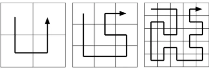
Fig. 2.Examples of the space-filling-curve load-balancing algo-rithm, with the Hilbert (left panel), meandering Peano (middle panel), and Cinco (right panel) curves; image from Dennis (2007).
This process is repeated for all tasks in the row. The pro-cess is repeated for all columns of the task grid. As described in Smith et al. (2010), the algorithm “can be visualized as a rake passing over each node and dragging excess work into the next available hole”. In an attempt to keep neighbouring blocks close together, constraints are placed on block move-ments that prevent blocks from moving too far from their di-rect neighbours. Unfortunately, there are instances where the rake algorithm actually results in a worse load balance where blocks get raked into a corner. As a result Dennis (2007) states that “we do not consider the current implementation of the rake algorithm. . . sufficiently robust.”
The space-filling-curve algorithm described in Dennis (2007) uses a combination of Hilbert, meandering Peano, and Cinco curves to partition the blocks (Fig. 2). Conceptually, it draws a single line that visits each of the blocks exactly once. It then splits this line into equal-sized segments, each segment visiting the same number of blocks. Due to the way the line is drawn, the blocks in each segment are also contin-uous in the two-dimensional domain. This solution degrades slightly when the land-only blocks are discarded, which in-troduces “cuts” in the curve. Nevertheless, the space-filling-curve algorithm significantly improves the load balance be-tween MPI tasks. A limitation of this approach is that each of the space-filling curves can only partition domains of a spe-cific size. For example, a domainP×P can be partitioned by
a Hilbert curve ifP =2n, or by a meandering Peano curve if
P =3m, wherenandmare integers. By using combinations of different curves, the set of supported problem sizes can be extended.
2.3 Hierarchical block partitioning
None of the load-balancing algorithms described in the pre-vious section takes into account the inherent hierarchical na-ture of modern computing hardware. This typically consists of multiple cores per processor, multiple processors per node, multiple nodes per cluster, and even the availability of mul-tiple clusters for a numerical simulation. The communica-tion performance drops as we go up in the hierarchy. The cores in a processor share cache memory and can therefore communicate almost instantaneously, while communication between processors has to go through main memory, which is much slower. Communication between processors on dif-ferent nodes must go through an external network, which is orders of magnitude slower, and communication between clusters in different locations is again orders of magnitude slower. Therefore, simply balancing the load for the individ-ual processors (or cores) is not sufficient. Instead, a hierar-chical load-balancing scheme must be used that takes both processor load and the communication hierarchy of the target machine into account. We suggest using a similar approach to the one used in Zoltan (Zoltan User Guide, 2013; Teresco et al., 2005). However, where Zoltan supportsdynamic load balancing(where the work distribution may change during the application’s lifetime), we compute a singlestatic solu-tionbefore the application is started.
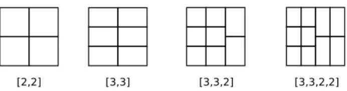
[2,2] [3,3] [3,3,2] [3,3,2,2]
Fig. 3.Example subdivisions of a square into 4,6,8, and 10 rectan-gular sections.
then partitioned into 16 pieces, which are further divided into 8 pieces. The sequence of partitionings relates directly to the hierarchy that is present in the computational platform. For example, the 2:16:8 partitioning can be used for an exper-iment on two clusters, each containing 16 nodes of 8 cores.
Once the user has specified the desired partitioning, the al-gorithm proceeds by repeatedly splitting the available blocks intoN (preferably equal-sized) subsets. We try to partition the domain in such a way that the shape of each of the sub-sets is as close to a square as possible. This will reduce the amount of communication out of each subset in relation to the amount of work inside each subset.
When splitting a domain, multiple solutions may be avail-able which are equivalent from a load-balancing perspective. However, the amount of communication required between subsets may vary between these solutions due to assignment of blocks to MPI tasks and the location of land-only blocks. Our algorithm therefore compares these solutions and selects the one which generates the least communication between subsets.
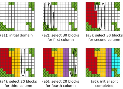
To explain our algorithm in more detail, we use the sim-plified example domain shown in the upper left panel (a1) of Fig. 4. This example domain contains 1200×1000 grid elements. It is divided into blocks of 100×100, resulting in 12×10 blocks, of which 20 are land-only blocks. To divide this domain into 10 subsets, the algorithm starts by comput-ing the required number of blocks per subset. The 100 non-land blocks must be divided into 10 subsets, resulting in 10 blocks per subset. Next, the algorithm tries to arrange the desired number of subsets in a (roughly) rectangular grid. The dimensions of this grid, consisting ofN subsets, is de-termined as follows:
f:= floor(sqrt(N)); c:= ceiling(sqrt(N))
if (f = c) we have found a square grid of [f x f] if (f*c = N) we have found a rectangular grid of [f x c] if (N < f*c) we have found a rectangular grid of [f x c]
- (f*c-N)
if (N > f*c) we have found a square grid of [c x c] - (c*c-N)
In the first two cases of the algorithm shown above, a square or rectangular decomposition is available contain-ing exactlyN subsets. In the last two cases, the decompo-sition contains (f∗c−N) or (c∗c−N) subsets too many respectively. To correct this, we repeatedly remove a single
subset from each row until the desired number of subsets is reached. Figure 3 shows four example subdivisions, for val-ues ofN=4,6,8, and 10, that correspond to each of these four cases. For our example domain we will use the rightmost subdivision in Fig. 3 for N=10 named [3,3,2,2], which represents the number of blocks in each column.
Next, we compute the required number of blocks per col-umn using the average number of blocks per subset and the selected subdivision. For our example, we will use the
[3,3,2,2] subdivision as in Fig. 3 and the 10 blocks per subset average, which will result in columns containing
[30,30,20,20] blocks. We then split the domain into sub-sets by traversing the blocks in a vertical zigzag fashion and selecting all non-land blocks until the desired number of blocks for that column in reached. It should be noted that the partitioning scheme is not a flood-fill type of algorithm, which may skip over isolated points; instead, our partition-ing scheme simply skips over any land points encountered while scanning in a certain direction, and continues scanning in a zigzag fashion until the required number of ocean (i.e. non-land) points have been selected.
The panels (a2–a6) in Fig. 4 show how the example do-main is split into the four columns. We subsequently split each of the columns in a horizontal zigzag fashion into the desired number of subsets for that column. Panels b1–b5 of Fig. 4 show an example for the first column, which needs to be split into 3 subsets of 10 blocks. A similar subdivision is applied to the other columns. The final block distribution for the example domain is shown in Fig. 4c.
As explained above, the subdivision shown in panel (c) of Fig. 4 is only one out of a series of options. Several per-mutations of the [3,3,2,2] subdivision can be created that are equivalent from a load-balancing perspective but require a different amount of communication. In addition, the sub-division can also be rotated, thereby initially dividing the domain row-wise instead of column-wise. Finally, when se-lecting the blocks in a zigzag fashion (as shown in Fig. 4), a choice can be made as to which position to start the selec-tion from: top or bottom, or left or right. In our algorithm we simply compute all unique permutations of the subdivision in all possible rotations, with all possible starting points. We then select the solution with the lowest average communi-cation per subset. If multiple equivalent solutions exist, we select the one with the lowest maximum communication per subset. Table 1 shows the best scoring results for all permuta-tions of the[3,3,2,2]subdivision. All solutions use the same number of blocks per task, but the amount of communication varies per solution. Once a domain has been split into the de-sired number of subsets, the algorithm is repeated for each of these subsets for the next split.
2.4 Hierarchical partitioning of tripole grids
(a1): initial domain (a2): select 30 blocks for ✁rst column
(a3): select 30 blocks for second column
(a4): select 20 blocks for third column
(a5): select 20 blocks for fourth column
(a6): initial split completed
(b1): ✁rst
column
(b2): select 10 blocks
for ✁rst
set
(b3): select 10 blocks for second
set
(b4): select 10 blocks for third
set
(b5): ✁rst
column completed
(c): ✁nal result
Step 1: Split domain column wise
Step 2: Split column selections row-wise (only ✁rst column selection is shown)
Fig. 4.Description of the hierarchical load-balancing scheme for an example of 12×10 blocks, of which 20 are land-only blocks, as shown
in panel(a1). The initial column-wise split is shown in panels(a2)–(a6), the next row wise split in the panels(b1)–(b5), and the final results
is shown in panel(c).
replaced with two poles located (on land) in Canada and Rus-sia, needs special attention. Note that tripolar grids are fre-quently used in ocean models because the grid spacing in the Arctic is much more uniform and the cell aspect ratios are closer to 1 when compared to traditional latitude–longitude (dipole) grids (Smith et al., 2010). In this case, additional communication is required for the blocks located on the line between these poles, as explained in Smith et al. (2010). These blocks are located on the upper boundary of the grid, as shown in Fig. 5a. To support a tripolar grid layout in our
Fig. 5. (a)A subdivision of the topography into 60×40 blocks. The two tripoles are depicted by the red dots on the upper boundary. Note that
the leftmost and rightmost dots represent the same tripole; the tripole communication is (partially) shown by the arrows.(b)A remapping of
the grid that moves an area of 30×7 blocks. The original tripole boundary is shown as a red line.
Fig. 6.An example of POP running without the MPI wrapper on a single cluster (left panel) and with the MPI wrapper on a multi-cluster (right panel).
Table 1.Permutations of the [3,3,2,2] example distribution show-ing the number of assigned blocks and the communication per task in grid points per level. The entries are sorted by average communi-cation per task. The topmost entry provides the best solution.
permutation blocks communication per task
per task (min/avg/max)
(3,3,2,2) 10 1440/2186/2888
(2,3,3,2) 10 1244/2187/2888
(2,2,3,3) 10 1240/2188/3100
(2,3,2,3) 10 1240/2188/3300
(3,2,2,3) 10 1240/2229/3720
(3,2,3,2) 10 1440/2265/2876
the grid before we start the partitioning (Fig. 5b). By sim-ply moving blocks from one side of the grid to the other, we enable our partitioning algorithm to optimize the tripole communication. Note that this remapping is only performed on the grid used in our partitioning algorithm. No change to POP is required, as POP only uses the result of the partition-ing in which the original block numberpartition-ing is maintained.
3 Results: load balancing
In this section we will compare the performance of our hier-archical algorithm to the Cartesian, rake, and space-filling-curve block-partitioning schemes. In our experiments we carry out a 10-day simulation with theR0.1version of POP, as
3.1 Hardware
The Huygens (http://www.surfsara.nl) is an IBM pSeries 575, a clustered SMP (symmetric multiprocessing) system. Each node contains 16 dual-core IBM Power 6 processors running at 4.7 GHz, resulting in 32 cores per node. As the cores support simultaneous multi-threading (SMT), every node appears to have 64 CPUs. Most applications will per-form better by using 64 MPI tasks per node (two MPI tasks per processor core). Per node, 128 GB of memory is avail-able (4 GB per core). The nodes are connected using 8×
(4×DDR) InfiniBand, resulting in a 160 Gbit s−1inter-node bandwidth.
The DAS-4 (http://www.cs.vu.nl/das4) is a six-cluster, wiarea distributed system. DAS-4 is heterogeneous in de-sign, but in this experiment we will use dual quad-core com-pute nodes containing Intel E5620 CPUs running at 2.4 GHz, resulting in eight cores per node. The nodes contain 24 GB of memory (3 GB per core). Nodes are connected using QDR InfiniBand, resulting in a 20 Gbit s−1 bandwidth. We use DAS-4 in a single-cluster and two-cluster experiment. In the two-cluster experiment, the clusters are connected using a in-ternet link with a maximum bandwidth of 1 Gbit s−1. The av-erage round-trip time between clusters is 2.6 ms. As the link is shared with other users, the available bandwidth and round trip latency may vary over time.
3.2 Using MPI for multiple clusters
For POP to run on multiple clusters, an MPI implementation is required that is capable of communicating both within and between clusters. This is far from trivial, as clusters are often protected by a firewall that disallows any incoming commu-nication into the cluster. Also, it is common for the compute nodes to be configured such that they can only communicate with the cluster frontend, but not directly with the outside world, as explained in Maassen and Bal (2007). To solve this problem, we created wrapper code that is capable of inter-cepting the MPI calls in POP. For each intercepted call, the MPI wrapper decides whether it should be forwarded to the local MPI implementation or whether it should be sent to another cluster. To use the MPI wrapper code, POP needs to be recompiled using a different MPI library; however, no changes to the POP code itself are required.
To communicate between clusters, one or more support processes, so-called hubs, are used. Each hub typically runs on the cluster frontend, and serves as a gateway to the other clusters. If necessary, multiple hubs can be connected to-gether to circumvent communication restrictions caused by firewalls. In Fig. 6, the left panel shows a traditional POP run on a single machine, while the right image illustrates how a hub is used in DAS-4 to connect two clusters together. Only a single hub is needed, as all compute nodes in DAS-4 can communicate with all head nodes, even those of other
0 50 100 150 200
cartesian 225x150 rake 60x60 sfc 60x60 hierarchical 60x60
modeldays/day
Huygens (4x64) Single Cluster DAS4 (32x8) Two Cluster DAS4 (2x16x8)
118
138 145 146
99
144
153 155
89
80
91
142
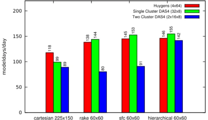
Fig. 7. Performance comparison of POP using Cartesian, rake, space-filling curve, and hierarchical block-partitioning schemes on three different hardware configurations, each using 256 MPI tasks.
clusters. However, compute nodes cannot directly communi-cate with compute nodes in other clusters.
3.3 Performance
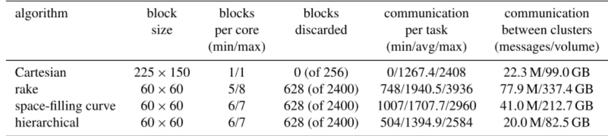
Table 2 shows the configurations of the partitioning schemes. For each experiment we use 256 MPI tasks. The Cartesian distribution uses a 225×150 block size, resulting in exactly one block per MPI task (no land blocks are discarded). Both rake and the space-filling curve use a block size of 60×60 and discard 628 of 2400 blocks (i.e. 26 %). The table also shows the minimum, average, and maximum communica-tion per MPI task, as well as the amount of traffic gener-ated between the clusters for the two-cluster experiment. We will discuss these below. As can be seen from Table 2, the hierarchical domain distribution significantly decreases the amount of traffic between the clusters compared to rake and the space-filling curve. As a result, the performance overhead of using two clusters is limited.
Table 2.Configuration of the Cartesian, rake, and space-filling curve, and hierarchical distributions.
algorithm block blocks blocks communication communication
size per core discarded per task between clusters
(min/max) (min/avg/max) (messages/volume)
Cartesian 225×150 1/1 0 (of 256) 0/1267.4/2408 22.3 M/99.0 GB
rake 60×60 5/8 628 (of 2400) 748/1940.5/3936 77.9 M/337.4 GB
space-filling curve 60×60 6/7 628 (of 2400) 1007/1707.7/2960 41.0 M/212.7 GB
hierarchical 60×60 6/7 628 (of 2400) 504/1394.9/2584 20.0 M/82.5 GB
Table 3.Speed-up on DAS-4 for one- and two-cluster configura-tions using a hierarchical domain distribution.
configuration performance speed-up
(modeldays day−1)
1 cluster, 16 nodes 82 1.0
1 cluster, 32 nodes 155 1.9
2 clusters, 16 nodes each 142 1.7
Although rake and the space-filling curve both decrease the amount of work per MPI task, they also significantly increase the amount of communication between tasks. On supercomputers, where POP is traditionally run, this prob-lem is mitigated by high-speed network interconnects, but in a multi-cluster environment, the internet link between clus-ters becomes a bottleneck. In Table 2, the column “commu-nication between clusters” clearly shows that compared to Cartesian, rake causes an increase of 3.4 times in the commu-nication between clusters. The increase caused by the space-filling curve is smaller, a factor of 2.1, but still significant.
The hierarchical scheme performs slightly better than the space-filling curve scheme on Huygens and single-cluster DAS-4 (Fig. 7). This is to be expected, as the communica-tion overhead is small on these systems due to the fast local network interconnects. On two-cluster DAS-4, however, the hierarchical domain distribution provides a significant per-formance improvement over the existing algorithms. When running on two clusters, the performance drop compared to a single-cluster run is only 8 % for the hierarchical domain distribution, compared to 10 % for Cartesian, 41 % for the space-filling curve, and 44 % for rake.
Table 3 shows the speed-up on DAS-4 compared to a 16-node run on a single cluster. The speed-up on 32 16-nodes on a single cluster is, with a factor of about 1.9, almost perfect. Although the speed-up on two-clusters (of 16 nodes each) is slightly lower, about a factor of 1.7, the performance gain compared to a single cluster is still significant. These results clearly demonstrate that using multiple clusters can be bene-ficial, especially to increase the number of machines beyond the size of a single cluster.
4 Execution on GPUs
This section discusses the main challenges that exist when moving parts of the computation in POP to a GPU. We use the CUDA programming model (Nvidia, 2013) in or-der to have fine-grained control over our GPU implemen-tation and to be able to explain and improve performance results. Many different software tools, libraries, (directive-based) parallelization tools, and compilers aim to assist in the development of GPU code. However, it is our goal to gain a deep understanding of the performance behaviour of POP, which requires more control over the implementation and in particular how data are transferred between the host mem-ory and GPU device memmem-ory. We are currently not aware of the capability to implement GPU kernels that overlap GPU computation with CPU–GPU communication in any of the existing directive-based parallelization tools for GPUs. How-ever, if this were possible, it would require a collection of directives similar to the collection of calls to the CUDA run-time that are currently responsible for achieving this overlap-ping behaviour. While directive-based parallelization tools do leave the kernel code in the same language as the original, understanding the underlying architecture is still required in order to modify that parallelized code and assess its correct-ness. In the following sections, we use CUDA terminology (Nvidia, 2013), although our methods could just as easily ap-ply to OpenCL (Khronos Group, 2013).
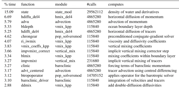
Table 4.List of the most compute-intensive functions in POP, covering 76.48 % of the total computation time. The reported time does not include time spent in functions called by this function.
% time function module #calls computes
15.09 state state_mod 29562112 density of water and derivatives
6.69 hdiffu_del4 hmix_del4 4865280 horizontal diffusion of momentum
5.79 advu advection 4865280 advection of momentum
5.33 bldepth vmix_kpp 115840 ocean boundary layer depth
5.25 hdifft_del4 hmix_del4 4865280 horizontal diffusion of tracers
4.62 chrongear pop_solversmod 115840 preconditioned conjugate-gradient solver
4.07 ri_iwmix vmix_kpp 115840 viscosity and diffusivity coefficients
3.83 vmix_coeffs_kpp vmix_kpp 115840 vertical mixing coefficients
3.66 impvmixt_correct vertical_mix 115840 implicit vertical mixing corrector step
3.34 blmix vmix_kpp 115840 mixing coefficients within boundary layer
3.27 impvmixt vertical_mix 231680 implicit vertical mixing of tracers
3.27 clinic baroclinic 4865280 forcing terms of baroclinic momentum
3.17 advt_centered advection 4865280 tracer advection using centred differencing
3.12 btropoperator pop_solversmod 14705152 applies operator for the barotropic solver
3.10 baroclinic_driver baroclinic 115840 integration of velocities and tracers
2.88 ddmix vmix_kpp 115840 add double-diffusion diffusivities
To overlap GPU communication and computation we need fine-grained control over how data are transferred to the GPU. There are several alternative techniques for moving data between host and device using the CUDA programming model. The most commonly used approach is to simply use explicit memory copy statementsto transfer large blocks of memory to and from the GPU.
Alternatively,CUDA streamsmay be used to separate the computation into distinct streams that may execute in par-allel. This way, communication from one stream can be overlapped with computation and communication in other streams. GPUs with 2 copy engines, such as Nvidia’s Tesla K20, can use the PCIe bus in full duplex with explicit mem-ory copies in different streams. This way, communication and computation from different streams can be fully over-lapped.
Finally, the mapped memory approach uses no explicit copies, but maps part of the host memory into device mem-ory space. Whether this approach is feasible depends on the memory access pattern of the kernel. Typically, mapped memory can only be used efficiently if each input and output element is read or written only once by the GPU function, calledkernel. Although this approach results in very clean host code, requiring no explicit copy statements, it requires complex kernel implementations with intricate memory ac-cess patterns to ensure high performance.
4.1 Targets for GPU implementation
To determine which part of POP to port to the GPU, we must first get an impression of where the most time is spent. It is well known that the three-dimensional baroclinic solver is the most computationally intensive part of POP (Kerbyson and Jones, 2005; Worley and Levesque, 2003). We therefore
limit ourselves to analysing the performance of the baroclinic solver.
Table 4 gives an overview of the most time-consuming functions in POP. These profiling results of are obtained from one month of simulation using theR0.1 version (see
begin-ning of Sect. 2) on the DAS-4 cluster (described in Sect. 2). For this experiment we have used a Cartesian distribution with blocks of size 255×300 and 8 processes per node on 16 nodes.
Table 4 lists the percentage of the total execution time spent in this function, not including subfunctions. All functions in Table 4, except those from the module pop solversmod, belong to the baroclinic solver. Our profiling re-sults indicate that the baroclinic solver does not contain any true computational hotspots; that is, no individual function consumes a major part of the computation time.
However, the density computations from the equation of state are requested by several different parts both within the baroclinic solver and at the end of each time step. The com-putation of water densities is required so frequently by the model that their computation time consumes 15.09 % of the total execution time on average.
It is well known that kernel-level optimizations focused on increasing computation throughput are generally not worth-while when memory bandwidth is the primary factor in lim-iting performance (Ryoo et al., 2008). A frequently used tool for performance analysis on multi- and many-core hard-ware using the Roofline model (Williams et al., 2009) is thearithmetic intensity. For example, the Nvidia Tesla K20 GPU has a theoretical peak performance of 1173 GFLOP s−1 for double precision and a theoretical peak global mem-ory bandwidth of 208 GB s−1. However, in practice the achieved memory bandwidth is (roughly) 160 GB s−1, as re-ported by the bandwidthTest tool in the Nvidia CUDA SDK. A rough estimation tells us that an arithmetic intensity of at least 7.3 FLOP byte−1 is required for the kernel to be-come compute-bound. Thus, if the arithmetic intensity is less than 7.3 FLOP byte−1, then we know the kernel is memory-bandwidth-bound when executed on the K20.
The arithmetic intensity of the state() function is computed as follows. Although POP supports various implementations for the equation of state, we focus on the 25-term equation of state (McDougall et al., 2003) because it is the most com-monly used implementation. The state() function requires the temperature and salinity tracers as inputs as well as 25 coef-ficients, of which 6 depend on the water pressure and the rest are constant. The state() function outputs the density of wa-ter and optionally also outputs the derivatives of the wawa-ter density with respect to temperature and salinity. When only the density of water is computed, state() performs 40 float-ing point operations per grid point with an arithmetic inten-sity of 2.5 FLOP byte−1, assuming that all 25 coefficients can be stored in on-chip caches and can be fully reused. When all outputs are requested, 89 floating point operations are executed per grid point, resulting in an arithmetic intensity of 5.56 FLOP byte−1. With an arithmetic intensity of either 2.5 or 5.56, the state() kernel is memory bandwidth-bound. Therefore, we focus on optimizing the time spent on com-munication between host and device rather than kernel-level optimizations.
4.2 Efficient integration of GPU code
We now describe how POP should be revised to efficiently use GPUs. For our discussion, we focus on three functions in POP state(), buoydiff(), and ddmix(). Due to a lack in GPU performance models that consider asynchronous PCIe transfers, it is currently impossible to predict what kind of implementation will be the most efficient. For each function we have therefore implemented three different versions that we callExplicit,Implicit, andStreams. We first describe the three versions in general and then discuss the specific im-plementations for state(), buoydiff(), and ddmix() in detail. Figure 8 provides a schematic overview of the three different implementations with regard to the way GPU computation (shown in green) and CPU–GPU communication (shown in blue) could be overlapped.
-Explicit implementation (uses explicit copy statements)
CPU-GPU Comm.
GPU Computation
-Implicit implementation (uses device-mapped host memory)
CPU-GPU Comm.
GPU Computation
-Streams implementation (uses CUDA Streams and explicit copy statements)
CPU-GPU Comm.
GPU Computation
Fig. 8.Schematic of the three different implementations –Explicit,
Implicit, andStreams– that shows the potential overlap between
computation and communication.
0 5 10 15 20 25 30
state buoydiff ddmix
Time (ms)
Explicit Implicit Streams
12
17
25
8
23 23
9
12
17
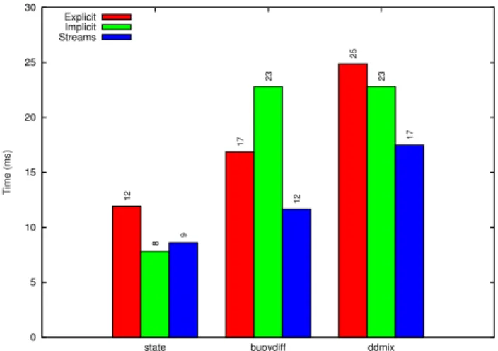
Fig. 9.Performance results for the three POP functions on a GPU with three different implementations as obtained on the Tesla K20
GPU with a 229×304 block size.
one stream for each vertical level and uses explicit copy state-ments to copy the corresponding vertical level of the input and output variables to and from the GPU. If the computa-tion of one vertical level requires input from multiple verti-cal levels, CUDA events are used to delay the computation until all inputs have been moved to the device and vice versa. The kernel used inStreamsis similar to the kernel used in Explicitexcept for the fact that the kernel only computes the grid points of one vertical level.
The three different implementations are very different in terms of code and the effort to create them. All three imple-mentations use very distinctive host codes as well as mod-ified GPU kernels. For example, the Implicit implementa-tion barely requires any host code, whereas theStreams im-plementation requires multiple loops of memory copy oper-ations and kernel invocoper-ations with advancing offsets. Note that, except for the differences described here, the kernels do not contain any architecture-specific optimizations.
While the state() function computes the density of water at a certain vertical levelk, the function is mostly used di-rectly surrounded by a loop over all vertical levels. These code blocks can safely be replaced by a call to a single func-tion that directly computes the water densities for all verti-cal levels. OurExplicitimplementation uses explicit copies to move the three-dimensional grid of tracer values between host and device and creates one thread for each horizontal grid point, which computes all outputs in the vertical direc-tion. However, this approach is unable to overlap communi-cation to and from the device with GPU computation. It is possible to also parallelize the computation of different ver-tical levels using CUDA streams. OurStreams implementa-tion ensures that GPU computaimplementa-tion can be overlapped with GPU communication of different vertical levels and thus al-leviates the PCIe bus bottleneck to a large extent. Because of the simple access pattern in state(), where each input and output element is read or written only once, it is also a good candidate for the highly parallelImplicitimplementation.
More complex uses of the equation of state are found within the computation of the vertical mixing coefficients for the KPP mixing scheme (Large et al., 1994), in particular in the computation of buoyancy differences (buoydiff) and double-diffusion diffusivities (ddmix). In POP the vertical mixing coefficients are sequentially computed for all verti-cal levels. The computation of buoyancy differences at level
krequires the density of both the surface level and levelk−1 displaced to levelk, as well as the water density at levelk. These values can be computed for each level in parallel as long as all the data are present on the GPU. Overlapping data movement from the host to the GPU with GPU computation and data movement from the GPU to host becomes signifi-cantly more difficult, because the tracers for levels 1,k−1, andkneed to be present on the GPU to compute the buoy-ancy differences at levelk. TheStreamsimplementation first schedules memory copies to the GPU for all vertical levels in concurrent streams and then invokes GPU kernel launches
for all levels. However, before the execution of the kernel in streamkcan start, the memory copies in stream 1,k−1, andkneed to be complete. The kernel executing in stream
k outputs to different vertical levels for different variables. Therefore, some of the memory copies from device to host in stream k have to wait for the kernel in stream k−1 to complete. We use the CUDA event management functions to guarantee that no computations or memory transfers start prematurely.
In the ddmix function, the computation of diffusivities at levelkrequires the derivatives of density with respect to tem-perature and salinity at levelk andk−1; that is, the com-putation of levelk reuses the derivatives that were used to compute level k−1. At a first glance, it would seem that the computation of all vertical levels cannot be parallelized. The sequential approach prevents these values having to be recomputed, but inhibits the ability to overlap communica-tion and computacommunica-tion of different vertical levels. Therefore, our implementation also parallelizes the computation in the vertical dimension by introducing double work. The cost of computing the derivatives twice is significantly less than the inability to overlap computation and communication. Simi-larly to the buoyancy differences computation, the kernel ex-ecuting in streamkrequires the memory copies of streamk
andk−1 to be complete. Again, CUDA event management functions are used to guarantee that no data are copied from the GPU back to the host before GPU computations have fin-ished.
5 Performance of POP on GPUs
In this section, we will describe the performance of theR0.1
version of POP on a single cluster and on multiple GPU clusters. In the first subsection below, we focus on the per-formance impact on individual POP subroutines when using a GPU. In the second subsection, we address the performance of the whole POP code on a single GPU and on multiple GPU clusters.
5.1 Performance impact of GPU usage: individual routines
for the experiments discussed here are 229×304×42. This is the same block size as used to obtain our profiling results, with two ghost cells in both horizontal dimensions. The per-formance results presented here are averaged execution times of five distinct runs. The execution times of these individual routines on the tested GPUs show minimal variance.
For all three implementations, most of the execution time is spent on transferring the data to and from the GPU. For ex-ample, for theStreamsimplementation of state() only 10.3 % of the execution time is spent on GPU computation, and only 19.4 and 13.3 % for buoydiff() and ddmix(), respectively. Note that the reported times for buoydiff() and ddmix() in-clude the time spent within state() when called as a subfunc-tion. In fact, calls to state() from the GPU kernels of buoyd-iff() and ddmix() are inlined to optimize the data access pat-tern of these kernels.
Figure 9 shows the performance results for all three func-tions with three different GPU implementafunc-tions. For the state() function theImplicitimplementation provides the best performance. Although the kernel implementation used by Implicitis slightly less efficient than the kernel used by Ex-plicit, the total execution time is significantly less because a large part of the memory transfers between host and de-vice and computation is overlapped. WhileStreamsachieves overlapping behaviour similar toImplicit, it is more coarse-grained, with one vertical level at a time rather than individ-ual grid points. That explains whyImplicitoutperforms the Streamsimplementation for the state() function.
The buoydiff() function has a very low arithmetic inten-sity and therefore the computation again accounts for only a small part of the total execution time. TheImplicit imple-mentation is slower thanExplicitbecause the access pattern in buoydiff() requires several input elements multiple times. As a result, theImplicit approach transfers more data than necessary over the PCIe bus. Although these transfers can be overlapped with computation and with transfers in the oppo-site direction, the performance penalty for transferring data multiple times reduces the overall performance. TheStreams approach again benefits from the fact that data transfers and computation can be overlapped, but without the restrictions that come with theImplicitapproach. The data access pattern in buoydiff() requires that operations in some streams may have to wait for operations in another stream to complete be-fore they can start. The overhead of these synchronizations accounts for on average 3.26 % of the total execution time of theStreamsimplementation.
To parallelize the computation of ddmix() in the verti-cal dimension, the Implicit and Streams implementations do some double work; that is, some values are computed twice by different threads operating at different vertical lev-els, whereas a thread in the Explicit approach may reuse that value from the computation of a previous vertical level. Therefore, the time spent in computation for Implicit and Streamsis higher than that ofExplicit. However, due to the overlap of computation and PCIe transfers in both directions,
bothStreamsandImplicitdo outperform theExplicit imple-mentation in terms of total execution time. TheImplicit im-plementation again suffers from the fact that, although over-lapped with communication and computation, data have to be transferred multiple times through the PCIe bus.
In the GPU implementation of the POP we use in the next subsection, the Implicit implementation for state() and the Streamsimplementation for buoydiff() and ddmix() are used. As buoydiff() is executed before ddmix() as part of the com-putation of vertical mixing coefficients, ddmix() reuses the tracers that have been copied to the GPU by buoydiff(). Ad-ditionally, for all three functions, the execution on the GPU as well as all data transfers are overlapped with the computa-tion of other funccomputa-tions on the CPU. Therefore, the CPU never has to wait for the results of GPU computations.
5.2 Performance of POP on multiple (GPU) clusters
In this section, we evaluate the performance of the combina-tion of the two approaches presented in this paper. The goal of this evaluation is to assess whether the addition of a GPU is at all beneficial for performance on the application level. This is certainly not trivial, considering that large amounts of data have to be moved back and forth between the differ-ent memories over a relatively slow PCIe link. Additionally, only a small number of functions are executed on the GPU and a single GPU is shared between the various CPU cores. As such, we compare the performance of two versions of the program: one that only uses CPUs and one that uses the avail-able CPUs as well as the GPU.
We recognize that a truly fair comparison between the dif-ferent experimental setups is very hard to achieve. We take the achieved performance in terms of the number of model days per day of simulation as a measure for comparison. We have chosen not to normalize these results using additional metrics such as hardware costs or power consumption to keep the experimental setup as simple as possible. Hardware costs of both CPUs and GPUs are influenced by different factors in addition to their performance capabilities. Power consump-tion is an important factor in the operaconsump-tional costs for mod-ern supercomputers. However, as only a small fraction of the code currently executes on the GPU, it is clear that with the current state of the software, the GPU will be idle for a large fraction of the execution. Whether a complete GPU mentation of POP is more efficient than a CPU-only imple-mentation in terms of power consumption is an interesting issue, but it is outside the scope of this paper.
0 20 40 60 80 100 120
4 cores/node 8 cores/node 12 cores/node
modeldays/day
8-core DAS4 (CPU only) 8-core DAS4 (CPU + GTX480) 12-core DAS4 (CPU only) 12-core DAS4 (CPU + K20)
30
41
0
36
49
0
33
62
87
38
71
100
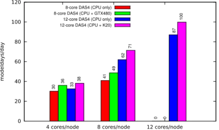
Fig. 10. Performance of POP using eight compute nodes of the DAS-4 cluster, with and without GPUs, using hierarchical
partition-ing with 60×60 block size.
CPU-only version of POP we use the original POP code with the hierarchical partitioning scheme described in Sect. 2.3. Comparisons against other load-balancing schemes can be derived from Fig. 7. All configurations in this section use a block size of 60×60.
Figure 10 shows the performance of POP using 4, 8, and 12 MPI tasks per node, with and without GPU. Note that only a single GPU is available in each node. Therefore, the GPU is shared between the multiple MPI tasks on a single node. For the eight-core DAS-4 nodes, the performance gained by using the GPU is approximately 20 %, both when using four or eight MPI tasks. This directly corresponds with the execu-tion time consumed by POP code that has been ported to the GPU. The figure also shows that the scalability of POP itself is far from perfect. Running on eight MPI task per node, only provides a speed-up of 1.4 compared to four MPI tasks per node, both for the CPU-only and GPU versions.
For the 12-core DAS-4 nodes, the performance gained by using the GPU is approximately 15 % when using 4 MPI tasks per node, and 13 % when using 8 or 12 MPI tasks per node. Although this relative performance gain is lower that for the eight-core nodes, the absolute performance gain is much higher due to the better performance offered by the (newer) six-core CPU and K20 GPUs. In addition, the scal-ability of POP on the 12-core nodes is also much better, achieving a speed-up of 1.9 on 8 cores and 2.6 on 12 cores (both relative to the 4-core experiment).
The results show that it is possible to combine the hier-archical partitioning scheme with GPU execution and still obtain a performance increase. This is a remarkable result, as the hierarchical partitioning scheme prefers small block sizes, such as 60×60, to eliminate as many land-only blocks as possible and distribute load evenly among MPI tasks, while the GPU code would prefer larger-sized blocks to in-crease GPU utilization. However, GPU utilization is already increased by the fact that all MPI tasks running on a single node share a single GPU for all their GPU computations. It is
0 20 40 60 80 100 120
CPU only CPU+GTX480
modeldays/day
Single Cluster DAS4 (16 x 8 cores) Two Clusters DAS4 (2 x 8 x 8 core)
82
94
78
88
Fig. 11.Performance of POP using 16 compute nodes of the DAS-4 cluster, on one or two clusters, using hierarchical partitioning with
60×60 block size.
important to understand that this would not have been possi-ble with larger block sizes because of the limited size of the GPU memory. As such, the two approaches presented in this paper work in concert to improve the performance of POP.
As a final experiment, we study the performance of POP on multiple platforms including GPUs. For this experiment, we use eight-core DAS-4 compute nodes with an Nvidia GTX480 GPU (described in Sects. 3.1 and 5.2).
Figure 11 compares the performance of a 16-node single-cluster run with a 2×8-node two-cluster run. Results are shown for CPU-only and CPU+GPU experiments. The re-sults show a performance increase of 15 % on one cluster and 13 % on two clusters when using the GPUs. The perfor-mance loss when changing from one to two clusters is 5 % for the CPU-only version and 6 % for the CPU+GPU ver-sion. These results clearly indicate that running POP on mul-tiple GPU clusters is feasible and also beneficial in terms of performance. Moreover, it allows users with access to multi-ple smaller GPU clusters to scale up to well beyond the size of a single GPU cluster.
6 Summary, discussion, and conclusions
High-resolution ocean and climate models are becoming a very important tool in climate research. It is crucially im-portant that multi-century simulations with these models can be performed efficiently. In this paper, we presented a new distributed computing approach to increase the performance of the POP model.
of the Zoltan library in order to extend our load-balancing scheme so as to also take performance differences between machines into account. Secondly, it was demonstrated that it is advantageous to port part of POP to GPUs (and get a per-formance increase), even though POP itself does not contain any real hotspots and is therefore not an obvious candidate for using GPUs.
In the experiments shown, only three functions in POP were implemented on a GPU. Another substantial portion of the execution time is spent computing the advection of mo-mentum and the horizontal diffusion of momo-mentum and trac-ers. Obtaining a GPU implementation for these functions is deferred to future work. The advection of tracers also uses the equation of state to compute the potential density refer-enced to the surface layer, which is used to compute a variety of time-averaged fields. Currently, most of the execution time is spent on PCIe transfers. When more computation is moved to the GPU, more data can be reused, and some intermediate data structures that result from computation may even never have to leave the GPU. In that case, some PCIe transfers can be eliminated completely. In future work we hope to produce a complete GPU implementation of the vertical mixing part of POP.
The software presented in this paper has the same portabil-ity properties as the original POP. The GPU code is written in CUDA, which is a widely used language for GPU computing applications. To increase portability across different GPU ar-chitectures, no architecture-specific optimizations have been included. OpenCL is a well-known alternative to CUDA that aims at a wider set of many-core compute devices and differ-ent compilers are available for differdiffer-ent platforms. However, there are no real linguistic differences between CUDA and OpenCL, and porting the code will be a simple engineering effort; furthermore, automated source-to-source translation tools are also available. The use of both extensions (domain decomposition or GPU functions) can be enabled, disabled, and controlled individually through the well-known pop_in namelist file.
Finally, we have shown that the combination of these two approaches also improves performance. Although we demonstrated this only for the DAS-4 cluster, it opens up the possibility to submit a POP job in the near future over multiple supercomputing platforms (with or without GPUs). The new hierarchical load-balancing scheme and the MPI wrapper methodology are crucial elements for maintaining the performance of POP. Future work is to port more of POP to GPUs and to scale up the multi-cluster experiments to pro-duction size hardware.
Acknowledgements. This publication is part of the eSALSA
project (An eScience Approach to determine future Local Sea-level chAnges) of the Netherlands eScience Center (NLeSC), Institute for Marine and Atmospheric research Utrecht (IMAU) at Utrecht University, and VU University Amsterdam. This publication was supported by the Dutch national program COMMIT. Part of the
computations were done on the Huygens IBM Power6 at SURFsara in Amsterdam (www.surfsara.nl). Use of these computing facilities was sponsored by the Netherlands Organisation for Scientific Research (NWO) under the project SH244-13. Support from NWO to cover the costs of this open access publication is also gratefully acknowledged.
Edited by: R. Redler
References
Bleichrodt, F., Bisseling, R., and Dijkstra, H. A.: Accelerating a barotropic ocean model using a GPU, Ocean Model., 41, 16–21, doi:10.1016/j.ocemod.2011.10.001, 2012.
Dennis, J. M.: Inverse space-filling curve partitioning of a global ocean model, IPDPS 2007, IEEE International, 1, 1–10, doi:10.1109/IPDPS.2007.370215, 2007.
Dukowicz, J. K. and Smith, R. D.: Implicit free-surface method for the Bryan-Cox-Semtner ocean model, J. Geophys. Res., 99, 7991–8014, doi:10.1029/93JC03455, 1994.
Kerbyson, D. J. and Jones, P. W.: A performance model of the parallel ocean program, Int. J. High Perform. C., 19, 261–276, doi:10.1177/1094342005056114, 2005.
Khronos Group: OpenCL, available at: http://www.khronos.org/ opencl/ (last access: August 2013), 2013.
Large, W. G., McWilliams, J. C., and Doney, S. C.: Oceanic vertical mixing: a review and a model with a nonlocal boundary layer parameterization, Rev. Geophys., 32, 363–403, doi:10.1029/94RG01872, 1994.
Maassen, J. and Bal, H. E.: Smartsockets: solving the connec-tivity problems in grid computing, in: Proceedings of the 16th IEEE International Symposium on High-Performance Distributed Computing (HPDC), Monterey, CA, USA, 1–10, doi:10.1145/1272366.1272368, 2007.
Maltrud, M., Bryan, F., and Peacock, S.: Boundary impulse re-sponse functions in a century-long eddying global ocean simu-lation, Environ. Fluid Mech., 10, 275–295, doi:10.1007/s10652-009-9154-3, 2010.
Marquet, C. P. and Dekeyser, J. L.: Data-parallel load balancing strategies, Parallel Comput., 24, 1665–1684, doi:10.1016/S0167-8191(98)00049-0, 1998.
McDougall, T. J., Jackett, D. R., Wright, D. G., and
Feis-tel, R.: Accurate and computationally efficient
algo-rithms for potential temperature and density of seawater, J. Atmos. Ocean. Tech., 20, 730–741, doi:10.1175/1520-0426(2003)20<730:AAACEAF>2.0.CO;B2, 2003.
Michalakes, J and Vachharajani, M: GPU acceleration of numerical weather prediction, in: Proceedings of the International Sympo-sium on Parallel and Distributed Processing (IPDPS), IEEE, 1–7, 2008.
Nvidia: CUDA Programming Guide, available at: http://docs. nvidia.com/cuda/ (last access: August 2013), 2013.
Smith, R. D., Maltrud, M. E., Bryan, F. O., and Hecht, M. W.:
Nu-merical simulation of the North Atlantic Ocean at101◦, J. Phys.
Oceanogr., 30, 1532–1561, 2000.
Smith, R., Jones, P., Briegleb, B., Bryan, F., Danabasoglu, G., Dennis, J., Dukowicz, J., Eden, C., Fox-Kemper, B., Gent, P., Hecht, M., Jayne, S., Jochum, M., Large, W., Lindsay, K., Mal-trud, M., Norton, M., Peacock, S., Vertenstein, M., and Yea-ger, S.: The Parallel Ocean Program (POP) Reference Manual: Ocean Component of the Community Climate System Model (CCSM), 2010.
Teresco, J. D., Faik, J., and Flaherty, J. E.: Resource-aware scientific computation on a heterogeneous cluster, Comput. Sci. Eng., 7, 40–50, doi:10.1109/MCSE.2005.38, 2005.
Vallis, G. K.: Atmospheric and Oceanic Fluid Dynamics: Fun-damentals and Large-Scale Circulation, Cambridge University Press, Cambridge, UK, 2006.
Weijer, W., Maltrud, M. E., Hecht, M. W., Dijkstra, H. A., and Kliphuis, M. A.: Response of the Atlantic Ocean circulation to Greenland Ice Sheet melting in a strongly-eddying ocean model, Geophys. Res. Lett., 39, L09606, doi:10.1029/2012GL051611, 2012.
Williams, S., Waterman, A., and Patterson, D.: Roofline: an insight-ful visual performance model for multicore architectures, Com-mun. ACM, 52, 65–76, doi:10.1145/1498765.1498785, 2009. Worley, P. and Levesque, J.: The performance evolution of the
par-allel ocean program on the Cray X1, in: Proceedings of the 46th Cray User Group Conference, 17–21, 2003.