www.nonlin-processes-geophys.net/23/285/2016/ doi:10.5194/npg-23-285-2016
© Author(s) 2016. CC Attribution 3.0 License.
Limiting amplitudes of fully nonlinear interfacial tides and solitons
Borja Aguiar-González1,2and Theo Gerkema3
1Departamento de Física, Facultad de Ciencias del Mar, Universidad de Las Palmas de Gran Canaria, 35017 Las Palmas, Spain
2NIOZ Royal Netherlands Institute for Sea Research, Department of Ocean Systems Sciences, and Utrecht University, P.O. Box 59, 1790 AB Den Burg, Texel, the Netherlands
3NIOZ Royal Netherlands Institute for Sea Research, Department of Estuarine and Delta Systems, and Utrecht University, P.O. Box 140, 4400 AC Yerseke, the Netherlands
Correspondence to:Borja Aguiar-González ([email protected])
Received: 4 January 2016 – Published in Nonlin. Processes Geophys. Discuss.: 19 January 2016 Revised: 22 June 2016 – Accepted: 7 July 2016 – Published: 18 August 2016
Abstract.A new two-fluid layer model consisting of forced rotation-modified Boussinesq equations is derived for study-ing tidally generated fully nonlinear, weakly nonhydrostatic dispersive interfacial waves. This set is a generalization of the Choi–Camassa equations, extended here with forcing terms and Coriolis effects. The forcing is represented by a horizontally oscillating sill, mimicking a barotropic tidal flow over topography. Solitons are generated by a disintegra-tion of the interfacial tide. Because of strong nonlinearity, solitons may attain a limiting table-shaped form, in accor-dance with soliton theory. In addition, we use a quasi-linear version of the model (i.e. including barotropic advection but linear in the baroclinic fields) to investigate the role of the initial stages of the internal tide prior to its nonlinear dis-integration. Numerical solutions reveal that the internal tide then reaches a limiting amplitude under increasing barotropic forcing. In the fully nonlinear regime, numerical experiments suggest that this limiting amplitude in the underlying inter-nal tide extends to the nonlinear case in that interinter-nal solitons formed by a disintegration of the internal tide may not reach their table-shaped form with increased forcing, but appear limited well below that state.
1 Introduction
Tidally generated internal solitons are a widespread phe-nomenon in the oceans and have been observed and stud-ied for decades (see e.g. Apel et al., 2006). They are in-trinsically linked to the internal tide, which itself is
gener-ated by barotropic tidal flow over topography. As the internal tide steepens, it may split up into groups of internal solitons, which therefore appear at the tidal period.
For internal solitons as such, an archetypal model has been the Korteweg–de Vries (KdV) equation, which is based on the assumption of weak nonlinearity and weak nonhydro-staticity. The equation gives prediction for the relation be-tween amplitude, width and phase speed of the solitons, as well as the shape itself. In the KdV equation there is, math-ematically speaking, no limit to the amplitude that solitons may reach (although, of course, at some point the underlying assumption of weak nonlinearity would be violated). This behaviour changes fundamentally if a higher-order (i.e. cu-bic) nonlinear term is included, leading to the so-called ex-tended KdV (eKdV) equation, as discussed in e.g. Helfrich and Melville (2006). This extended version produces qual-itatively different solitons: their amplitude is limited (for a given configuration of layers) and they broaden as they reach their maximum amplitude, the so-called “table-top” solitons. This behaviour is confirmed by fully nonlinear soliton mod-els, as derived by Choi and Camassa (1999) and Miyata (1985, 1988) (denoted as the MCC equations for brevity).
We demonstrate that a saturation in the amplitude of the in-ternal tide occurs, and increasing the barotropic flow further does not produce a larger internal tide. As a consequence, when one includes the genuinely nonlinear effects, i.e. prod-ucts of baroclinic terms, resulting solitons may stay well be-low their formal limiting amplitude, no matter how strong the forcing.
To study these effects we derived a set of fully nonlinear, weakly nonhydrostatic model equations, by extending the MCC equations with a barotropic tidal forcing over topog-raphy and with Coriolis effects, which have previously been shown to play a key role in soliton generation from internal tides (Gerkema and Zimmerman, 1995). To avoid having to deal with nonlinearities in the barotropic tide itself (which cannot be formally neglected in a fully nonlinear model), we mimic the interfacial wave generation, replacing a barotropic tidal flow over topography with a horizontally oscillating to-pography. (There is no exact equivalence between the two, but we demonstrate that, for the parameters used here, the difference remains small.) An alternative approach will also be discussed later.
The presence of a topography greatly complicates the sub-sequent handling of the equations, but we demonstrate that the set of equations can be obtained and can be cast in a form amenable to numerical solving.
An extension of the MCC theory with Coriolis effects (MCC-f) was already derived by Helfrich (2007), who in-vestigated the decay and return of internal solitary waves with rotation. We focus on the novel aspect of studying the wave evolution and limiting amplitudes of fully nonlinear, weakly nonhydrostatic internal tides and solitons when forc-ing and rotational effects are added. We denote our extension of the MCC theory as forced-MCC-f (or forced-MCC in the absence of rotation), for brevity.
The paper is organized as follows. We derive a new two-fluid layer model consisting of a set of forced rotation-modified Boussinesq equations in Sect. 2. We start with the basic equations and assumptions. Then, we scale equa-tions (Sect. 2.1) and vertically integrate them over the layers (Sect. 2.2). Up to this point, the resulting equations are ex-act but do not form a closed set. The set is closed by making an expansion in a small parameter measuring the strength of nonhydrostaticity (Sect. 2.3). The resulting model turns out to be equivalent to the Choi–Camassa equations plus addi-tional terms which represent the forcing and rotation effects. Prior to discussing the numerical experiments, we address in Sect. 3 some aspects related to the oscillating topography, the governing nondimensional parameters and the parameter values used for the runs. In Sect. 4 we investigate the factors limiting the growth of tidally generated solitons by first ex-amining the generation of quasi-linear internal tides within the parameter space of this study. Next, in Sect. 5 we solve the full set of forced-MCC-f and explore the conditions by which tide-generated fully nonlinear solitons may actually
attain a limiting amplitude. The main findings and conclu-sions are presented in Sect. 6.
The numerical methods and schemes are described in Ap-pendix A. The full set of model equations as solved in the code is presented in Appendix B together with its (quasi)-linearized form. In Appendix C we compare, within the pa-rameter space of this study, the case of an oscillating topog-raphy with the case of a tidal flow over a topogtopog-raphy at rest.
2 Derivation of the forced-MCC-f model
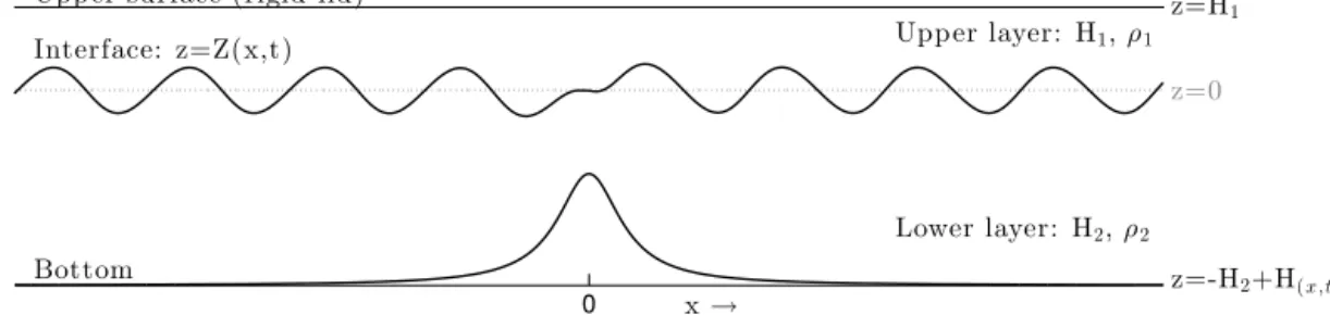
We start from the continuity and Euler equations and con-sider a two-fluid layer system (Fig. 1) with a jump in density across the interface and in which each layer is composed of a homogeneous, inviscid, and incompressible fluid; we apply the Boussinesq approximation. We also assume uniformity in one of the horizontal directions, taking∂/∂y= 0. Hence, the continuity and momentum equations read as
ui,x+wi,z=0, (1)
ρ ui,t+uiui,x+wiui,z−f vi= −pi,x, (2)
vi,t+ui vi,x+wi vi,z+f ui =0, (3)
ρ wi,t+uiwi,x+wi wi,z
= −pi,z−ρi g, (4)
whereρi is density, (ui,vi,wi) are the velocity components
in Cartesian coordinates,pi is pressure,gthe gravitational
acceleration,f the Coriolis parameter (f =2sinφ, at lati-tudeφ) andρthe mean density. The subscripti=1 (i=2) refers to the upper (lower) layer, and a stable stratification,
ρ1< ρ2, is assumed.
Boundaries are defined at the surface, taken to be a rigid lid, which is located atz=H1, and at the bottom, located atz= −H2+H (x, t ). The time dependence of the bottom will later be specified as a horizontal oscillation, mimicking a barotropic tidal flow over topography.
The kinematic boundary conditions at the surface and bot-tom read as
w1 = 0 atz=H1, (5)
w2 = Ht+Hxu2atz= −H2+H (x, t ). (6)
At the interface, z=Z(x, t ), the boundary conditions are given by the continuity of normal velocity and pressure:
wi=Zt+ui Zxandp1=p2atz=Z. (7)
For later convenience, we write pressure as the sum of hydrostatic and dynamic parts, the latter being denoted by primes:
pi=ρ1gH1−ρigz+p′i(t, x, z).
In the horizontal momentum equation, this amounts to re-placingpi,xwithpi,x′ , whereas the vertical momentum
equa-tion (4) gives
ρ wi,t+uiwi,x+wi wi,z
0
Upper surface (rigid-lid) z=H
1
z=0
Interface: z=Z(x,t)
Bottom z=-H2+H
(x,t)
Upper layer: H1,ρ1
Lower layer: H2,ρ2
x→
Figure 1.The two-fluid layer system for which the forced-MCC-f equations are derived. The horizontal dashed grey line indicates the level
z=0, the level at which the interface resides at rest.
The second equation in (7), expressing continuity of pres-sure at the interface, now becomes
(p1′−p′2)|z=Z=(ρ1−ρ2)gZ. 2.1 Scaling
The next step is to bring the equations into an appropriate dimensionless form for which we introduce the following scales. The scale for the undisturbed water depth is taken to be D, and the typical wavelength L. Crucially, we will assume waves to be long, i.e. nonhydrostatic effects to be weak. This will be expressed by the small parameter1,δ=
D L
2
≪ 1.
Since we allow waves to have large amplitudes (i.e. to be strongly nonlinear), we may take horizontal current veloci-ties to scale withc0=(g′D)1/2, whereg′is reduced gravity,
g′=g (ρ2−ρ1)/ρ. (Notice that the exact linear long-wave phase speed for interfacial waves,cp, is similar toc0, but has
H1H2/Dinstead ofDin the square root.) Thus,uandvwill be scaled withc0. As the interfacial displacement is allowed to be large, an appropriate scale ofZisD.
The typical scale of w now follows from the continuity equation as Dc0/L. Finally, the scale of pressure follows from assuming a primary balance between the acceleration termsρ ut andpxin the horizontal momentum equation.
In summary, then, we can introduce the following dimen-sionless variables, indicated by asterisks,
x=L x∗, z=D z∗, t=(L/c0) t∗, p′i=(ρ c20) p′∗i,
ui=c0u∗i, vi=c0v∗i, wi=(D/L) c0wi∗. (8)
With these scales, the dimensionless continuity and Euler equations yield (for convenience, we drop the asterisks right away)
ui,x+wi,z=0, (9)
ui,t+ui ui,x+wi ui,z−µ vi= −p′i,x, (10)
vi,t+ui vi,x+wi vi,z+µ ui=0, (11)
1In Choi and Camassa (1999) a small parameterǫwas used
in-stead, which relates to ours asδ=ǫ2.
δ wi,t+uiwi,x+wi wi,z
= −pi,z′ . (12)
Hereµis the scaled Coriolis parameter,µ=f L/c0. Further-more, we introduce the dimensionless quantitiesζ,hi, andh
via(Z, H1, H2, H )=D(ζ, h1, h2, h), so that the scaled form of the boundary conditions is
w1=0 atz=h1, (13)
wi=ζt+ui ζxatz=ζ (x, t ), (14)
p′2−p1′ =ζ atz=ζ (x, t ), (15)
w2=ht+u2hxatz= −h2+h(x, t ). (16)
The goal is now to derive a reduced set of equations from Eqs. (9) to (12), in which the boundary conditions (13)–(16) are incorporated by vertical integration, exploiting the small-ness of the parameterδ. The procedure is identical to that of Choi and Camassa (1999), but with the additional complica-tions of the Coriolis force, topography, and tidal forcing. 2.2 Vertically integrated equations
We vertically integrate the equations over the upper and lower layers and expand them to the ordersδ0andδ1to ob-tain a closed set for the weakly nonhydrostatic equations, fol-lowing Choi and Camassa (1999). The layer meanf1 of a functionf1(x, z, t )for the upper layer is defined as
f1(x, t )= 1
η1
h1
Z
ζ
dzf1(x, z, t ), η1=h1−ζ , (17)
and for the lower layer as
f2(x, t )= 1
η2
ζ
Z
−h2+h
dzf2(x, z, t ), η2=h2−h+ζ, (18)
whereηi represents the thickness of the layer (depending
on the interfacial displacement ζ). Notice that the bound-aries of the integral depend on time and space (x) via the interfacial movementζ (t, x), but also, for the lower layer, via the horizontally oscillating topography2,h(t, x). Before 2For this reason we need to apply the Leibniz integral rule below
proceeding, nonlinear terms in the horizontal momentum equations (10) and (11) are rewritten as(u2i)x+(wiui)zand
(uivi)x+(wivi)z, respectively, to facilitate the procedure.
After integration of Eqs. (9)–(11) fori=1 and applying the boundary conditions (13)–(15), we obtain the layer-mean equations for the upper layer:
η1,t+(η1u1)x=0, (19)
(η1u1)t+(η1u1u1)x−µη1v1= −η1p′1,x, (20)
(η1v1)t+(η1u1v1)x+µη1u1=0. (21) For the lower layer one proceeds similarly, except that now both boundaries are variable. Applying the boundary condi-tions (14)–(16), vertical integration of Eqs. (9)–(11) fori=2 yields
η2,t+(η2u2)x=0, (22)
(η2u2)t+(η2u2u2)x−µη2v2= −η2p′2,x, (23)
(η2v2)t+(η2u2v2)x+µη2u2=0. (24) 2.3 Expansion inδ
The six integrated Eqs. (19)–(24) derived so far are exact but do not form a closed set. The variablesη1,η2andζ count as one unknown, but we also haveui,vi,p′i,x,uiui anduivi,
giving 11 unknowns for 6 equations. To obtain a closed set, the last two expressions will be cast in terms ofui andvi by
using the vertical momentum equation, expanded in terms of the small parameterδ. Furthermore, continuity of pressure at the interface is used to connect the pressure in the lower and upper layers (i.e.p′1,x andp2′,x). All in all, the six equations are thus modified to contain only six unknowns. With this aim, we make a formal expansion of the unknowns for the lowest (δ0) and next (δ) orders, as, for example,
fi=fi(0)+δfi(1)+. . .
At the lowest order (δ0),p′(0), the dynamics is hydrostatic. At the next order (δ),p′(1)brings weakly nonhydrostatic ef-fects into the system.
2.3.1 Lowest order
At lowest order, the vertical momentum equation (12) re-duces to ∂p′i(0)/∂z=0 as terms of orderδ are neglected; therefore, (perturbation) pressure is vertically constant in each layer. For convenience, we introduceP =p2′(0), being a function oftandx. It then follows from continuity of pres-sure at the interface thatp1′(0)=P−ζ. Thus, to this order of approximation,
p′1,x =Px−ζx+O(δ), (25)
and, for the lower layer,
p′2,x =Px+O(δ). (26)
Given thezindependence of pressure and returning to the original horizontal momentum equations, it is now natural to assume that the horizontal velocities, too, are independent of
zwithin each layer:
uiui=u2i +O(δ), uivi=uivi+O(δ).
At lowest order, then, the set of integrated equations is closed; together with the (exact) integrated continuity equa-tions (19) and (22), we have the momentum equaequa-tions in terms of the six variablesui,vi,ζ andP:
(η1u1)t+(η1u21)x−µη1v1= −η1(Px−ζx)+O(δ), (27)
(η2u2)t+(η2u22)x−µη2v2= −η2Px+O(δ), (28)
(η1v1)t+(η1u1v1)x+µη1u1=O(δ), (29)
(η2v2)t+(η2u2v2)x+µη2u2=O(δ). (30) Recall thatη1,2can be expressed in terms ofζ and thus involve just one unknown.
2.3.2 Next order
At order δ, the procedure is to close the set of six verti-cally integrated equations by deriving expressions for the horizontal pressure gradientsp′i,x as well as for the contri-butions ofuiui anduivi in the nonlinear terms. The latter
problem is particularly simple. At orderδ, the products con-tain one lowest-order field, which is independent ofz(e.g.
ui(0)=ui(0)); hence,
uiui=
1
ηi
Z
dz u2i = 1
ηi
Z dz
ui(0)
2
+2δui(0)ui(1)+. . .
= ui(0)
2
+2δui(0)ui(1)+. . .
= u2i +O(δ2),
so that
uiui=u2i +O(δ
2), u
ivi=uivi+O(δ2).
This allows us to write the horizontal momentum equa-tions as
(η1u1)t+(η1u21)x−µη1v1= −η1(p1′ (0)+δp′
1 (1))
x+O(δ2), (31) (η2u2)t+(η2u22)x−µη2v2= −η2(p2′
(0)+δp′ 2
(1))
x+O(δ2), (32) (η1v1)t+(η1u1v1)x+µη1u1=O(δ2), (33) (η2v2)t+(η2u2v2)x+µη2u2=O(δ2). (34) The remaining problem is to find an expression forp′i(1). At orderδ, Eq. (12) reads, in terms of the lowest-order verti-cal velocities,
wi(0)t+ui(0)wi(0)x+wi(0)wi(0)z= −pi′ (1)
z. (35)
By vertically integrating the continuity equation (9), we obtain an expression forwi(0):
whereciare “constants” of integration which are determined
by using the boundary conditions at the surface (13) and bot-tom (16). Thus,wi(0)for the upper and lower layers become,
respectively,
w1(0) = (h1−z) u1,x(0), (36)
w2(0) = (h−h2−z) u2,x(0)+D2h, (37) where the operatorDi is defined as∂/∂t+ui(0)∂/∂x.
Sub-stituting w1(0) from Eq. (36) andw2(0) from Eq. (37) into Eq. (35), and vertically integrating the result, we get an ex-pression forp′
1
(1)
andp′
2
(1)
. Taking their derivative with re-spect toxand their mean over each layer, we finally obtain an expression for p′i(1)x at orderδ. Including the lowest-order terms (25) and (26), this allows us to write the horizontal pressure gradient for the upper layer,
p′1,x = p′1,x(0)+δp1′,x(1)+O(δ2)
= Px−ζx−δ
1 3η1
(η31G1)x
+O(δ2), (38)
and, for the lower layer,
p′2,x = p′2,x(0)+δp2′,x(1)+O(δ2)
= Px−δ
1 3η2
(η23G2)x+
1 2η2G2hx
− η2
2(D 2
2h)x−ζxD22h i
+O(δ2), (39)
where we introduced for simplicity the termGi (as in Choi
and Camassa, 1999),
Gi=ui,xt(0)+ui(0)ui,xx(0)−(ui,x(0))2. (40)
With this, the horizontal momentum equations (31) and (32) become
(η1u1)t+(η1u21)x−µη1v1
= −η1
n
Px−ζx−δ
1 3η1
(η31G1)x
o
+O(δ2) (41)
(η2u2)t+(η2u22)x−µη2v2
= −η2
Px−δ
1 3η2
(η32G2)x+
1 2η2G2hx
−η2
2(D 2
2h)x−ζxD22h io
+O(δ2). (42)
We have thus obtained a closed set of six dimensionless equations, namely the exact continuity equations (19) and (22), the horizontal momentum equations (41) and (42), as well as (33) and (34); the last four equations involve the weakly nonhydrostatic assumption. The six unknowns are
u1,u2,v1,v2,P, and (viaη1,2)ζ. Without interfacial forcing
and Earth’s rotation, our set of equations correctly reduces to that of Choi and Camassa (1999). We further specify the
model by prescribing the oscillating topography, i.e. the forc-ing to the system, with
h=h(X)whereX(x, t )=x−U0cost, (43) andU0is an arbitrary positive constant.
We combine the continuity equations (19) and (22) into
(η1+η2)t+(η1u1+η2u2)x=0. (44)
Given thatη1+η2=h1+h2−h, with the two-fluid system depthh1+h2=1, this leads to
−ht+(η1u1+η2u2)x=0. (45)
If we now substitute the time derivative of the oscillating topography (43), we have
(η1u1+η2u2)x=U hx, (46)
with
U =U0sin t, (47)
which is the velocity of the oscillating topography with am-plitudeU0, mimicking a barotropic tidal flow. However, the two are not exactly equivalent, since the transformation from one frame of reference to the other involves an acceleration, and is therefore not Galilean. We discuss this aspect further in Appendix C.
Equation (46) can be then integrated inx:
η1u1+η2u2=U h+C(t ). (48)
Far from the sill (i.e.h→0 forx→ ±∞), we impose the flow to be purely baroclinic, so that the left-hand side must be zero, and hence it follows thatC(t )=0. Notice that the right-hand side is prescribed via the forcing and thus is a known quantity. It allows us to expressu2in terms ofu1.
We can thus combine the horizontal momentum equa-tions (41) and (42), eliminatingP,
u1,t + u1u1,x+µv1=ζx+
1
(1−h)
(U h)t+(η1u21+η2u22)x
− µ(η1v1+η2v2)−η1ζx
+δ
1− η1
(1−h)
"
η1G1η1,x+
η21
3G1,x #
+ δη2
(1−h)
"
−η2G2ζx−
η22
3 G2,x
+ η2G2
2 hx+
η2 2 (D
2
2h)x+ζxD22h
+O(δ2) (49)
u2=
U h−η1u1
η2
v1,t+u1v1,x+µu1=O(δ2), (51)
v2,t+u2v2,x+µu2=O(δ2), (52)
ζt−(h1−ζ )u1,x+u1ζx=0, (53)
where thevi-horizontal momentum equations (51) and (52)
have been further simplified from Eqs. (33) and (34) by us-ing the continuity equations (19) and (22). Equation (19) has now been expressed in terms ofζ for convenience. The other continuity equation (22) is no longer included since it is al-ready implicitly present via Eq. (50).
All in all, we now have five equations for five unknowns (u1,u2,v1,v2andζ). The numerical methods and schemes used to solve the model are described in Appendix A. The actual form of the model equations as used in the numerical code is presented in Appendix B. In Appendix C we com-pare, within the parameter space of this study, the case of an oscillating topography with the case of a tidal flow over a topography at rest.
Before concluding this section, it is worthwhile noting an alternative approach. Given the assumption of a rigid lid, one could have also takenU=0 in Eq. (48), the topographic mo-tion set to zero, and then prescribed an external barotropic flux viaC(t ). Imposing a barotropic flux in this manner does not allow for spatial variations of that flux, as would occur with a free surface, for which an additional dynamical equa-tion would be required to solve the barotropic mode. Speci-fication ofC(t )is common in fully nonlinear models of this type as, for example, in Lamb (1994) and Vlasenko et al. (2005). However, the choice of an oscillating topography has also proven to be of use in the study of strongly nonlinear interfacial waves. For instance, Grue (2015) recently con-firmed findings on the onset of wave train formation observed in experimental measurements by Maxworthy (1979) with a three-dimensional two-layer, fully dispersive and strongly nonlinear interfacial wave model with a time-varying bottom topography.
3 Numerical experiments: preliminary remarks Whilst not designed to represent a specific region of the world oceans, we aim to investigate in a general manner the conditions by which tidally generated solitons may evolve and, eventually, develop limiting amplitudes in ocean-like scenarios. It is then desirable that leading solitons can propa-gate towards a mature stage before overtaking preceding in-ternal tides; otherwise, although these are form-preserving features, the tracking of their wave properties becomes cum-bersome. For this reason, the parameters that we describe in the following were selected to highlight the qualitative fea-tures of these nonlinear processes for a broad range of (mim-icked) tidal forcing strengths.
Although the model is solved and discussed in nonsional form, we also present the parameter values in dimen-sional form to put them in an oceanographic context.
3.1 The oscillating topography and the hydraulic state: the Froude number
We define the (dimensional) topography analytically follow-ing
H (X)= HT
1+(x/HL)2
, (54)
withx being the grid positions in space, and HT and HL
being the dimensional parameters which set the height and width of a symmetric sill, respectively. In this manner we ensure perfectly smooth second and third derivatives of the dimensionless topographyh(X)in the model equations.
At this point it is worthwhile recalling that the oscillation of the topography is introduced in dimensionless form ash=
h(X) withX(x, t )=x−U0cost, where U0 prescribes the strength (velocity amplitude) of the oscillating topography viaU=U0 sin(t ), the mimicked barotropic tidal flow (see Eqs. 43–47). By increasingU0 we enhance the forcing via
U, which in dimensional form we introduce, respectively, as U0=c0U0andU=c0U.
The topographic obstacle (ridge, sill, etc.) is always cen-tered on thex axis and the length of the x domain is cho-sen to be large enough to prevent waves from reaching the boundaries. In all experiments, the topography starts mov-ing to the left at t=0; we start with a system at rest, i.e.
U=u1=u2=0 att=0. The waves are generated near the origin; on the negative (positive)x axis, waves travel to the left (right). Because the forcing starts asymmetrically, it is expected that wave packets in the front appear rather differ-ently when comparing both sides (negative vs. positivex do-main). These fronts are the transients, which are influenced by the way the experiment is started. A steady solution at both sides of thex axis is reached after several tidal peri-ods have passed. In this regard, and to avoid transient effects generated at the start of each run, wave properties have been tracked systematically for the third leftward-propagating in-terfacial wave counting from the front and after nine tidal periods of forcing.
To characterize the hydraulic state, we use the Froude number calculated as
F r=U0
cp
, (55)
where the amplitude of the mimicked tidal flow,U0, is com-pared to the linear long-wave phase speed for interfacial waves,cp. The strength ofU0leads to three different regimes of interfacial wave generation (see e.g. Vlasenko et al., 2005; Da Silva et al., 2015). Accordingly, the hydraulic regime is denoted, hereafter, as subcritical whenFr≪1, critical when
Fr≈1, and supercritical when Fr>1. To account for the varying strength of the tidal forcing within a tidal cycle, we introduce the instantaneous Froude number, defined as
Importantly, we also use the Froude number in Ap-pendix C to discuss the applicability of our “non-inertial” frame of reference, the oscillating topography, to the ocean case, where the topography is at rest. To this aim we compare the generation of interfacial waves from the (quasi-)linear forced-MCC equations with that from the (quasi-)linear ver-sion of the weakly nonlinear model derived in Gerkema (1996), which works with actual tidal motion. Recall that in the quasi-linear case, barotropic advection is retained but baroclinic interactions are neglected. The equations are then still linear with regard to the baroclinic fields, but the co-efficients become time-dependent due to barotropic factors (which are prescribed), so that higher harmonics will be gen-erated when the forcing is increased. For clarification, the (quasi-)linearization of the forced-MCC-f equations is pre-sented in Appendix B.
Results from this model comparison confirm a near equiv-alence between both models within the parameter framework of study, which we restrict to 0< F r <1.6. This encourages us to discuss our numerical results, henceforth referring to the strength of the topographic oscillation,U0, as the strength of the tidal flow.
3.2 Parameter values
We adopt a two-layer system where the total water depth,
D, is set to 100 m, with the upper layer always being thin-ner than the lower layer (H1< H2). The horizontal oscilla-tion of the moving topography is always of semidiurnal fre-quency. Although the height of the topography varies be-tween runs, its horizontal scale is kept constant and about 20 km (HL=10 km in Eq. 54). Regarding reduced
grav-ity, g′ typically ranges from 0.007 m s−2 in the Celtic Sea (Gerkema, 1996) to 0.027 m s−2 over the Oregon continen-tal shelf (Stanton and Ostrovsky, 1998); we use this range accordingly.
In Table 1 the varying parameters are listed. They vary be-tween runs as indicated in bold fonts, one at a time. The the-oretical amplitude of the “table-top” soliton predicted from Eq. (3.68) in Choi and Camassa (1999), and beyond which no solitary wave solution exists, is also indicated.
In Sect. 4, runs A1, A2 and A3 illustrate the effect of vary-ing stratification via the reduced gravity, g′. Runs A1, B1 and B2 illustrate the effect of varying the topography ratio,
ϕT =HT/D, the height of the topography relative to the total
water depth. Finally, runs A1, C1 and C2 illustrate the effect of varying the two-fluid layer thickness ratio, γ=H1/H2. Based on the results from the above analyses, we will argue later why in Sect. 5 we focus on a highly stratified regime (g′=0.03 m s−2) for the study of fully nonlinear waves.
For convenience, wave properties are scaled as follows. The interfacial displacement,Z, the internal tide amplitude,
A, and the soliton amplitude, As, are scaled to the thick-ness of the upper layer, H1. The soliton phase speed, cs, is scaled to the phase speed of linear long-wave interfacial
waves,cp. Horizontal distances along thex-direction and the soliton width,Ls, are scaled to the wavelength of linear long-wave interfacial long-waves,Lp. Finally, we use the scaled Cori-olis parameter,µp, which relates toµin Sect. 2.1, following
µp=µ/(2π ).
4 Numerical experiments: quasi-linear internal tides Tide-generated solitons emerge from nonlinear disintegra-tion of the underlying internal tides and may be, therefore, naturally subjected to the properties of the latter. For this rea-son, we find it insightful to investigate first the properties of the underlying internal tides, prior to their nonlinear disinte-gration, within the parameter space of this study.
As described in Sect. 3, the quasi-linear case includes ad-vective terms from the interactions between the barotropic and baroclinic flows, while interactions between baroclinic fields, the genuinely nonlinear terms, are still absent. There-fore, higher harmonics are naturally generated when the forc-ing is increased. The linear case, where all advective terms are absent, is included here to assess potential departures from the quasi-linear case.
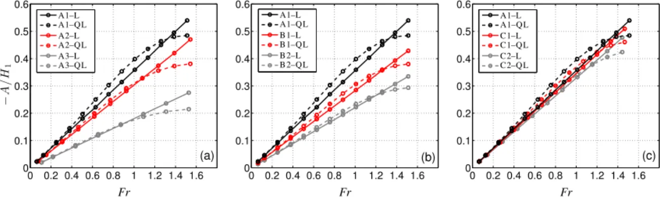
Accordingly, Fig. 2 presents the internal tide response to the strength of the tidal forcing for runs A1 to C2 (see Table 1). The minimum forcing strength for all cases is U0=5 cm s−1. In subsequent data points, the increase inU0 is 10 cm s−1fromU0=10 cm s−1and onwards, reaching up toFr∼1.5.
In the purely linear experiments, the amplitude of the in-ternal tide increases linearly with the barotropic tidal flow strength. However, the quasi-linear internal tide exhibits a limiting amplitude in all runs, when the tidal forcing in-creases well above F r=1, a feature that seems to have passed unnoticed in earlier studies. For weak forcing (F r≪
1), the amplitude of the quasi-linear internal tides approaches the linear case; the advective terms then become very small. This pattern indicates that the decisive factor in the amplitude saturation of quasi-linear internal tides lies in the barotropic advection, which is absent in the linear case.
0 0.2 0.4 0.6 0.8 1 1.2 1.4 1.6 0
0.1 0.2 0.3 0.4 0.5 0.6
(a)
Fr
−
A
/
H
1
A1–L A1–Q L A2–L A2–Q L A3–L A3–Q L
0 0.2 0.4 0.6 0.8 1 1.2 1.4 1.6 0
0.1 0.2 0.3 0.4 0.5 0.6
(b)
Fr A1–L A1–Q L B 1–L B 1–Q L B 2–L B 2–Q L
0 0.2 0.4 0.6 0.8 1 1.2 1.4 1.6 0
0.1 0.2 0.3 0.4 0.5 0.6
(c)
Fr A1–L A1–Q L C1–L C1–Q L C2–L C2–Q L
Figure 2.Amplitude of the linear,L, and quasi-linear,QL, internal tide scaled to the thickness of the upper layer vs. the Froude number.
Varying parameters between panels are(a)the strength of stratification,g′(runs A1, A2 and A3);(b)the topography ratio,ϕT (runs A1, B1
and B2); and(c)the two-fluid layer thickness ratio,γ(runs A1, C1 and C2). The run time is nine tidal periods. See Table 1 for further details.
Table 1.Summary of runs. Varying parameters are the reduced gravity,g′(m s−2), thetopography ratio,ϕT, and thetwo-fluid layer thickness
ratio,γ. The theoretical maximum amplitude,Am, as predicted from Eq. (3.68) in Choi and Camassa (1999), is also indicated.
Run g′ ϕT =HT/D γ=H1/H2 −Am/H1 H1,H2 ρ1,ρ2
(in m s−2) (in m) (kg m−3)
A1 0.03 0.4 0.43 0.67 30, 70 1022, 1025.15
A2 0.02 0.4 0.43 0.67 30, 70 1023.05, 1025.15
A3 0.01 0.4 0.43 0.67 30, 70 1024.1, 1025.15
B1 0.03 0.35 0.43 0.67 30, 70 1022, 1025.15
B2 0.03 0.3 0.43 0.67 30, 70 1022, 1025.15
C1 0.03 0.4 0.33 1 25, 75 1022, 1025.15
C2 0.03 0.4 0.25 1.5 20, 80 1022, 1025.15
Although not shown, it is worth mentioning that the wave-length of the quasi-linear tides does not deviate from the lin-ear case in any of the settings of study and is independent of the strength of the tidal forcing (and hence of the Froude number) and of the height of the topography. However, as predicted from linear theory for interfacial waves, an increase ing′orH1(withH1< H2andDbeing constant) generates longer internal tides.
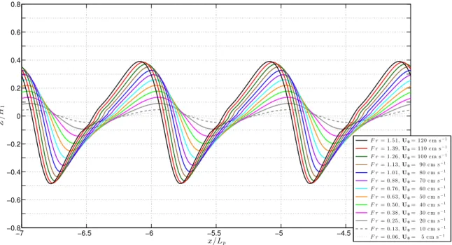
The amplitude saturation described above is further illus-trated in Fig. 3 for run A1, where snapshots of leftward-propagating quasi-linear internal tides are shown for various forcing strengths (see legend). This spatial view shows how the increase in the forcing transforms the wave from a sinu-soidal to an asymmetric shape, indicative of the presence of higher harmonics, while the amplitude becomes saturated.
These findings raise the question as to whether solitons emerging from a disintegration of the initially quasi-linear in-ternal tides may be subjected to saturation before they reach a limiting “table-top” shape. We examine this question in the next section by focussing on runs A1, B1 and C1, varying the height of the topography and the thickness of the upper layer while preserving a high stratification. The latter allows us to investigate the broadest range of interfacial wave amplitudes, as suggested by Fig. 2a.
5 Numerical experiments: fully nonlinear internal tides and solitons
In this section we investigate the conditions by which tidally generated fully nonlinear solitons may attain a limiting am-plitude. Special attention is devoted to factors conditioning the growth of fully nonlinear waves as “table-top” solitons. The main question to address is whether the amplitudes of tidally generated solitons may be subjected to limiting am-plitudes of the underlying quasi-linear internal tides, as we hypothesized in the previous section, thus qualifying predic-tions from classical eKdV and MCC theories.
5.1 Tide-generated “table-top” solitons: run A1
−7 −6.5 −6 −5.5 −5 −4.5 −4 −0.8
−0.6 −0.4 −0.2 0 0.2 0.4 0.6 0.8
Z
/
H1
x/Lp
F r= 1.51,U0= 120 c m s−1
F r= 1.39,U0= 110 c m s−1
F r= 1.26,U0= 100 c m s−1
F r= 1.13,U0= 90 c m s−1
F r= 1.01,U0= 80 c m s−1
F r= 0.88,U0= 70 c m s−1
F r= 0.76,U0= 60 c m s−1
F r= 0.63,U0= 50 c m s−1
F r= 0.50,U0= 40 c m s−1
F r= 0.38,U0= 30 c m s−1
F r= 0.25,U0= 20 c m s−1
F r= 0.13,U0= 10 c m s−1
F r= 0.06,U0= 5 c m s−1
Figure 3. Snapshots of the interfacial displacement of leftward-propagating quasi-linear internal tides for run A1 (H1=30 m;
Lp=35.49 km). The amplitude saturation is evident as the tidal forcing is increased and the flow becomes supercritical (see legend). The run
time is nine tidal periods.
At a first stage, Fig. 4b, the internal tide splits up into two different groups of rank-ordered solitons: a train of de-pressions on the leading edge, and a train of elevations, af-ter the former packet, with initially smaller amplitudes. At a later stage, Fig. 4c, the largest elevations have reached the smaller depressions in the train, and three leading solitons at the front present almost equal amplitudes. Previous solitary wave packets, already propagating away from the generation area, are shown in Fig. 4d and e and correspond to preceding disintegrated internal tides. The “table-top” soliton observed at the leading edge of every preceding internal tide emerged in all cases from the first of the three solitons described pre-viously in Fig. 4c.
As the leading soliton evolves and reaches its maximum amplitude, it also broadens, as predicted by soliton wave the-ory (Helfrich and Melville, 2006), in comparison with subse-quent solitons of smaller amplitude (Fig. 4d, e). The observed increase in the distance between the “table-top” soliton and subsequent (smaller) solitons also indicates that, as expected from theory, the leading soliton moves (phase speed) faster than solitons in the tail.
Because tidally generated solitons are part of the evolving internal tides, z=0 cannot be used as a reference level to compute the amplitude down to the trough of the soliton (see Figs. 1 and 4). Similarly, the soliton width cannot be mea-sured takingz=0 as a reference level. A criterion is required to adopt a suitable reference level for calculating the soliton amplitude,As, and width,Ls. Here we introduce the refer-ence levelZa, which for every leftward-propagating soliton
indicates where the first spatial derivative of the interfacial
displacement,Z, becomes zero. Accordingly, the soliton am-plitude,As, is defined as the vertical distance betweenZaand
the trough of the leading soliton, located atZb (see e.g. in
Fig. 4c–e). The soliton width,Ls, is defined as the horizontal distance betweenZcandZd, located halfway of the vertical
distance spanningAs(see also e.g. in Fig. 4c–e). Finally, the soliton phase speed,cs, is computed by subtracting the ve-locity of the (mimicked) tidal flow,U, from the velocity of the soliton embedded within the internal tide.
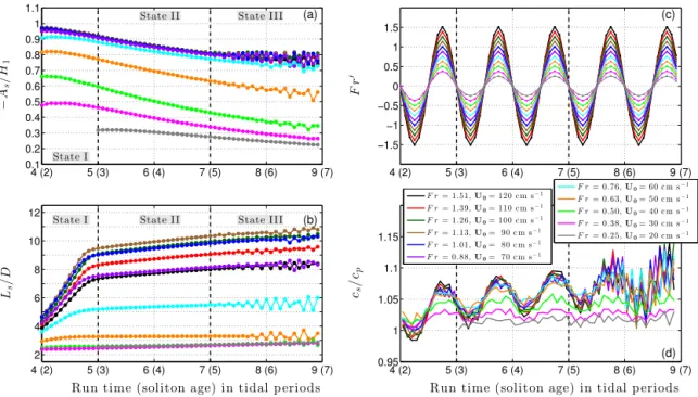
Using the above criteria, Fig. 5 presents the wave evolution of leading solitons under different forcing strengths (see leg-end) towards a fully developed stage. Contrary to what one might expect, the amplitudes of the leading solitons decrease during their evolution (Fig. 5a). This can be ascribed to their tide-generated nature. At an early stage, the disintegration of the internal tide leads at its front to a large depression, and this subsequently evolves into a mature leading soliton prop-agating through the tail of the preceding internal tide (see Fig. 4c–e).
The soliton reaches its maximum amplitude slightly before the flow becomes critical (Fr=0.88) and attains the “table-top” form in the supercritical regime when forced with a stronger tidal flow (Fr=1.13). Unexpectedly, when the tidal forcing is increased even further, the soliton width starts to decrease while keeping its maximum amplitude (cf. Fig. 5a and b). This feature is unlike classical eKdV and MCC the-ories, suggesting that limiting factors related to the forcing may be acting.
−7 −6 −5 −4 −3 −2 −1 0 −0.8
−0.4 0 0.4
Z
/
H1
(a)
−1 −0.75 −0.5 −0.25 0
−0.8 −0.4 0 0.4
(b)
Z
/
H1
−2 −1.75 −1.5 −1.25 −1
−0.8 −0.4 0 0.4
Z
/
H1
(c)
−4 −3.75 −3.5 −3.25 −3
−0.8 −0.4 0 0.4
Z
/
H1
(d)
−6.2 −5.95 −5.7 −5.45 −5.2
−0.8 −0.4 0 0.4
Za
Zb
Zc
Zd
x/Lp
Z
/
H1
(e)
Figure 4.Snapshots of the interfacial displacement of nonlinear internal tides and solitons in run A1 for a supercritical regime (Fr=1.13,
U0= 90 cm s−1).(a)Overview of leftward-propagating internal tides and solitons.(b–e)Set of spatial zooms from(a)showing different
stages of the nonlinear disintegration of the internal tides. PointsZa(black dot),Zb(grey dot),Zc(black square) andZd(grey square) are
shown to illustrate how the soliton amplitude,As, and width,Ls, are computed (see the text in Sect. 5.1 for details). The run time is nine
tidal periods. For scaling purposes we recall that, for run A1,H1=30 m andLp=35.49 km.
4 (2) 5 (3) 6 (4) 7 (5) 8 (6) 9 (7) 0.1
0.2 0.3 0.4 0.5 0.6 0.7 0.8 0.9 1 1.1
State I
State I I State I I I (a)
−
As
/H
1
4 (2) 5 (3) 6 (4) 7 (5) 8 (6) 9 (7) 2
4 6 8 10 12
Ls
/D
Run time (soliton age) in tidal p eriods
State I State I I State I I I (b)
4 (2) 5 (3) 6 (4) 7 (5) 8 (6) 9 (7) 0.95
1 1.05 1.1 1.15
cs
/c
p
Run time (soliton age) in tidal p eriods
(d)
F r= 0.76,U0= 60 c m s−1 F r= 0.63,U0= 50 c m s−1 F r= 0.50,U0= 40 c m s−1 F r= 0.38,U0= 30 c m s−1 F r= 0.25,U0= 20 c m s−1
4 (2) 5 (3) 6 (4) 7 (5) 8 (6) 9 (7) −1.5
−1 −0.5 0 0.5 1 1.5
Fr
′
(c)
F r= 1.51,U0= 120 c m s−1 F r= 1.39,U0= 110 c m s−1 F r= 1.26,U0= 100 c m s−1 F r= 1.13,U0= 90 c m s−1 F r= 1.01,U0= 80 c m s−1 F r= 0.88,U0= 70 c m s−1
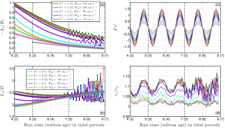
Figure 5.Wave evolution of leftward-propagating leading solitons in run A1 under different forcing strengths (see legend). In all panels
the horizontal axis indicates the run time and soliton age (in brackets) in tidal periods. The (dimensionless) wave properties are(a)soliton amplitude,As/H1;(b)soliton width,Ls/D;(c)instantaneous Froude number,Fr′=U/cp; and(d)soliton phase speed,cs/cp. Note that we
takecpto be negative (leftward propagation) for consistency with the physical meaning of the sign inFr′. For scaling purposes, we recall
b). First, the smaller and narrower solitons, generated in a subcritical regime and which attain a nearly constant shape quickly after their generation (Fr60.5). Second, the larger and broader solitons, generated in nearly critical and su-percritical regimes and which evolve over longer timescales (Fr>0.88). We distinguish here three different states for strongly nonlinear solitons, which are indicated with vertical dashed lines and labels in Fig. 5a and b. During State I emerg-ing solitons evolve as transient waves which broaden linearly until they reach a fully developed form. Then, in State II, they preserve their shape in time and, occasionally, may overtake the preceding internal tide, which is State III, causing the os-cillations observed in the width, amplitude and phase speed in Fig. 5a, b, and d.
In agreement with the above description, the phase speed graphs also reveal a clear distinction between the subcritical and critical/supercritical regimes (Fig. 5d). On the one hand, smaller solitons show a nearly constant phase speed. They were generated with a small or moderate tidal forcing (sub-critical flow). On the other hand, larger solitons present an oscillating phase speed which increases over time. They were generated with a relatively strong tidal forcing (critical and supercritical flow). The oscillation is the response to a gov-erning flow where the accelerating and decelerating phases of the soliton are imposed by the direction of the tidal flow. This is seen by comparing the instantaneous Froude number,Fr′, in Fig. 5c with the soliton phase speed in Fig. 5d. Crucial mo-ments occur whenFr′= −1 and Fr′<−1. During the for-mer, solitons cannot propagate against the tidal flow, and re-main stationary. During the latter, leftward-propagating soli-tons experience a rightward advection driven by the larger tidal flow.
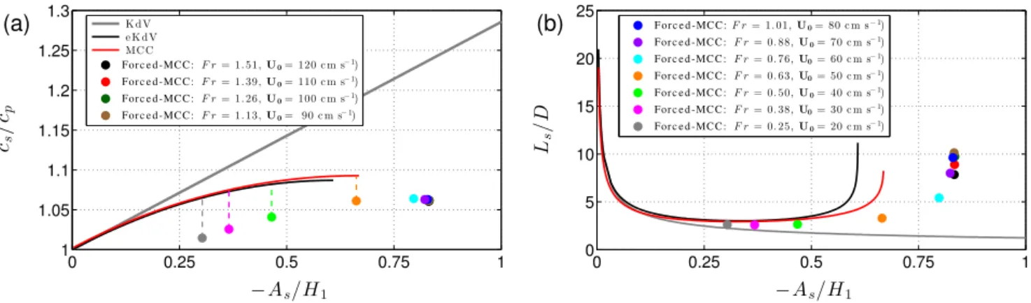
Finally, we compare in Fig. 6 the wave properties of ma-ture forced-MCC solitons3 with KdV-type and MCC soli-ton solutions (Kakutani and Yamasaki, 1978; Ostrovsky and Stepanyants, 1989; Miyata, 1985, 1988; Choi and Camassa, 1999; Helfrich and Melville, 2006; Gerkema and Zimmer-man, 2008). To this aim, the soliton width for KdV-type and MCC theories is computed following the same procedure as for the forced-MCC solitons; that is, we use points Zc and
Zd(see Fig. 4c–e).
As expected, small tide-generated solitons approach the linear long-wave phase speed for interfacial waves (cs/cp≈ 1), while larger tide-generated solitons have a higher phase speed following a curve as in eKdV and MCC theory. How-ever, because tide-generated solitons ride on internal tides, their wave properties are not simply the response to a two-fluid layer system as such, as happens for eKdV and MCC solitons, but they are also subjected to the forcing of the sys-tem and to a variable background flow (the internal tide). We suggest that the above scenario may account for the slower phase speeds of the forced-MCC solitons when compared to 3These wave properties correspond to solitons of State II
(ma-ture solitons) after time averaging over a tidal cycle.
their eKdV and MCC counterparts. Interestingly, this differ-ence slightly decreases as the solitons grow (cf. the length of the coloured dashed lines in Fig. 6a).
As regards the relationship between the soliton width and amplitude, tide-generated solitons follow a similar behaviour to that predicted by eKdV and MCC theory, broadening as they approach their maximum amplitude. By this broad-ening, strongly nonlinear solitons develop the “table-top” shape, although forced-MCC equations generate some larger and narrower solitons than their eKdV and MCC counter-parts (Fig. 6b).
5.2 Growth limitation of tide-generated solitons: runs B1 and C1
We use for runs B1 and C1 a similar range of Froude numbers as for run A1; however, they present a more weakly nonlin-ear regime where a striking feature emerges. Leading soli-tons exhibit a maximum amplitude which is not related to a “table-top” form and which cannot be exceeded by further increasing the tidal forcing (see Figs. 7a and 8a). They reach this limiting amplitude in both cases when the flow is su-percritical (run B1:Fr=1.26; and run C1:Fr=1.33). More importantly, above this limit, the strengthening of the tidal forcing leads to a narrowing and amplitude decrease in the leading solitons (Figs. 7a, b and 8a, b). We recall here that the decrease in the soliton width after reaching its maximum is also observed when the tidal forcing leading to limiting solitons in run A1 is increased (see Fig. 5a, b).
The above results support the idea that tidally generated solitons might be subject to a limited growth which is beyond the classical KdV and MCC-type models, being due to the saturation of the underlying quasi-linear internal tide as the tidal forcing increases (see Sect. 4).
According to their phase speed, and in agreement with findings from run A1, two types of leading solitons also emerge in runs B1 and C1. The larger nonlinear solitons (crit-ical and supercrit(crit-ical regimes) exhibit an oscillating speed, in phase with the tidal flow, which increases over time. The smaller nonlinear solitons (subcritical regime) exhibit a nearly constant phase speed (Figs. 7a, c, d and 8a, c, d).
From Figs. 9 and 10, we gain further insight into the dif-ferent stages by which internal tides generate saturated lead-ing solitons in runs B1 (Fr=1.26,U0=100 cm s−1) and C1 (Fr=1.33,U0=100 cm s−1). In contrast to run A1 (Fig. 4), here the internal tides do not split up into two different groups of solitons, but disintegrate into solitary wave pack-ets of rank-ordered depressions. Also, the “table-top” solitary waves that lead the internal tides in run A1 (Fig. 4d, e) are not present in runs B1 and C1, as previously discussed from the wave property analyses. We attribute this absence to the lower height of the topography in run B1 and the decrease in the upper layer thickness in run C1.
0 0.25 0.5 0.75 1 1
1.05 1.1 1.15 1.2 1.25 1.3
(a)
cs
/
cp
−As/H1 K d V
e K d V MC C
or c e d -MC C :
F F r= 1. 51,U0= 120 c m s−1)
or c e d -MC C :
F F r= 1. 39,U0= 110 c m s−1) or c e d -MC C :
F F r= 1. 26,U0= 100 c m s−1)
or c e d -MC C :
F F r= 1. 13,U0= 90 c m s−1)
0 0.25 0.5 0.75 1
0 5 10 15 20 25
(b)
Ls
/D
−As/H1
F or c e d -MC C :F r= 1. 01,U0= 80 c m s−1) or c e d -MC C :
F F r= 0. 88,U0= 70 c m s−1)
For c e d -MC C :F r= 0. 76,U0= 60 c m s−1)
For c e d -MC C :F r= 0. 63,U0= 50 c m s−1) or c e d -MC C :
F F r= 0. 50,U0= 40 c m s−1)
For c e d -MC C :F r= 0. 38,U0= 30 c m s−1)
or c e d -MC C :
F F r= 0. 25,U0= 20 c m s−1)
Figure 6.Solitary wave solutions for mature leading solitons in run A1 from the KdV (grey line), eKdV (black line) and MCC (red line)
theories compared to numerical solutions from the forced-MCC equations (coloured dots refer to the Froude number and strength of the tidal flow; see legend).(a)Soliton phase speed scaled to the linear long-wave phase speed for interfacial waves (cs/cp) vs. soliton amplitude
scaled to the thickness of the upper layer (−As/H1).(b)Soliton width scaled to the total water depth (Ls/D) vs. soliton amplitude scaled to
the thickness of the upper layer (−As/H1).
4 (2) 5 (3) 6 (4) 7 (5) 8 (6) 9 (7)
0.1 0.2 0.3 0.4 0.5 0.6 0.7 0.8 0.9 1 1.1
State I
State I I State I I I (a)
−
As
/H
1
4 (2) 5 (3) 6 (4) 7 (5) 8 (6) 9 (7)
2 3 4 5 6
Ls
/D
Run time (soliton age) in tidal p eriods
State I State I I State I I I (b)
4 (2) 5 (3) 6 (4) 7 (5) 8 (6) 9 (7)
0.95 1 1.05 1.1 1.15
cs
/c
p
Run time (soliton age) in tidal p eriods (d) F r= 0.76,U0= 60 c m s−1
F r= 0.63,U0= 50 c m s−1
F r= 0.50,U0= 40 c m s−1
F r= 0.38,U0= 30 c m s−1
F r= 0.25,U0= 20 c m s−1
4 (2) 5 (3) 6 (4) 7 (5) 8 (6) 9 (7)
−1.5 −1 −0.5 0 0.5 1 1.5
Fr
′
(c)
F r= 1.51,U0= 120 c m s−1
F r= 1.39,U0= 110 c m s−1
F r= 1.26,U0= 100 c m s−1
F r= 1.13,U0= 90 c m s−1
F r= 1.01,U0= 80 c m s−1
F r= 0.88,U0= 70 c m s−1
Figure 7.Wave evolution of leftward-propagating leading solitons in run B1 under different forcing strengths (see legend). In all panels the
xaxis indicates the run time and soliton age (in brackets) in tidal periods. The (dimensionless) wave properties are(a)soliton amplitude, As/H1;(b)soliton width,Ls/D;(c)instantaneous Froude number,F r′=U/cp; and(d)soliton phase speed,cs/cp. Note that we takecpto
be negative (leftward propagation) for consistency with the physical meaning of the different sign inFr′. For scaling purposes, we recall that in run B1,H1=30 m,D=100 m andcp= −79 cm s−1.
(see Fig. 2). With all other parameters being the same, the smaller internal tide in run B1 then exhibits a weaker non-linear disintegration. On the other hand, the thinner H1 in run C1 requires a maximum amplitude to attain the “table-top” form, which is larger than for runs A1 and B1 (see
−Am/H1 in Table 1). In this context, the smaller
4 (2) 5 (3) 6 (4) 7 (5) 8 (6) 9 (7) 0.1
0.2 0.3 0.4 0.5 0.6 0.7 0.8 0.9 1 1.1
(a)
−
As
/H
1
4 (2) 5 (3) 6 (4) 7 (5) 8 (6) 9 (7)
1.5 2 2.5 3 3.5
Ls
/D
Run time (soliton age) in tidal p eriods (b)
4 (2) 5 (3) 6 (4) 7 (5) 8 (6) 9 (7)
0.95 1 1.05 1.1 1.15
cs
/c
p
Run time (soliton age) in tidal p eriods (d) F r= 0.8 ,U0= 60 c m s−1
F r= 0.67,U0= 50 c m s−1
F r= 0.53,U0= 40 c m s−1
F r= 0.4 ,U0= 30 c m s−1
F r= 0.27,U0= 20 c m s−1
4 (2) 5 (3) 6 (4) 7 (5) 8 (6) 9 (7)
−1.5 −1 −0.5 0 0.5 1 1.5
Fr
′
(c) F r= 1.47,U0= 110 c m s−1
F r= 1.33,U0= 100 c m s−1 F r= 1.2 ,U0= 90 c m s−1
F r= 1.07,U0= 80 c m s−1
F r= 0.93,U0= 70 c m s−1
Figure 8.Same as Fig. 7 but for run C1. For scaling purposes, we recall that, in run C1,H1=25,D=100 andcp= −75 cm s−1.
which are significantly smaller and narrower (cf. Figs. 4d, e and 10d, e), suggesting that dispersive effects might over-come nonlinearities more noticeably when the upper layer is thinner.
When compared with solitary wave solutions from eKdV and MCC theories, the growth-limiting effect of the tidal forcing becomes a remarkable feature of forced-MCC soli-tons generated in runs B1 and C1, since they reach a limiting amplitude but do not attain a “table-top” form (Fig. 11b, d). In this context it is also worthwhile noting that in run B1 satu-rated solitons have amplitudes larger than those predicted by eKdV and MCC theories, whereas in run C1 saturated soli-tons have amplitudes well below those predicted by eKdV and MCC theories. Counterintuitively, it is also evident from both runs B1 and C1 that the leading solitons have smaller amplitudes and widths as the tidal forcing increases above the saturation point, as previously noted from Figs. 7 and 8.
Regarding the relationship between the soliton phase speed and amplitude, both runs B1 and C1 follow a simi-lar curve to that predicted by the eKdV and MCC theories (Fig. 11a, c), although the phase speed of forced-MCC so-lutions is slower in all cases, as occurred for run A1 (see Fig. 6a). Also similar to run A1, the deviation in phase speed between MCC and forced-MCC solutions is observed to de-crease as the solitons grow (cf. the length of the coloured dashed lines in Fig. 11a, c), suggesting that small solitons might be more subject to forcing effects.
5.3 Effects of the Earth’s rotation: runs A1, B1 and C1 In Fig. 12 the effects of the Earth’s rotation on the wave evo-lution of fully nonlinear tide-generated solitons are shown for runs A1, B1 and C1. The different coloured lines refer to the rotationless case (black line);θ=15◦,µp=0.27 (green line);θ= 30◦,µp=0.52 (blue line); andθ=45◦,µp=0.73 (red line).
In agreement with previous studies, we observe in all pan-els that an increase in the latitude leads to larger dispersive effects due to Coriolis dispersion, which prevents the nonlin-ear internal tide from disintegrating into strongly nonlinnonlin-ear solitons (Gerkema and Zimmerman, 1995; Gerkema, 1996). This causes the long internal waves to envelop less solitary waves. Also, the internal tides are shown to travel faster as rotation becomes stronger, as rotation increases the phase speed of the linear internal tide,cf (c2f=c20+f2/k2, with
k being the wavelength of the internal tide). Although the soliton speeds themselves are only very weakly affected by rotation, they appear to be travelling faster since they are em-bedded in the internal tide from which they emerge. As a con-sequence, leading solitons overtake more quickly preceding internal tides.
6 Discussion and conclusions
equa-−7 −6 −5 −4 −3 −2 −1 0 −0.8
−0.4 0 0.4
Z
/
H1
−1 −0.75 −0.5 −0.25 0
−0.8 −0.4 0 0.4
Z
/
H1
−2 −1.75 −1.5 −1.25 −1
−0.8 −0.4 0 0.4
Z
/
H1
−4 −3.75 −3.5 −3.25 −3
−0.8 −0.4 0 0.4
Z
/
H1
−6.2 −5.95 −5.7 −5.45 −5.2
−0.8 −0.4 0 0.4
x/Lp
Z
/
H1
(a)
(b)
(c)
(d)
(e)
Figure 9.Snapshots of the interfacial displacement of nonlinear internal tides and solitons in run B1 for a supercritical regime (Fr=1.26,
U0= 100 cm s−1).(a)Overview of leftward-propagating internal tides and solitons.(b–e)Set of spatial zooms from(a)showing different stages of the nonlinear disintegration of the internal tides. The run time is nine tidal periods. For scaling purposes, we recall that, for run B1, H1=30 m andLp=35.49 km.
−7 −6 −5 −4 −3 −2 −1 0
−0.8 −0.4 0 0.4
Z
/
H1
−1 −0.75 −0.5 −0.25 0
−0.8 −0.4 0 0.4
Z
/
H1
−2 −1.75 −1.5 −1.25 −1
−0.8 −0.4 0 0.4
Z
/
H1
−4.2 −3.95 −3.7 −3.45 −3.2
−0.8 −0.4 0 0.4
Z
/
H1
−6.4 −6.15 −5.9 −5.65 −5.4
−0.8 −0.4 0 0.4
x/Lp
Z
/
H1
(a)
(b)
(c)
(d)
(e)
Figure 10.Snapshots of the interfacial displacement of nonlinear internal tides and solitons in run C1 for a supercritical regime (Fr=1.33,
U0= 100 cm s−1).(a)Overview of leftward-propagating internal tides and solitons.(b–e)Set of spatial zooms from(a)showing different
0 0.25 0.5 0.75 1 1
1.05 1.1 1.15 1.2 1.25 1.3
(a)
cs
/
cp
−As/H1 K d V
e K d V MC C
or c e d -MC C :
F F r= 1. 51,U0= 120 c m s−1) or c e d -MC C :
F F r= 1. 39,U0= 110 c m s−1)
or c e d -MC C :
F F r= 1. 26,U0= 100 c m s−1)
or c e d -MC C :
F F r= 1. 13,U0= 90 c m s−1)
0 0.25 0.5 0.75 1
0 5 10 15 20 25
(b)
Ls
/D
−As/H1
or c e d -MC C :
F F r= 1. 01,U0= 80 c m s−1)
For c e d -MC C :F r= 0. 88,U0= 70 c m s−1)
For c e d -MC C :F r= 0. 76,U0= 60 c m s−1) For c e d -MC C :F r= 0. 63,U0= 50 c m s−1) For c e d -MC C :F r= 0. 50,U0= 40 c m s−1) For c e d -MC C :F r= 0. 38,U0= 30 c m s−1)
or c e d -MC C :
F F r= 0. 25,U0= 20 c m s−1)
0 0.25 0.5 0.75 1
1 1.05 1.1 1.15 1.2 1.25 1.3
(c)
cs
/
cp
−As/H1 K d V
e K d V MC C
or c e d -MC C :
F F r= 1. 47,U0= 110 c m s−1) or c e d -MC C :
F F r= 1. 33,U0= 100 c m s−1) or c e d -MC C :
F F r= 1. 2 ,U0= 90 c m s−1)
0 0.25 0.5 0.75 1
0 5 10 15 20 25
(d)
Ls
/D
−As/H1
For c e d -MC C :F r= 1. 07,U0= 80 c m s−1) or c e d -MC C :
F F r= 0. 93,U0= 70 c m s−1) For c e d -MC C :F r= 0. 8 ,U0= 60 c m s−1) For c e d -MC C :F r= 0. 67,U0= 50 c m s−1)
For c e d -MC C :F r= 0. 53,U0= 40 c m s−1)
or c e d -MC C :
F F r= 0. 4 ,U0= 30 c m s−1)
or c e d -MC C :
F F r= 0. 27,U0= 20 c m s−1)
Figure 11.Solitary wave solutions for mature leading solitons in run B1 (top row) and run C1 (bottom row) from KdV (grey line), eKdV
(black line) and MCC (red line) theories compared to numerical solutions from the forced-MCC equations (coloured dots refer to the Froude number and strength of the tidal flow; see legend).(a, c)Soliton phase speed scaled to the linear long-wave phase speed for interfacial waves (cs/cp) vs. soliton amplitude scaled to the thickness of the upper layer (−As/H1).(b, d)Soliton width scaled to the total water depth (Ls/D)
vs. soliton amplitude scaled to the thickness of the upper layer (−As/H1).
−7 −6 −5 −4 −3 −2 −1 0
−0.8 −0.4 0 0.4
Z
/
H1
(a)
R un A 1
−5.5 −5 −4.5 −4 −3.5 −3 −2.5 −2
−0.8 −0.4 0 0.4
Z
/
H1
(b)
R un A 1
−7 −6 −5 −4 −3 −2 −1 0
−0.8 −0.4 0 0.4
Z
/
H1
(c)
R un B1
−5.5 −5 −4.5 −4 −3.5 −3 −2.5 −2
−0.8 −0.4 0 0.4
Z
/
H1
(d)
R un B1
−7 −6 −5 −4 −3 −2 −1 0
−0.8 −0.4 0 0.4
Z
/
H1
(e)
R un C 1
−5.5 −5 −4.5 −4 −3.5 −3 −2.5 −2
−0.8 −0.4 0 0.4
Z
/
H1
x/Lp
(f)
R un C 1
Figure 12. Effects of the Earth’s rotation through a set of snapshots from runs A1 (Fr=1.13; U0=90 cm s−1), B1 (Fr=1.26;
U0=100 cm s−1) and C1 (Fr=1.33; U0=100 cm s−1). The run time is nine tidal periods. (a, c, e)Overview of leftward-propagating
tide-generated internal tides and solitons.(b, d, f)Spatial zoom from the corresponding overview. In all panels the rotationless case (θ=0, µp=0) is shown as a black line. Rotating cases areθ=15◦,µp=0.27 (green line);θ=30◦,µp=0.52 (blue line); andθ=45◦,µp=0.73
tions (Miyata, 1985, 1988; Choi and Camassa, 1999), ex-tended here with forcing terms and Coriolis effects (forced-MCC-f). The focus is on the effects of the forcing, which represents a novelty in the existing literature and provides a closer view to an ocean-like scenario. The mechanism for internal tide generation is represented by a horizontally oscil-lating sill, mimicking a barotropic tidal flow over topography. Solitons are generated by a disintegration of the internal tide. The application of an oscillating topography is not com-pletely equivalent to the oceanic case of a tidal flow over a topography at rest. For this reason we have restricted our analyses to a parameter space where a semi-equivalence be-tween both forcing systems was demonstrated (Appendix C). This agreement encourages us to conclude that our findings are not an artifact caused by the use of a mimicked barotropic tidal flow. Of course the findings presented here cannot de-scribe the whole variety of the specific oceanic conditions. However, we believe that this study improves our under-standing of the generation and evolution of tide-generated solitons.
Numerical solutions show that strongly nonlinear tide-generated solitons attain in some cases a limiting table-shaped form, in agreement with classical soliton theory. However, results also suggest that tide-generated solitons may alternatively be limited by saturation of the underlying quasi-linear internal tide. In the purely linear system the am-plitude of the internal tide increases linearly with the strength of the barotropic tidal flow. But in the quasi-linear case, as the forcing becomes stronger, advective terms become stronger too and cannot be neglected. (Again, in the quasi-linear case, barotropic advection is retained, but interactions of the baro-clinic field with itself are neglected). As a result, a satura-tion in the amplitude of the internal tide occurs; a further increase in the tidal flow does not produce a larger internal tide. This effect seems to have passed unnoticed in previous studies, but might be a key factor in the subsequent disinte-gration of the internal tide into solitons. It implies that when one includes the genuinely nonlinear effects, i.e. products of baroclinic terms, resulting solitons may stay well below their formal limiting amplitude, no matter how strong the forc-ing. Interestingly, an increase in the tidal forcing above the value that generates table-shaped solitons, or above the value that simplygenerates solitons attaining an earlier limitation in growth, causes a narrowing and, subsequently, a decrease in amplitude. The upshot is that increasing the tidal forcing above a certain strength does not lead to larger solitons, but, counterintuitively, to smaller ones.
Motivated by the above finding, we performed analogous runs using the full set of weakly nonlinear equations de-rived in Gerkema (1996). Because these equations are built around the framework of the classical KdV theory and Klein– Gordon equations, one would not expect that an amplitude saturation of solitons could occur. Nevertheless, results (not shown here) demonstrate that both the quasi-linear internal tides and weakly nonlinear tide-generated solitons also
ex-hibit a limiting amplitude. Noting that this model works with an actual tidal flow over a topography at rest, it seems rea-sonable to argue that the limiting factor is inherent to the tidal forcing. This supports the idea that the forced-MCC-f
equations represent an insightful tool for the fully nonlinear framework, where tidally generated solitons may attain limit-ing amplitudes with or without reachlimit-ing a table-shaped form. Another departure from classical theories is that strongly nonlinear tide-generated solitons may exhibit larger maxi-mum amplitudes than predicted from eKdV and MCC so-lutions, while soliton phase speeds are always smaller. We attribute these differences to the fact that tide-generated soli-tonsrideon internal tides and, hence, their wave properties are not simply the response to a two-fluid layer system as such, as in eKdV and MCC solitons, but are also subjected to the forcing of the system, to a variable background flow, and to interfacial displacements of the internal tide itself. In this context, numerical results also show that solitons propagate
freelyfrom the source only when the tidal flow is small (sub-critical flow), while an increase in the tidal forcing ((sub-critical and supercritical flow) generates accelerating and decelerat-ing phases of the soliton speed.
In relation to the rotational cases, and in agreement with previous studies (Gerkema and Zimmerman, 1995; Gerkema, 1996), numerical results from the forced-MCC-f equations show that when rotation becomes stronger, the dispersive ef-fect of the Coriolis force becomes stronger too and over-comes nonlinearities, thus preventing the internal tide from disintegrating into solitons.
Before concluding we must note, reiterating arguments by Ostrovsky and Grue (2003), that fully nonlinear, weakly non-hydrostatic models entail a paradox to the effect that strongly nonlinear solitons appear from a set of equations that have strong nonlinearity but weak dispersion, while the very exis-tence of solitons presumes a balance between the two. In our case, the MCC-type model is used, involving only the lowest-order nonhydrostatic dispersive terms. Despite the small pa-rameter featuring in the nonhydrostatic terms, they may ac-tually become large in practice (i.e. in the numerical runs) if internal wave profiles are steepening, hence contradicting the original assumption. Indeed, there is no guarantee that the higher-order dispersive terms, which were dropped from these equations, would always remain small. A suggestion for future work is, therefore, to check our results against a numerical computation with a fully nonlinear nonhydrostatic set of equations.
7 Data availability
Appendix A: Numerical strategy
We define a grid in time and space for discretization of the various derivatives of the system. Then,
tn=n1t and xj =j 1x
are introduced for integer values ofn(time step) andj (spa-tial step), where1t and1xare the magnitude of the steps. Time- and spatial-dependent variables are described as e.g.
y(tn, xj), at any time and position. Thus,yjn is the value of
the variabley at the current time and spatial step,nandj, respectively. Consequently, n+1 represents the “next time step”, and so n−1 is the “previous time step”, and analo-gously forj in the spatial grid.
The various derivatives in the model are discretized with centered difference approximations (Durran, 1999) as fol-lows:
yt(tn, xj)b=
yjn+1−yjn
1t , (A1)
yx(tn, xj)b=
yjn+1−yjn
1t , (A2)
yxx(tn, xj)=b
yjn+1−2yjn+yjn−1
(1x)2 , (A3)
yxt(tn, xj)b=
yjn++11−yjn+1−(yjn−+11−yjn−1)
21x1t , (A4)
yxxt(tn, xj)b=
yjn++11−yn j+1−2(y
n+1
j −yjn)+(yn +1 j−1−yjn−1)
(1x)21t . (A5)
Initially the system is at rest with horizontal velocities,ui
andvi, and displacement of the interface,ζ, being all zero
at the first two time levels (n−1,n). The thickness of the upper, h1, and lower, h2, layers, together with the topogra-phy,h(X), describes the two-layer system. At the next time step (n+1), we start to move the topography to the right, creating the effect of a tidal motion flowing to the left. For givenU, i.e. scaled velocity of moving topography (Eq. 47), and time step, the excursion of the topography is a known quantity which is used to shift (first, second and third) spatial derivatives ofh(X)at every new time step.
The time derivatives of the vi momentum and
continu-ity equations (51), (52) and (53) are solved numerically us-ing the third-order Adams–Bashforth approximation (Dur-ran, 1999), for whichv1,v2andζat the next time step (n+1), and at allj positions, are determined in terms of the known quantities at the previous two time steps (n−1,n).
However, solving numerically u1 from Eq. (49) is not straightforward, as we deal with three different time deriva-tives of u1 accompanied by space–time-dependent coeffi-cients. Thus, after collecting the various time derivatives in-volving u1 on the one side, and all remaining terms on the other side, the horizontal momentum equation ofu1takes an expression of the form
a u1,t+b u1,xt+c u1,xxt=Y (tn, xj), (A6)
wherea,bandcrepresent spatial derivatives of space–time-dependent variables (ζ (x, t )andh(x, t )), andY (tn, xj)
rep-resents a collection of known quantities whose values may be dependent on time and/or space. In the remainder, we de-scribe the numerical method to solve this set of partial differ-ential equations. If we treat the time derivative as a collective term on the left-hand side, we can write
(au1 + b u1,x+c u1,xx)t=Y (tn, xj)
+ (atu1+bt u1,x+ct u1,xx), (A7)
which leads us to the introduction of a new variable, U1, which groups coefficients a,b, and cand time derivatives ofu1and turns our problem into a numerically solvable ex-pression of the form
U1,t=Y (tn, xj)+(at u1+bt u1,x+ct u1,xx). (A8)
It is important to recall here thatY (tn, xj)and the spatial
derivatives ofu1are both evaluated at the current time step (n); the time derivatives ofa,bandc, which involve values ofζ at the current (n) and new time step (n+1), have been previously evaluated with Eq. (53) via Adams–Bashforth ap-proximation. This allows us to rewrite the above expression as
U1,t=R(tn, xj) (A9)
by grouping all known quantities on the right-hand side un-der the variableR(tn, xj). Next we need to discretize the time
derivative ofU1, but before doing that, we discretize its spa-tial derivatives using Eqs. (A2) and (A3), resulting in
U1 =
aj−
2cj
21x
u1j+
−bj
21x + cj
(1x)2
u1j−1
+
bj
21x − cj
(1x)2
u1j+1,
which we rewrite by introducing factorsd,eandf as fol-lows:
U1j = dj u1j+ej u1j−1+fj u1j+1. (A10)
If we now discretize the time derivative ofU1and apply Adams–Bashforth, we obtain a numerically solvable expres-sion forU1at the next time step, which reads
Un1+1
j =U
n
1j+
1t
12
23Rjn−16Rjn−1+5Rjn−2
, (A11)
whereU1
n+1
j actually includes
Un1+1
j = d
n+1
j u
n+1 1j +e
n+1
j u
n+1 1j−1+f
n+1
j u
n+1
1j+1. (A12)
To close our system, we still need to obtainun1+1
j for allj