Estimate soil moisture using trapezoidal relationship between remotely sensed land surface temperature and vegetation index

(1)

HESSD

7, 8703–8740, 2010

Estimate soil moisture using

trapezoidal relationship

W. Wang et al.

Title Page

Abstract Introduction

Conclusions References

Tables Figures

◭ ◮

Back Close

Full Screen / Esc

Printer-friendly Version Interactive Discussion

Discussion

P

a

per

|

Dis

cussion

P

a

per

|

Discussion

P

a

per

|

Discussio

n

P

a

per

|

Hydrol. Earth Syst. Sci. Discuss., 7, 8703–8740, 2010 www.hydrol-earth-syst-sci-discuss.net/7/8703/2010/ doi:10.5194/hessd-7-8703-2010

Hydrology and Earth System Sciences Discussions

This discussion paper is/has been under review for the journal Hydrology and Earth System Sciences (HESS). Please refer to the corresponding final paper in HESS if available.

Estimate soil moisture using trapezoidal

relationship between remotely sensed

land surface temperature and vegetation

index

W. Wang, D. Huang, X.-G. Wang, Y.-R. Liu, and F. Zhou

State Key Laboratory of Hydrology-Water Resources and Hydraulic Engineering, Hohai University, Nanjing, 210098, China

Received: 26 October 2010 – Accepted: 26 October 2010 – Published: 3 November 2010

Correspondence to: W. Wang (w.wang@126.com)

Published by Copernicus Publications on behalf of the European Geosciences Union.

(2)

HESSD

7, 8703–8740, 2010

W. Wang et al.

Title Page

Tables Figures

◭ ◮

Back Close

Full Screen / Esc

Discussion

P

a

per

|

Dis

cussion

P

a

per

|

Discussion

P

a

per

|

Discussio

n

P

a

per

|

Abstract

The trapezoidal relationship between surface temperature (Ts) and vegetation index

(VI) was used to estimate soil moisture in the present study. An iterative algorithm is proposed to estimate the vertices of theT_s∼VI trapezoid theoretically for each grid, and

then WDI is calculated for each grid using MODIS remotely sensed measurements of 5

surface temperature and enhanced vegetation index (EVI). The capability of using WDI based onT_s∼VI trapezoid to estimate soil moisture is evaluated using soil moisture

ob-servations and antecedent precipitation in the Walnut Gulch Experimental Watershed (WGEW) in Arizona, USA. The result shows that, Ts∼VI trapezoid based WDI can

well capture temporal variation in surface soil moisture, but the capability of detecting 10

spatial variation is poor for such a semi-arid region as WGEW.

1 Introduction

In 1980s’, it was found that, land surface temperature (Ts) and the fraction of vegetation

cover, which is represented by vegetation indices (e.g., NDVI), typically show a strong negative relationship (e.g., Goward et al., 1985; Nemani and Running, 1989). Such 15

a relationship has been widely used to investigate the moisture condition of land sur-faces. Several studies focused on the slope of theTs/NDVI curve for providing

informa-tion on vegetainforma-tion and moisture condiinforma-tions at the surface (e.g., Smith and Choudhury, 1991; Nemani et al., 1993). Their approach was later extended to use the information in theTs/VI scatter-plot space, whose envelope is considered to be in either a triangular

20

shape (e.g, Price, 1990; Carlson et al., 1994), or a trapezoid shape (e.g., Moran et al., 1994).

The idea of triangle Ts/VI space has been used to develop the so called “triangle

method”, and has been applied by a lot of researchers (e.g., Gillies et al., 1997; Sand-holt et al., 2002; Margulis et al., 2005; Tang et al., 2010). The “triangle” method fits the 25

(3)

HESSD

7, 8703–8740, 2010

W. Wang et al.

Title Page

Tables Figures

◭ ◮

Back Close

Full Screen / Esc

Discussion

P

a

per

|

Dis

cussion

P

a

per

|

Discussion

P

a

per

|

Discussio

n

P

a

per

|

a triangle. The central assumption of the triangle method is that, given a large number of pixels reflecting a full range of soil surface wetness and fractional vegetation cover, sharp boundaries (edges) in the data reflect real physical limits: i.e., bare soil, 100% vegetation cover, and lower and upper limits of the surface soil water content, e.g., completely dry or wet (field capacity), respectively. The dry and wet edges ultimately 5

intersect at a (truncated) point at full vegetation cover. Then, based on the triangle, the relative value of surface soil water content and the surface energy fluxes at each pixel can be defined in terms of its position within the triangle. The advantage of the triangle method is its independence of ancillary data. The approach, however, has difficulty in defining the dry and wet edge, especially the dry edge. Even with a large number of 10

remotely sensed observations, the boundaries of the triangle space are still hard to be well established, because on one hand, there are situations when VI−T_spoints scatter in a close range such as during rainy season or in areas with a narrow VI range; on the other hand, theTs∼VI relationship is much more complicated at large scale than at

local scale and may vary at different parts due to heterogeneity in land surface proper-15

ties and atmospheric forcing. Furthermore, because the triangle space is established empirically, the soil moisture estimates according to such an empirical triangle using an image at one time are hard to be compared with those at another time.

Moran et al. (1994) proposed the idea of vegetation index/temperature (VIT) trape-zoid, and the water deficit index (WDI) for evaluating evapotranspiration rates of both 20

full-cover and partially vegetated sites. However, very few applications were found in the literature based on the idea of trapezoidTs/VI space for estimating soil moisture. In

the present paper, we will extend the idea of VIT trapezoid and WDI, for estimating soil moisture estimation using MODIS products. The method, referred to as the trapezoid method, will be described in detail in Sect. 2. Then the method will be applied to the 25

Walnut Gulch Experimental Watershed in Arizona, USA, for which, the data used and data pre-process will be introduced in Sects. 3 and 4, and the results will be presented in Sect. 5. Finally, some conclusions will be drawn in Sect. 6.

(4)

HESSD

7, 8703–8740, 2010

W. Wang et al.

Title Page

Tables Figures

◭ ◮

Back Close

Full Screen / Esc

Discussion

P

a

per

|

Dis

cussion

P

a

per

|

Discussion

P

a

per

|

Discussio

n

P

a

per

|

2 Trapezoid method

2.1 The concept of (T_s−T_a₎∼V_c_trapezoid

Idso et al. (1981) and Jackson et al. (1981) proposed the CWSI (Crop Water Stress Index) for detecting plant water stress based on the difference between canopy and air temperature. It is designed for full-cover vegetated areas and bare soils at local 5

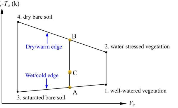
and regional scales. To overcome the di_fficulty of measuring foliage temperature in partially vegetated fields, Moran et al. (1994) proposed to use the shape of trapezoid to depict the relationship between the surface temperature and air temperature difference (Ts−Ta) vs. the fractional vegetation cover (Vc, ranging from 0 for bare soil to 1 for

full-cover vegetation) (Fig. 1), so as to combine spectral vegetation indices with composite 10

surface temperature measurements to allow application of the CWSI theory to partially vegetated fields without a priori knowledge of the percent vegetation cover. Based on the trapezoid assumption and the CWSI theory, Moran et al. (1994) introduced the Water Deficit Index (WDI) for evaluating field evapotranspiration rates and relative field water deficit for both full-cover and partially vegetated sites. For a given pixel with 15

measured surface temperature and air temperature difference, i.e., (Ts−Ta)r, WDI is

defined as:

WDI = (Ts − Ta)min − (Ts − Ta)r

(Ts −Ta)min − (Ts − Ta)max

(1)

whereT_a is air temperature; T_s is surface temperature; the subscripts min, max, and r refer to minimum, maximum, and measured values, respectively; and the minimum 20

and maximum values of (Ts−Ta) are interpolated linearly on the cold edge and warm

edge of the (T_s−T_a)∼V_ctrapezoid for the specificV_cvalue of the pixel. Graphically, WDI

(5)

HESSD

7, 8703–8740, 2010

W. Wang et al.

Title Page

Tables Figures

◭ ◮

Back Close

Full Screen / Esc

Discussion

P

a

per

|

Dis

cussion

P

a

per

|

Discussion

P

a

per

|

Discussio

n

P

a

per

|

2.2 Calculation of vertices of the(T_s−T_a₎∼V_c _{trapezoid and its simplification:}

theT_s∼VI trapezoid

The theoretical basis of (Ts−Ta)∼Vctrapezoid is the energy balance equation, i.e.,

Rn = G + H + λ E (2)

where,Rn is the net radiant heat flux density (W m

−2

), G is the soil heat flux density 5

(W m−2),H is the sensible heat flux density (W m−2), andλE is the latent heat flux to the air (W m−2) andλthe heat of vaporization (kJ/kg).

In their simplest forms,H andλE can be expressed as:

H = Cv (Ts −Ta)/ra (3)

λ E =

∆ (Rn − G) + Cv(VPD)/ra

/

∆ + γ 1 + rc/ra

(4) 10

where

– TsandTaare the land-surface and air temperature (K), respectively;

– C_v is the volumetric heat capacity of air (1295.16 J K−1m−3);

– VPD (vapor pressure deficit of the air) (hPa) is calculated as a di_fference be-tween saturation vapour pressurees and actual vapour pressureea (hPa), given

15

by (WMO, 2008)

e_S=6.112exp 17.62T ′ a

T′

a+243.12

!

(T_a′ is the air temperature in◦

C, T_a′=T_a−273.15)

ea=µes, (µ is observed relative humidity)

(6)

HESSD

7, 8703–8740, 2010

W. Wang et al.

Title Page

Tables Figures

◭ ◮

Back Close

Full Screen / Esc

Discussion

P

a

per

|

Dis

cussion

P

a

per

|

Discussion

P

a

per

|

Discussio

n

P

a

per

|

– ∆is the slope of the curve of saturation water vapour pressure versus air temper-ature, calculated with (WMO, 2008)

∆ = 4098 · e_s/

237.3 + Ta′

2

– γthe psychrometric constant (hPa/◦C), given by (WMO, 2008)

γ = 0.646 + 0.0006T_a′ 5

– rathe aerodynamic resistance (s m

−1

);

– r_c the canopy resistance to vapor transport (s m−1);

Then, combining Eqs. (2), (3), and (4), we obtain the equation for temperature di_ff er-ence between air and land surface:

(Ts − Ta) =

ra (Rn − G)/Cv γ 1 + rc/ra

/

∆ + γ 1 + rc/ra (5)

10

−VPD/_{∆ +} γ 1 + rc/ra

As suggested by Moran et al. (1994), for the (T_s−T_a)∼V_ctrapezoid, its four vertices

cor-respond to (1) well-watered full-cover vegetation, (2) water-stressed full-cover vegeta-tion, (3) saturated bare soil, and (4) dry bare soil. Using the energy balance equations, Moran et al. computed the values of the four vertices of the trapezoid as the following: 15

(1) For full-covered and well-watered vegetation (Point 1) (Ts − Ta)1 =

ra (Rn − G)/Cv γ 1 + rcm/ra

/

∆ + γ 1 + rcm/ra (6)

−VPD/_{∆ +} γ 1 + rcm/ra

wherercmis the minimum canopy resistance, i.e., canopy resistance at potential

(7)

HESSD

7, 8703–8740, 2010

W. Wang et al.

Title Page

Tables Figures

◭ ◮

Back Close

Full Screen / Esc

Discussion

P

a

per

|

Dis

cussion

P

a

per

|

Discussion

P

a

per

|

Discussio

n

P

a

per

|

(2) For full-covered vegetation with no available water (Point 2) (Ts − Ta)2 =

ra (Rn − G)/Cv γ 1 + rcx/ra

/

∆ + γ 1 ₊ rcx/ra (7)

−VPD/∆ + γ 1 + r_cx/r_a

wherercx, is the canopy resistance associated with nearly complete stomatal closure.

(3) For saturated bare soil (Point 3), where canopy resistance (rc)=0, we have

5

(Ts − Ta)3 =

ra (Rn − G)/Cv

[γ (∆ + γ)] −VPD/(∆ + γ) (8)

(4) For dry bare soil (Point 4), whererc=∞ (analogous to complete stomatal

clo-sure), andλE=0, we have

(Ts − Ta)4 = ra (Rn − G)/Cv (9)

The (Ts−Ta)∼Vctrapezoid considers that relationship between (Ts−Ta) andVc. Now we

10

think about the issue in another way that, with a given value ofTa, howTsis related with

Vc. To analysis this Ts∼Vc relationship, we use Eq. (6)∼(9) to calculate the Ts for the

four extreme cases (or trapezoid vertices) by moveTain the equations to the right side

of the equations. At the same time, Vc is replaced by vegetation index (VI). So that,

we modify the structure of the trapezoid, obtaining a simplifiedTs∼VI trapezoid with the

15

horizontal axis as VI, and the vertical axis as the surface temperatureTs. We therefore

refer the algorithm proposed here to asTs−VI trapezoid method.

To obtain the values ofTswith Eq. (6)∼(9), we need to knowra,rc(includingrcmand

r_cx),R_n,Gfor the four vertices separately, as shown in the following section.

(8)

HESSD

7, 8703–8740, 2010

W. Wang et al.

Title Page

Tables Figures

◭ ◮

Back Close

Full Screen / Esc

Discussion

P

a

per

|

Dis

cussion

P

a

per

|

Discussion

P

a

per

|

Discussio

n

P

a

per

|

2.3 Calculation of the components in the formula for four vertices of T_s∼VI trapezoid

2.3.1 Aerodynamic resistance (r_a₎

The water vapor aerodynamic resistancer_a(s/m) can be estimated with the following equation (Brutsaert, 1982):

5

ra =

ln

z − d

z0m

− ψ_m ln

z − d

z0h

− ψ_h

/k2uz (10)

where

– zis the height (m) above the surface at whichuzandTaare measured (commonly

2 m);

– uzis wind speed (m s

−1

), which could be measured directly; 10

– d is displacement height (m), given byd=0.667h, andhis the height of vegeta-tion (Garratt, 1992), which should be given as an input.

z0m is the roughness lengths for momentum (m), given by Z0m=h/8 (Garratt,

1992). For bare soil surface, z0mis commonly taken to be 0.01 m (Shuttleworth

and Wallace, 1985). 15

– z0h is the roughness lengths for heat (m), given by

z0h = z0m/exp

K B−1 ₍₁₁₎

Here,KB−1is a dimensionless parameter. Kustas et al. (1989) showed thatKB−1 is a linear function of the product ofuandTs−Ta, given by

K B−1

= SKB · u · (Ts − Ta) (12)

(9)

HESSD

7, 8703–8740, 2010

W. Wang et al.

Title Page

Tables Figures

◭ ◮

Back Close

Full Screen / Esc

Discussion

P

a

per

|

Dis

cussion

P

a

per

|

Discussion

P

a

per

|

Discussio

n

P

a

per

|

whereSKBis an empirical coefficient, which varies somewhere between 0.05 and 0.25.

– k is the von Karman constant (k=0.41);

– ψhandψmare the stability corrections for heat and momentum (unitless). ψhand

ψmare calculated differently depend on the atmospheric stability, which could be

indicated by the Monin-Obukhov lengthL, given by 5

L = −ρ C_pu3_∗ T_a/(kgH) (13)

whereg=9.8 m/s2, k=0.41, ρ is the air density (kg m−3), Cp the air specific heat at

constant pressure (1004 J kg−1K−1),u∗=uzk/[ln(z/z0m)].

For stable situations (L >0),

ψm = −5 (z − z0m)/L

ψh = −5 (z − z0h)/L

(14) 10

For unstable conditions (L≤0),

    

ψm = 2 ln

1+x 1+x₀

+ ln

1+x2 1+x2 0

− 2 tan−1(x) + 2 tan−1 x0

ψh = 2 ln

₁

+y 1+y0

(15)

where,x=

1−16(z−d)/L1/4,x₀=1−16z_0m/L1/4,y=1−16(z−d)/L1/2,

y0=

1−16z_0h/L1/2.

2.3.2 Net radiant heat flux density (R_n₎

15

Net radiation is defined as the difference between the incoming and outgoing radiation fluxes including both long- and shortwave radiation at the surface of Earth. Net radiant heat flux density (Rn) (W m

−2

) can be expressed as:

Rn = (1 − α) Rs + εa × σ × Ta4 − εsσ Ts4 (16)

(10)

HESSD

7, 8703–8740, 2010

W. Wang et al.

Title Page

Tables Figures

◭ ◮

Back Close

Full Screen / Esc

Discussion

P

a

per

|

Dis

cussion

P

a

per

|

Discussion

P

a

per

|

Discussio

n

P

a

per

|

where

– α is surface shortwave albedo, which can be calculated as a combination of MODIS narrow band spectral reflectance values (α1∼α7) (Liang et al., 1999),

given by

α = 0.3973α1 + 0.23821α2 + 0.3489α3 + 0.265α4 + 0.1604α5 − 0.0138α6

5

+0.0682α7 + 0.0036

– Rs is solar radiation, estimated jointly by solar constant, solar inclination angle,

geographical location and time of year, atmospheric transmissivity, ground eleva-tion, etc. The basic formula for estimatingR_s is (Zillman, 1972):

Rs =

S0 cos 2

θ

1.085 cos θ + e0 (2.7 + cos θ) × 10−3 + 0.1

10

whereS0is the solar constant at the atmospheric top (1367 w/m 2

), θthe solar zenith angle, e0 is the vapor pressure. In consideration of the effects of topography on the

incident short-wave radiation (Rs), the solar zenith angle (θ) is corrected using digital

elevation model (DEM) data (Duffie and Beckman, 1991) with the following formula: cosθ = sin (δ) sin (ϕ) cos (s) − sin (δ) cos (ϕ) sin (s) cos (r)

15

+cos (δ) cos (ϕ) cos (s) cos (ω) + cos (δ) sin (ϕ) sin (s) cos (r) cos (ω)

+cos (δ) sin (γ) sin (s) sin (ω)

where φ is the latitude (positive in the north hemisphere); s is the slope, and r is the slope orientation, both derived from DEM;δ is solar declination, and ωsolar hour angle, given by

20

(11)

HESSD

7, 8703–8740, 2010

W. Wang et al.

Title Page

Tables Figures

◭ ◮

Back Close

Full Screen / Esc

Discussion

P

a

per

|

Dis

cussion

P

a

per

|

Discussion

P

a

per

|

Discussio

n

P

a

per

|

ω = π

12 (t − 12)

where DOY is the day of year, andt is the time when the satellite TERRA pass over the region.

– εais the atmospheric emissivity estimated as a function of vapor pressure, given

by Iziomon et al. (2003) 5

εa = 1 − 0.35 × exp −10 × ea/Ta

– εs is surface emissivity often evaluated as a function of NDVI. For

in-stance, εs could be predicted for the 8–14 µm spectral range from NDVI using

εs=1.009+0.047 Ln (EVI) (Bastiaanssen et al., 1998). Among MODIS Land

Sur-face Temperature and Emissivity products (MOD11), there are emissivity products 10

for band 31 and 32, i.e.ε31 andε32. In the present study, we take the average of

the two products to get surface emissivity, namely,εs=(ε31+ε32)/2.

In our algorithm,Rnis not directly solved with the Eq. (16), becauseTsis considered as

an unknown variable. Instead, we replace the termRnin Eq. (6)∼(9) with the Eq. (10)

respectively, so that we get four quartic equations for Ts at four vertices separately.

15

Then the quartic equations are solved with the iterative algorithm which is shown later in Sect. 2.4 and Fig. 2, by doing so, all the values ofTsfor the four vertices are obtained.

2.3.3 Soil heat flux densityG

Gis normally considered to be linearly related toRn. Several studies have shown that

the value ofG/R_ntypically ranges between 0.4 for bare soil and 0.05 for full vegetation 20

cover (Choudhury et al., 1987). Idso et al. (1975) conducted some experiments inves-tigating the impacts of water content on the net radiation∼soil heat flux relationship over bare soil surface, and showed that G/Rn ranges from 0.2 for wet bare soil to 0.5 for dry bare soil.

(12)

HESSD

7, 8703–8740, 2010

W. Wang et al.

Title Page

Tables Figures

◭ ◮

Back Close

Full Screen / Esc

Discussion

P

a

per

|

Dis

cussion

P

a

per

|

Discussion

P

a

per

|

Discussio

n

P

a

per

|

2.3.4 Canopy resistance (r c)

Canopy resistance (rc), including rcm and rcx that refer to the minimum and maxium

canopy resistance respectively, should be calculated for Point 1 and Point 2. According to Moran et al. (1994), rcm in Eq. (6) is calculated with rsm/LAI (LAI is the leaf area

index,rsmis minimum stomatal resistance). rcx in Eq. (7) is calculated withrsx/LAI (rsx

5

is maximum stomatal resistance).

Values of minimum and maximum stomatal resistance (rsmandrsx, respectively) are

published for many agricultural crops under a variety of atmospheric conditions. Moran et al. (1994) suggested that, if values are not available, reasonable values ofr_sm=25– 100 s/m and rsx=1000–1500 s/m will not result in appreciable error, we set rsm=25

10

and rsx=1500. Because LAI are mostly less than 8 (Scurlock et al., 2001), we set

LAI=8. Therefore, we havercm=3.125 andrcx=187.5.

2.4 Iterative procedure for calculatingT_s

Values ofTsfor the four vertices are obtained by an iterative procedure for each pixel.

An initial value ofrais estimated by ignoring the two stability corrections, i.e., ψh and

15

ψm. With the initial ra, initial values of Ts are obtained with Eq. (6)∼(9) for the four

vertices. Then the iterative procedure is proceeded by iteratively changingH,KB−1,ra,

and in consequence,Ts, until the value ofTsis table (i.e., the change of Tsis less than

0.1 k, and the change ofr_a is less than 0.1 s/m). Normally, it takes 5 to 10 iterations. While Ts is derived,Rn,G,H, andrafor each vertex are obtained as well.

20

(13)

HESSD

7, 8703–8740, 2010

W. Wang et al.

Title Page

Tables Figures

◭ ◮

Back Close

Full Screen / Esc

Discussion

P

a

per

|

Dis

cussion

P

a

per

|

Discussion

P

a

per

|

Discussio

n

P

a

per

|

3 Case study area and data used

3.1 The Walnut Gulch Experimental Watershed

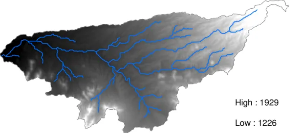
Data of the Walnut Gulch Experimental Watershed (WGEW) was used in the present study. The WGEW is defined as the upper 148 km2 of the Walnut Gulch drainage basin in an alluvial fan portion of the San Pedro catchment in southeastern Arizona 5

(Fig. 3). It was developed as a research facility by the United States Department of Agriculture (USDA) in the mid-1950s. This rangeland region receives 250–500 mm of precipitation annually, with about two-thirds of it as convective precipitation during a summer monsoon season. The potential evapotranspiration is approximately ten times annual rainfall. The runoffin the ephemeral streams is of short duration and is 10

typically near critical depth. The topography can be described as gently rolling hills incised by steep drainage channels which are more pronounced at the eastern end of the catchment near the Dragoon Mountains. Soil types range from clays and silts to well-cemented boulder conglomerates, with the surface (0–5 cm) soil textures being gravelly and sandy loams containing, on average, 30% rock and little organic matter 15

(Renard et al., 1993). The mixed grass-brush rangeland vegetation ranges from 20 to 60% in coverage. Grasses primarily cover the eastern half of the catchment, while the western half is bush-dominated.

3.2 MODIS data and ground observational data used

The moderate resolution imaging spectroradiometer (MODIS) instrument is very popu-20

lar for monitoring soil moisture because of its high spectral (36 bands) resolution, mod-erate spatial (250–1000 m) resolution, and various products for land surface properties. All standard MODIS data products are freely available at NASA Land Processes Dis-tributed Active Archive Center (URL: https://lpdaac.usgs.gov/lpdaac/). MODIS prod-ucts used in the present study include: MOD09A1 land surface albedo data, MOD11A1 25

(14)

HESSD

7, 8703–8740, 2010

W. Wang et al.

Title Page

Tables Figures

◭ ◮

Back Close

Full Screen / Esc

Discussion

P

a

per

|

Dis

cussion

P

a

per

|

Discussion

P

a

per

|

Discussio

n

P

a

per

|

we used here are listed in Table 1. We selected MODIS data of ten cloud-free days approximately evenly distributed in the period from January to December 2004. All the MODIS data are resampled to 500 m resolution.

Meteorological data required here include air temperature Ta, relative humidity µ,

and wind velocityu, observed approximately at the time (11:00 a.m.) when the satellite 5

Terra passes over the WGEW region. TheTa, relative humidity µ, and wind velocityu,

are observed at three sites. We take the average of the observations at three sites for µ andu. Observations of Ta are pre-processed, which will be discussed in Sect. 4.3.

To evaluate the soil moisture estimation results, soil moisture observations at 16 sites and precipitation data at 87 sites are used. The locations of the 3 meteorological ob-10

servation sites, 16 soil moisture observation sites and 87 rain gauging sites are plotted in Fig. 4. Because some gauging sites are located on the edge of the watershed, to include the observations at these sites for evaluation, our study area is slightly larger than the WGEW watershed.

In addition, SRTM digital elevation model (DEM) data and land cover data are used. 15

All the ground data are obtained from the website of United States Department of Agriculture (USDA) Southwest Watershed Research Center (URL: http://www.tucson. ars.ag.gov/dap/).

4 Data pre-processing

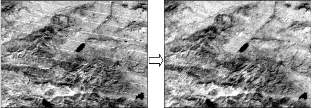
4.1 Destriping for MODDIS albedo data (MOD09A1)

20

(15)

HESSD

7, 8703–8740, 2010

W. Wang et al.

Title Page

Tables Figures

◭ ◮

Back Close

Full Screen / Esc

Discussion

P

a

per

|

Dis

cussion

P

a

per

|

Discussion

P

a

per

|

Discussio

n

P

a

per

|

The strips in Band 5 data mostly are lines of one pixel in width, which are distinguish-able from neighbouring pixels. To identify the strips, we firstly define the following two convolution kernels:

k1 =

 

0−1 0 0 1 0 0 0 0



 k2 =  

0 0 0 0 1 0 0−1 0

 

Then, we calculateKK₌convol (D,k1)×convol (D,k2), where convol(•) is the

convo-5

lution filtering function in IDL , andDis the data to be processed. A pixel in a strip is identified if KK>0.001 for this pixel. For bad pixels, linear interpolation is applied to replace the bad values using the values of upside and downside neighboring pixels.

Besides the strips of one pixel width, there are also some strips with two pixels in width resulted from the process of projection conversion in Band 5 of MOD09A1 albedo 10

product. Considering that the pixels in strips have normally higher values than normal, we identify pixels with values larger than 0.35 as “bad” pixels. Then we interpolate the bad pixels with neighbouring “good” pixels with the method of Delaunay triangle (using the program DEM BAD DATA DOIT in IDL). In the same way, pixels with value of 0 are also treated.

15

With the above two procedures, the quality of Band 5 albedo product was significantly improved (see Fig. 5).

4.2 Denosing the MOD13A1 vegetation index data

When observing the land surface, MODIS is inevitably impacted by the variation of satellite orbital position, cloud coverage and other atmospheric e_ffects. Although sev-20

eral methods (such as Maximum Value Composites or Constrained View Maximum Value Composite) have been applied to reduce the noise impacts the MODIS NDVI/EVI products, quite amount of noise still exist in the VI dataset, and filtering is still necessary when using them for constructingTs∼VI space.

(16)

HESSD

7, 8703–8740, 2010

W. Wang et al.

Title Page

Tables Figures

◭ ◮

Back Close

Full Screen / Esc

Discussion

P

a

per

|

Dis

cussion

P

a

per

|

Discussion

P

a

per

|

Discussio

n

P

a

per

|

Many methods are available to denoise the MODIS NDVI/EVI data. Jennifer (2009) compared several methods, and found that the asymmetric Gaussian, Double logistic, and 4253H twice filter perform very well in general. Therefore, one of them, i.e., 4253H twice filter (Velleman, 1980) was adopted here. The 4253H twice filter applies a series of running medians of varying window size and a weighted average filter (e.g., Hanning 5

filter), with re-roughing, to the EVI time series.

To perform the denoising process, a series of continuous EVI data over one year are required. Therefore, before we use the MODIS data selected for 10 dates, we used 25 consecutive 16-day composite EVI data (the last 16-day composite data in 2003, all 23 16-day composite EVI data in 2004, together with the first 16-day composite data 10

in 2005) to conduct the denoising procedure. The e_ffects of denoising for two randomly selected pixels are shown in Fig. 6, from which we see that, both low values and high values are smoothed.

4.3 Topographic correction of air temperature

With methods of estimating soil moisture using thermal satellite images, often both 15

land surface temperature and ground-based air temperature observations are needed. When applying such methods to mountainous regions, terrain effects have to be taken into account because terrain would significantly a_ffect both land surface temperature and air temperature. To avoid the problem of steeply sloping terrain, some authors just eliminated those pixels in mountainous part (e.g., Carlson et al., 1994), while in some 20

other cases, land surface temperature was corrected (e.g., Hassan et al., 2007). In the present study, we go the opposite way, i.e., instead of correct land surface temperature, we correct the air temperature.

To make a successful air temperature interpolation, many factors should be taken into account, such as the difference in elevation between grid points and monitoring sta-25

(17)

HESSD

7, 8703–8740, 2010

W. Wang et al.

Title Page

Tables Figures

◭ ◮

Back Close

Full Screen / Esc

Discussion

P

a

per

|

Dis

cussion

P

a

per

|

Discussion

P

a

per

|

Discussio

n

P

a

per

|

to calculate daytime temperature at different altitudes within a valley. Based on that, Bellasio et al. (2005) proposed a simplified equation in the form of

T_i = Tb − β zp − z0

+ C S_i −1/S_i 1 −LAI_i/LAImax

(17) whereT_i is the unknown atmospheric temperature (K) at a z_i altitude (m), Tb is the

measured atmospheric temperature (K) at azbaltitude (m),βis the vertical

tempera-5

ture gradient (K m−1),Cis a constant, LAImaxand LAIi are, respectively, maximum leaf

area index (LAI) and its value atz_i, andS_i is the ratio between direct shortwave radia-tion on the actual surface (with its slope and aspect) and direct shortwave radiaradia-tion on a horizontal free surface.

The above equation did not consider the impacts of wind. But according to the re-10

search of MccuTchan and Fox (1986), for their study area (an isolated, conical moun-tain with elevation ranging from 2743 to 3324 m), wind speeds greater than 5 ms−1 negate any slope, elevation or aspect differences present at low wind speed. We ap-proximate this wind effect with a coefficiente−u/3

(uis the wind speed), in sequence, obtain a modified equation of Eq. (X) as

15

T_i = Tb − β (zi − z0) + C

−u/3

e Si − 1/Si

1 − LAI_i/LAImax

(18) Therefore, when there are air temperature observations at several sites, we can con-duct air temperature correction in the following three steps:

(1) Correct the observations to a flat plane at a base level

All the temperature data are corrected to a flat plane at a base level (the lowest el-20

evation z0 of the observation sites), considering the effects of not only the elevation

difference, but also the effects of wind, slope, and aspect. This is basically a reverse correction of Eq. (X), i.e.,

T_a(i_,)_b = T_a(i) + β (z_i − z₀) − C−_eu/3 S_i − 1/S_i 1 − LAI_i/LAImax

(19)

(18)

HESSD

7, 8703–8740, 2010

W. Wang et al.

Title Page

Tables Figures

◭ ◮

Back Close

Full Screen / Esc

Discussion

P

a

per

|

Dis

cussion

P

a

per

|

Discussion

P

a

per

|

Discussio

n

P

a

per

|

whereT_a(i_,)_bis the temperature observation corrected to the base level at sitei,βis the temperature lapse rate (◦C/m),z_i is the elevation of sitei, andz0is the elevation of the

base level (m).

(2) Interpolate temperature for each pixelpusing observations on the flat plane at the base level

5

Use the corrected air temperature observationsT_a(i_,)_bto interpolate the air temperature for all pixels with a spatial interpolation method (e.g., the inverse distance weighting interpolation method) to get interpolated air temperatureT_ap_,_Ifor each pixelpon the flat plane at the base level.

(3) Topographic correction for each pixelpto its real position using Eq. (18), whereTb

10

is replaced byT_ap_,_I. Here we set LAImax=10,C=2 andβ=0.0065.

5 Application ofT

s−VI trapezoid method to WGEW

5.1 ConstructT_s−VI trapezoids

Reasonable shape of trapezoid is the essence of all the algorithms based on theTs-VI

relationship for estimating soil moisture. When construct with the algorithm described 15

in Sect. 2, two parameters, i.e.,SKB andG/Rn, are set by trial and error process. For

the case study area WGEW, we setSKB to be 0.1 for both vegetated points (point 1

and 2) and bare soil points (point 3 and 4),G/Rnto be 0.3 for wet bare soil, 0.4 for dry

bare soil, and 0.05 for full vegetation surface.

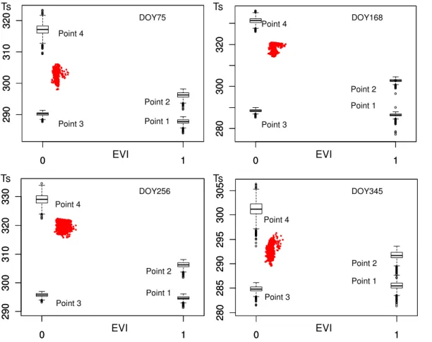
To show the effectiveness of the calculation for the values ofTs of four vertices, we

20

plot the four vertices of the trapezoids constructed for all the pixels of the WGEW region in four days in four seasons in Fig. 7. All the estimatedT_sat each point are plotted in the form of box-and-whisker plot. The data points (solid dots) ofTsvs. EVI are also plotted

in the map. From Fig. 7, we see that the constructed trapezoids well characterize the Ts-EVI space, and basically all the Ts-EVI data points are set in the envelope of the

25

(19)

HESSD

7, 8703–8740, 2010

W. Wang et al.

Title Page

Tables Figures

◭ ◮

Back Close

Full Screen / Esc

Discussion

P

a

per

|

Dis

cussion

P

a

per

|

Discussion

P

a

per

|

Discussio

n

P

a

per

|

5.2 Calculation of WDI

Based on the constructedTs-VI trapezoid for each pixel, using the MODIS Ts and EVI

data, we calculate the WDI for each pixelp,

WDI(p)=

T_S(p) − T_S(p)

,min

T_S(p)_,_min − T_S(p)

,max

(20)

whereTs is surface temperature obtained from MODIS; the subscripts min, max, and

5

r refer to minimum, maximum, and measured values, respectively; and the minimum and maximum values ofTs are interpolated linearly on the dry edge and wet edge of

theTs∼VI trapezoid for the specific VI value of the pixel.

5.3 Comparison with soil moisture observation and precipitation

Using the surface soil moisture observations at 16 sites, we evaluate WDI estimates 10

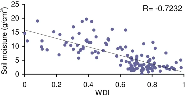
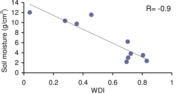
in several ways: (1) compared separate WDI estimates with ground observations of all 10 dates (Fig. 8); (2) compare the average of WDI estimates with the average ground observations of 10 dates (Fig. 9); (3) compare the WDI estimates with ground obser-vations of each date separately (Table 2).

From the scatter plot of WDI vs. observation in Fig. 8, we see that from the per-15

spective of a whole year, WDI estimates derived with theTs−VI trapezoid method has

a negative correlation (correlation coefficientR=−0.7232) with surface soil moisture,

which indicates that WDI estimates can be used to detect the temporal variation in soil moisture. Especially on the scale of the watershed, the average WDI is strongly nega-tively related (correlation coefficientR=−0.9) to the average soil moisture observation,

20

as shown in Fig. 9. Although this is not a high correlation, considering that soil moisture in dry environment, such as in semi-arid area, exhibits high spatial variability and po-tentially rapid rates of temporal change in moisture conditions, the result is reasonably good.

(20)

HESSD

7, 8703–8740, 2010

W. Wang et al.

Title Page

Tables Figures

◭ ◮

Back Close

Full Screen / Esc

Discussion

P

a

per

|

Dis

cussion

P

a

per

|

Discussion

P

a

per

|

Discussio

n

P

a

per

|

The comparison between the WDI estimates with ground observations of each date (Table 2) shows that, there is basically no correlation between WDI estimates and sur-face soil moisture observations. This is partly because of the scale effect, i.e., point soil moisture observations are essentially different from grid averaged soil moisture es-timates due to sub-grid variability, partly because of the poor capability of using WDI 5

to detect the variation in soil moisture with low spatial variability. Similar phenom-ena have been observed by some other researchers as well. For instance, Pellenq et al. (2003) noticed that the point-to-point comparison between observations and simu-lations shows a poor correlation, but a good correlation is obtained when averaging the simulated and observed soil moisture over a length of 100 m. Comparing the distribu-10

tion of soil moisture observations over the year with that observed instantaneously, we see that the coefficient of variation (CV) for all soil moisture observations at 16 sites in 10 days over a year is 0.771, much larger than the CV for observed soil in each day (ranging from 0.336 to 0.702, with a mean value of 0.528). In consequence, we can use WDI to detect the temporal variation in soil moisture, but it is hard to detect spatial 15

variation in each day, especially for a small watershed with low spatial soil moisture variability.

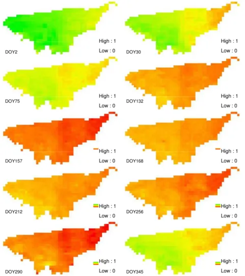
Despite of the poor performance for characterizing the spatial variability of soil mois-ture with WDI, by a visual inspection of the WDI maps of the WGEW region of the 10 dates in Fig. 10, we can still see a clear spatial pattern of soil moisture distribution, 20

which indicates that, to some extent, soil moisture variability could be depicted by WDI maps.

We analyzed the impacts of precipitation on soil moisture by calculating the correla-tion between WDI and antecedent precipitacorrela-tion (AP) of different number of days, and between soil moisture observation and AP of different number of days. The results are 25

(21)

HESSD

7, 8703–8740, 2010

W. Wang et al.

Title Page

Tables Figures

◭ ◮

Back Close

Full Screen / Esc

Discussion

P

a

per

|

Dis

cussion

P

a

per

|

Discussion

P

a

per

|

Discussio

n

P

a

per

|

of soil moisture (either reflected by ground observations, or by WDI estimates) is sig-nificantly dominated by precipitation process.

6 Conclusions

Considerable efforts have been put on using the relationship between soil moisture and index values derived from surface temperature-vegetation index (Ts∼VI) space, which

5

use optical and thermal RS data as input, to estimate soil moisture. In the present study, we simplified the trapezoidal relationship between the surface temperature and air temperature di_fference (Ts−Ta) vs. the fractional vegetation cover, which is proposed

by Moran et al. (1994), to aTs∼VI trapezoid. The trapezoid is constructed separately

for each pixel (grid). An iterative algorithm is proposed to estimate the vertices of 10

theTs∼VI trapezoid theoretically. Then water deficit index (WDI) which is calculated

based on theTs∼VI trapezoid is calculated for each grid using MODIS remotely sensed

measurements of surface temperature and enhanced vegetation index (EVI). In the process of construct theTs∼VI trapezoid, a data pre-processing procedure, including

de-striping bad pixels, eliminating the noise contamination in EVI data, and, especially 15

correcting the topographic effects for air temperature data, is conducted.

Using satellite-based MODIS data (land surface temperature data, EVI, etc.), and ground-based on-site soil moisture data and meteorological data (air tempera-ture, relative humidity, and wind velocity) for the Walnut Gulch Experimental Water-shed (WGEW) in Arizona, USA, the capability of using WDI to estimate soil moisture is 20

evaluated using (1) a soil moisture observations and (2) antecedent precipitation. The result shows that, Ts∼VI trapezoid based WDI can well capture temporal variation in

surface soil moisture, but the capability of detecting spatial variation is poor for such a semi-arid region as WGEW.

Acknowledgements. We are very grateful to USDA Southwest Watershed Research Center 25

for providing observation data of the Walnut Gulch Experimental Watershed. The financial supports from China Postdoctoral Science Foundation (20080431062), the National Science Foundation of China (40771039) and the 111 Project (B08048) are gratefully acknowledged.

(22)

HESSD

7, 8703–8740, 2010

W. Wang et al.

Title Page

Tables Figures

◭ ◮

Back Close

Full Screen / Esc

Discussion

P

a

per

|

Dis

cussion

P

a

per

|

Discussion

P

a

per

|

Discussio

n

P

a

per

|

References

Bastiaanssen, W. G. M. and Menentia, M.: A remote sensing surface energy balance algorithm for land (SEBAL) 1. Formulation, J. Hydrol., 212, 198–212, 1998.

Bellasio1, R., Maffeis, G., and Scire, J. S.: Algorithms to Account for Topographic Shading Effects and Surface Temperature Dependence on Terrain Elevation in Diagnostic Meteoro-5

logical Models, Bound.-Lay. Meteorol., 114, 595–614, 2005.

Brutsaert, W.: Evaporation into the Atmosphere: Theory, History and Applications, D. Reidel, Dordrecht, The Netherlands, 299 pp., 1982.

Carlson, T. N., Gillies, R. R., and Perry, E. M.: A method to make use of thermal infrared tem-perature and NDVI measurements to infer surface soil water content and fractional vegetation 10

cover, Remote Sens. Rev., 9, 161–173, 1994.

Choudhury, B. J., Idso, S. B., and Reginato, J. R.: Analysis of an empirical model for soil heat flux under a growing wheat crop for estimating evaporation by an infrared-temperature based energy balance equation, Agr. Forest Meteorol., 39, 283–297, 1987.

Duffie, J. A. and Beckman, W. A.: Solar engineering of thermal process, 2nd edition, John 15

Wiley and Sons, New York, USA, 1991.

Garratt, J.: The Atmospheric Boundary Layer, Cambridge University Press, New York, USA, 316 pp., 1992.

Gillies, R. R., Carlson, T. N., Cui, J., Kustas, W. P., and Humes, K. S.: A verification of the “triangle” method for obtaining surface soil water content and energy fluxes from remote 20

measurements of the Normalized Difference Vegetation Index (NDVI) and surface radiant temperature, Int. J. Remote Sens.,18, 3145–3166, 1997.

Goward, S. N., Cruickhanks, G. D., and Hope, A. S.: Observed relation between thermal emis-sion and reflected spectral radiance of a complex vegetated landscape, Remote Sens. Envi-ron., 18, 137–146, 1985.

25

Hassan, Q. K., Bourque, C. P. A., Meng, F. R., and Cox, R. M.: A wetness index using terrain-corrected surface temperature and normalized difference vegetation index derived from stan-dard MODIS products: An evaluation of its use in a humid forest-dominated region of eastern Canada, Sensors, 7, 2028–2048, 2007.

Ian, D. M. , Norton, T. W., and Williams, J. E.: Modelling environmental heterogeneity in forested 30

(23)

HESSD

7, 8703–8740, 2010

W. Wang et al.

Title Page

Tables Figures

◭ ◮

Back Close

Full Screen / Esc

Discussion

P

a

per

|

Dis

cussion

P

a

per

|

Discussion

P

a

per

|

Discussio

n

P

a

per

|

Idso, S. B., Aase, J. K., and Jackson, R. D.: Net radiation – Soil heat flux relations as influenced by soil water content variations, Bound.-Lay. Meteorol., 9, 113–122, 1975.

Idso, S. B., Jackson, R. D., Pinter Jr., P. J., Reginato, R. J., and Hatfield, J. L.: Normalizing the stress-degree-day parameter for environmental variability, Agr. Meteorol., 24, 45–55, 1981. Iziomon, M. G., Mayer, H., and Matzarakis, A.: Downward atmospheric longwave irradiance 5

under clear and cloudy skies: Measurement and parameterization, J. Atmos. Sol.-Terr. Phy., 65, 1107–1116, 2003.

Jackson, R. D., Idso, S. B., Reginato, R. J., and Pinter, P. J.: Canopy temperature as a crop water stress indicator, Water Resour. Res., 17, 1133–1138, 1981.

Jennifer, N. H. and McDermid, G. J.: Noise reduction of NDVI time series: An empirical com-10

parison of selected techniques, Remote Sens. Environ., 113, 248–258, 2009.

Kustas, W. P., Choudhury, B. J., Moran, M. S., Reginato, R. J., Jackson, R. D., Gay, L. W., and Weaver, H. L.: Determination of sensible heat flux over sparse canopy using thermal infrared data, Agr Forest Meteorol., 44, 197–216, 1989.

Liang, S.: Retrieval of Land Surface Albedo from Satellite Observations: A Simulation Study[J], 15

J. Appl. Meteorol., 38, 712–725, 1999.

Margulis, S. A., Kim, J., and Hogue, T.: A Comparison of the Triangle Retrieval and Varia-tional Data Assimilation Methods for Surface Turbulent Flux Estimation, J. Hydrometeorol., 6, 1063–1072, 2005.

McCutchan, M. H. and Fox, D. G.: Effect of Elevation and Aspect on Wind,Temperature and 20

Humidity, J. Clim. Appl. Meteorol., 25(12), 1996–2013, 1986.

Moran, M. S., Clarke, T. R., Inoue, Y., and Vidal, A.: Estimating crop water deficit using the rela-tion between surface air temperature and spectral vegetarela-tion index, Remote Sens. Environ., 49, 246–263, 1994.

Nemani, R. R. and Running, S. W.: Estimation of regional surface resistance to evapotranspi-25

ration from NDVI and thermal IR AVHRR data, J. Appl. Meteorol., 28, 276–284, 1989. Nemani, R. R., Pierce, L., Running, S. W., and Goward, S.: Developing satellite-derived

esti-mates of surface moisture status, J. Appl. Meteorol., 32, 548–557, 1993.

Pellenq, J., Kalma, J., Boulet, G., Saulnier, G. M., Wooldridge, S., Kerr, Y., and Chehbouni, A.: A disaggregation scheme for soil moisture based on topography and soil depth, J. Hydrol. 30

,276, 112–127, 2003.

Price, J. C.: Using spatial context in satellite data to infer regional scale evapotranspiration [J], IEEE T. Geosci. Remote, 28, 940–948, 1990.

(24)

HESSD

7, 8703–8740, 2010

W. Wang et al.

Title Page

Tables Figures

◭ ◮

Back Close

Full Screen / Esc

Discussion

P

a

per

|

Dis

cussion

P

a

per

|

Discussion

P

a

per

|

Discussio

n

P

a

per

|

Renard, K. G., Lane, L. J., Simanton, J. R., Emmerich, W. E., Stone, J. J., Weltz, M. A., Goodrich, D. C., and Yakowitz, D. S.: Agricultural impacts in an arid environment: Walnut Gulch case study, Hydrol. Sci. Tech., 9(1–4), 145–190, 1993.

Sandholt, I., Rasmussen, K., and Andersen, J.: A Simple Interpretation of the Surface Tem-perature/Vegetation Index Space for Assessment of Surface Moisture Status, Remote Sens. 5

Environ., 79(2), 213–224, 2002 .

Scurlock, J. M. O., Asner, G. P., and Gower, S. T.: Global Leaf Area Index Data from Field Mea-surements, 1932–2000, Data set, available on-line at http://www.daac.ornl.gov from the Oak Ridge National Laboratory Distributed Active Archive Center, last access: 1 August 2010, Oak Ridge, Tennessee, USA, 2001.

10

Shuttleworth, W. and Wallace, J.: Evaporation from Sparse Crops – An Energy Combination Theory, Q. J. Roy. Meteor. Soc., 111, 839–855, 1985.

Skirvin, S., Kidwell, M., Biedenbender, S., Henley, J. P., King, D., Collins, C. H., Moran, S., and Weltz, M.: Vegetation data, Walnut Gulch Experimental Watershed, Arizona, United States, Water Resour. Res., 44, W05S08, doi:10.1029/2006WR005724, 2008.

15

Smith, R. C. G. and Choudhury, B. J.: Analysis of normalized difference and surface temper-ature observations over southeastern Australia, Int. J. Remote Sens., 12(10), 2021–2044, 1991.

Tang, R., Li, Z.-L., and Tang, B.: An application of theT_sVI triangle method with enhanced edges determination for evapotranspiration estimation from MODIS data in arid and semi-20

arid regions: Implementation and validation, Remote Sens. Environ., 114, 540-551, 2010. Velleman, P.: Definition and comparison of robust nonlinear data smoothing algorithms, J. Am.

Stat. Assoc., 75, 609–615, 1980.

World Meteorological Organization (WMO): Guide to Meteorological Instruments and Methods of Observation, WMO-No. 8 (CIMO Guide), Geneva, 2008.

25

(25)

HESSD

7, 8703–8740, 2010

W. Wang et al.

Title Page

Tables Figures

◭ ◮

Back Close

Full Screen / Esc

Discussion

P

a

per

|

Dis

cussion

P

a

per

|

Discussion

P

a

per

|

Discussio

n

P

a

per

|

Table 1.MODIS data used in the present study.

Product ID Contents Spatial Temporal

resolution resolution

MO03 Geolocation Data Set 1 km daily

MOD09A1 Surface Reflectance 500 m 8 days

MOD11A1 Surface Temperature and Emissivity 1 km daily MCD12Q1 Land Cover and Vegetation Dynamics 500 m Yearly

MOD13A1 Vegetation Indices 250 m 8 days

MOD15A2 Leaf Area Index 1 km 8 days

(26)

HESSD

7, 8703–8740, 2010

W. Wang et al.

Title Page

Tables Figures

◭ ◮

Back Close

Full Screen / Esc

Discussion

P

a

per

|

Dis

cussion

P

a

per

|

Discussion

P

a

per

|

Discussio

n

P

a

per

|

Table 2. Correlation coe_fficients between WDI estimates with surface soil moisture observa-tions.

DOY 345 290 256 212 168 157 132 75 30 2

(27)

HESSD

7, 8703–8740, 2010

W. Wang et al.

Title Page

Tables Figures

◭ ◮

Back Close

Full Screen / Esc

Discussion

P

a

per

|

Dis

cussion

P

a

per

|

Discussion

P

a

per

|

Discussio

n

P

a

per

|

−

=

−

λ

= + +

Ȝ

C

T

_s

_-

T

_a

_(k)

3. saturated bare soil

1. well-watered vegetation

2. water-stressed vegetation

4. dry bare soil

B

A

y

Dry/warm edge

Wet/cold edge

V

c

Fig. 1. The hypothetical trapezoidal shape based on the relation between (T_s−T_a) and the fractional vegetation cover (V_c).

(28)

HESSD

7, 8703–8740, 2010

W. Wang et al.

Title Page

Tables Figures

◭ ◮

Back Close

Full Screen / Esc

Discussion

P

a

per

|

Dis

cussion

P

a

per

|

Discussion

P

a

per

|

Discussio

n

P

a

per

|

ȥ ȥ

constructed separately for each pixel, and each trapezoid has it

Calculate initial r_a_{without considering}

ȥh and ȥm

Solve the quartic equations for Ts by replacing r_a_{in Eq. (8)~(11)}

Calculate T_s_–T_a

Calculate H with Eq. (5) for each vertex

Calculate KB-1_{with Eq. (14) and}L_{with Eq.} (15) for each vertex

Correct the value of r_a_consideringȥ_h_andȥ_m_as in Eq. (16) or (17) depending on the value of L

Output the values of R_n_{, G, H,}r_a_{, and}T_s_for each vertex

Meteorological data: Ta, u, ȝ,

MODIS data: Ts,

10 iterations

(29)

HESSD

7, 8703–8740, 2010

W. Wang et al.

Title Page

Tables Figures

◭ ◮

Back Close

Full Screen / Esc

Discussion

P

a

per

|

Dis

cussion

P

a

per

|

Discussion

P

a

per

|

Discussio

n

P

a

per

|

High : 1929

Low : 1226

Fig. 3.Digital elevation model (DEM) of Walnut Gulch Experimental.

(30)

HESSD

7, 8703–8740, 2010

W. Wang et al.

Title Page

Tables Figures

◭ ◮

Back Close

Full Screen / Esc

Discussion

P

a

per

|

Dis

cussion

P

a

per

|

Discussion

P

a

per

|

Discussio

n

P

a

per

|

ȝ

-

--

-_

_

Meteorological observation station

- Soil moisture observation site Rain gage

，

⎡

⎤

⎢

⎥

= ⎢

⎥

⎢

⎥

⎣

⎦

⎡

⎤

⎢

⎥

= ⎢

⎥

⎢

−

⎥

⎣

⎦

y

Fig. 4.Locations of ground-based observation sites in WGEW.

(31)

HESSD

7, 8703–8740, 2010

W. Wang et al.

Title Page

Tables Figures

◭ ◮

Back Close

Full Screen / Esc

Discussion

P

a

per

|

Dis

cussion

P

a

per

|

Discussion

P

a

per

|

Discussio

n

P

a

per

|

Fig. 5 Comparison of Band 5 albedo images before (left) and after destriping Fig. 5.Comparison of Band 5 albedo images before (left) and after destriping.

(32)

HESSD

7, 8703–8740, 2010

W. Wang et al.

Title Page

Tables Figures

◭ ◮

Back Close

Full Screen / Esc

Discussion

P

a

per

|

Dis

cussion

P

a

per

|

Discussion

P

a

per

|

Discussio

n

P

a

per

|

0.06 0.08 0.1 0.12 0.14 0.16 0.18

0 5 10 15 20 25

Data Order

EVI

Before Denoising After Denoising

0.1 0.15 0.2 0.25 0.3

0 5 10 15 20 25

Data Order

EVI

Before Denoising After Denoising

(33)

HESSD

7, 8703–8740, 2010

W. Wang et al.

Title Page Abstract Introduction Conclusions References Tables Figures ◭ ◮ ◭ ◮ Back Close

Full Screen / Esc

Printer-friendly Version Interactive Discussion Discussion P a per | Dis cussion P a per | Discussion P a per | Discussio n P a per | 0 1 29 0 3 00 310 3 2 0 0 1 29 0 3 00 310 3 2 0 0 1 280 300 3 20 0 1 280 300 3 20 0 1 290 300 3 10 320 330 0 1 290 300 3 10 320 330 0 1 28 0 2 85 29 0 295 30 0 3 05 0 1 28 0 2 85 29 0 295 30 0 3 05 − = − DOY345 DOY256

DOY75 DOY168

Point 2 Point 1 Point 3 Point 4 Point 2 Point 1 Point 3 Point 4 Point 2 Point 1 Point 3 Point 4 Point 2 Point 1 Point 3 Point 4 Ts Ts Ts Ts EVI EVI EVI EVI

Fig. 7.ConstructedT_s−EVI trapezoids in four dates in four different seasons.