The Analysis of the Cold Flat Rolling Process by Salf Program
Gilberto Thiago de Paula Costaa, Carlos Augusto dos Santosb*
Received: October 25, 2016; Revised: February 06, 2017; Accepted: February 18, 2017
SALF program is a Brazilian program developed to simulate the cold lat rolling process by the inite element method. The program uses the implicit and rigid-plastic approaches to perform numerical analyses. This article presents the cold lat rolling simulations performed by SALF, where the variables of rolling force, efective strain rate, and efective strain were analyzed. The simulations were chosen from the literature and involved materials such as steel and aluminum, with thicknesses of 1.0 mm and 3.0 mm, reductions of 5%, 16.67%, and 30%, and friction coeicients of 0.08, 0.1, and 0.3. The results showed that SALF describes the above variables appropriately in qualitative and quantitative terms. However, based on the research results, domestic steel industries may now use a national program to simulate the cold lat rolling process to improve their processes and products.
Keywords: Cold Flat Rolling Process; Finite Element Method; Implicit and Rigid-Plastic Approaches
* e-mail: solracbr@gmail.com
1. Introduction
The cold lat rolling process provides raw material for several industries such as electronics, appliances, and transportation. Examples of raw materials include sheets used in personal computers, appliances, cars, planes, and locomotives. It is also important to reinforce that the volume of rolled steel in Brazil reached 17.0 million tons in irst three quarters of 2015, 8.2 million tons being lat-rolled products1. Cold lat-rolled products in the same period
reached 2.0 million tons, 24.4% of lat-rolled products, and 11.8% of Q1-Q3 production1. According to the above facts,
cold lat-rolled products play a vital role in the economy. Analyses of the cold lat rolling process have been performed using one or more of following approaches: analytical, numerical, and experimental. In general, analytical studies involve applications of uniform energy, slab, or upper-bound methods2-6. These methods present limitations involving geometries of processes and descriptions of material hardening. Because of these limitations, the methods are commonly used as starting points to estimate the forming load in simple processes: upsetting, lat rolling, drawing, and extrusion. The inite element method (FEM) has been used in the majority of numerical analyses. The FEM advantage consists in describing a large number of process variables in a short time period: distribution of efective strain and stress, load and torque rolling, raw material defects, friction hill, and damage7-13. The experimental approach serves to provide real data and is fundamental to understand the process. Tests
performed either on the actual equipment, on the idealized prototypes, or in the labs furnish the experimental data14-17. In relation to analytical and numerical analyses, this approach demands more time and costs with equipment, raw material, and manual labor.
The analytical methods have remained unchanged since the Mid-20th Century. However, FEM has developed constantly, and its application enhances understanding of the lat rolling process. Improvements in measurement equipment have been the most signiicant developments in the experimental area. Based on these three considerations, traditional analytical methods continue to be used only to estimate the forming load in simple processes. FEM plays an important role because it provides an overall understanding of the process variables in a short time period. The experimental approach remains important inside analyses because its experimental data validate the FEM results.
The irst commercial FEM program, DEFORM 2D and 3D (USA), dedicated to simulate metal forming processes, appeared in 1990, following the development of automated mesh generation and workstation processing capability18.
Over time, other commercial programs have been developed, such as: FORGE (France)19, QFORM (Russia)20, MSCForge
(USA)21, ABAQUS (USA)22, and SIMUFACT (Germany)23.
The full version of these programs enables users to perform 2D or 3D simulations involving analyses of the following phenomena: mechanics (stress, strain or damage distribution), heat transfer, phase transformation, and difusion18. A basic FEM
program devoted to metal forming processes only performs mechanical analyses, speciically stress and strain evaluations. a Radioactive Waste Management Department, Brazilian Nuclear Energy Commission, Rua General
Severiano 90, Botafogo, CEP: 22290-040, Rio de Janeiro, RJ, Brazil
b Department of Mechanical Engineering, School of Engineering, Fluminense Federal University, Rua
This program works as a seed to develop more elaborate programs involving heat transfer, phase transformation, or difusion analyses because they depend on the mechanical evaluations of stress and strain.
In Brazil, the steel industries producing cold lat-rolled products still lack a national FEM program to simulate the lat rolling process. These companies use international FEM programs, such as those mentioned above. Licensing is expensive, and technical support is frequently unable to solve simulation problems. However, developing research in Brazil to create a national FEM software program is crucial. Such software will enable domestic steel industries to incorporate recent technology to improve their products and processes.
This article introduces SALF program, Sistema de Análise de Laminação a Frio, a cold lat rolling analysis system. The program is the irst Brazilian tool directed at simulating the cold lat rolling process using FEM. SALF performs simulations focused on mechanical phenomena, speciically stress and strain analyses. The second section of the article shows the mathematical theory employed to develop the software. However, this part of the article contributes to disseminate the information necessary to create FEM programs of this nature. The information will help developers design software like SALF or develop more elaborate programs that analyze other phenomena such as heat transfer, phase transformation, and difusion, thereby increasing the number of national software programs dedicated to metal forming processes. SALF development involved ideas of structured and object-oriented programming using FORTRAN 90 language. Preprocessing and post processing were developed using the oriented-object approach, while the processor used the structured approach.
2. Theoretical Approach
The program was developed based on the implicit and low formulations7, speciically adapted for the cold lat
rolling process. The following items present the key points of this development.
2.1. Basic deinitions
This part of the process involves describing the initial data to start the simulation: sheet and roll geometrical characteristics; mechanical behavior of material; friction and velocity boundary conditions; and governing equations. The universal curve deines mechanical behavior. This curve relates the efective stress to the efective strain rate. The friction model characterizes the shear stress in the surface between sheet and roll. The chosen model for this program was the constant frictional stress. The sheet and roll velocities represent the velocity conditions. The governing equations of the simulation are related in (1), respectively:
equilibrium equations, yield criteria, constitutive equations, and compatibility conditions.
( ) ( ) ( )
( )
( ) x
Y
x u
x u 0
6 2
2 3
2
1 1
’ j ij
x y y z z x
xy yz zx
ij ij
ij
j i
i j
2 2 2
2 2 2 2
2 2
2 2
2 2 v
v v v v v v
x x x
f vfv f
=
- + - + - +
+ + =
=
= +
o ro
o T Y
In (1), σ represents the stress tensor components, x characterizes the global coordinate, Y is the yield strength, ε̇ corresponds to the strain rate tensor components, is the efective strain rate, characterizes the efective stress, is the deviatoric stress tensor components, and u represents the nodal velocity.
2.2. Domain discretization
Discretization consists in dividing the interest domain (sheet or sheet/roll) in several elements to create a mesh, with shared element-sides. The node velocity in the shared element-side is the same for both elements. Figure 1 shows a mesh created for a rolling simulation.
fo
vr vl
Figure 1. Example of mesh in lat rolling.
The mesh uses four-noded and four-sided isoparametric elements, with the velocities in any element part described by
( , ) ( , ).
( , ) ( , ). ( )
u q u
u q u 2
x x
y x
p h p h
p h p h
= =
a
a
a
a
G
/
/
J
where α represents the nodal point, qαits shape function, and uxα and uyα are the nodal velocities in the global coordinates. The shape function value in any part of the element is calculated from
( , ) ( )( ) ( )
qa p h =1 14 +p pa 1+h ha 3
with the variables ξ and η representing the local coordinate system for the element.
2.3. Establishing the element equation
by internal forces, and the second, the work performed by external forces. The variables and are respectively, the efective stress and efective strain rate, both being functions of the velocity ield variable. The term Fi is the prescribed
stress on the sheet boundary, and ui represents the velocity. Equation (4) requires that the solution ield satisies the compatibility, incompressibility, and boundary conditions, in addition to providing a stationary value to the variational.
vr fo
( )
dv F u ds 4
v
i s
i r=
#
vfr ro -#
The required stationary value comes from the equation deined in (5). The second term in this equation represents the penalized form of the incompressbility11 used to remove
the incompressibility constraint in the velocity ield.
.
( )
dv K dv
F u ds 0 5
v v v v i s i
dr v df f df
d
= +
-=
r ro o o
#
#
#
In (5), K corresponds to the penalty constant. The efective strain rate and volumetric strain rate ε̇vdepend
on the strain rate tensor fo
( )
x u x
q u q 2 1 6 ij
j i i j
2 2
2 2
f = a a+ a a
a
o
/
T Ywhich assumes the matrix format
( )
.
B u 7
fo =
... ... ... ( ) y y y y B q q q q
q q q q
0 0
0 0 2
0 0 0 0
8
1 2
1
1 1 2 2
2 2 2 2 2 2 2 2 2 2 2 2 2 2 2 2 \ \ \ \ = R T SS SS SS SS SS SS SS SS SS V X WW WW WW WW WW WW WW WW WW
with B representing the strain rate matrix of the element and u representing the nodal velocity vector of the element. The components in matrix B correspond to the partial derivatives of the shape function in relation to the global coordinates. The third line in B presents zero entrances because in the width direction of cold lat rolling processes, the plain strain condition prevails. Adopting the strain rate tensor, the efective strain rate and volumetric strain rate are deined as
(u B DBuT T )2 (u PuT ) ( )9
1
2 1
fro= =
( )
P=B DBT 10
( ) D
3 2 0 0 0
0 32 0 0 0 0 32 0 0 0 0 31
11 = R T SS SS SS SS SS SS SS SS SSS V X WW WW WW WW WW WW WW WW WWW ( )
C u C u 12
v T i i
fo = =
( ) Ci=Bli+B2i+B3i 13
The solution in (5) consists in solving the non-linear equation system deined in (14), where ui represents the nodal
velocities in the x and y directions. A set of eight equations is established for each element because of the two degrees of freedom in each node.
( )
ui 0 14
d dr =
The system in (14) requires an iterative method for its solution due to its nonlinearity. The Newton-Raphson method has been the most used in metal forming simulations. The irst step of the method characterizes a linearization of (14) by Taylor expansion, which results in the following equation
The term Δuj in (15) represents the irst-order correction
of the velocities, and the others characterize integrals with the following discretized form
( )
ui u ui j uj 0 15
2 2 2
2 d
dr +# r &D =
( )
u P u dv K C C dv F N ds
u u P dv K
C C dv P u u P dv
u
16 1 1 j j i v ij j j vj i j
s ji v ij j v i v
ik k m mj 2 2 d dr f v d d d r f v f df dv v f
f
= + -= + + -p pp p p p
T
Y
#
#
#
#
#
#
with P and D deined in (10) and (11), and N described in terms of the shape functions in (17).
... ... ( ) q q q q N 0 0 0 0 17 1 1 2 2 = R T SS SS SS SS SS SS SS SS V X WW WW WW WW WW WW WW WW
2.4. Deinition and solution of the global equation
freedom with the equation variables corresponding to the nodal velocities. In (18), the k parameter deines all elements sharing the velocity ui.
along the arc of contact. Rotation of this tensor according to the speciic angle produces the normal stress component acting on the roll for each nodal point along the arc of contact. Using these stress components, the integral in (22) furnishes the roll force per unit of width
( )
ui u u u 0 18
j
i j j
j k
2 2 2
2 2 2
r r
D
+ =
T Y
/
The Gaussian Elimination method has been used to solve the linear equation system obtained from (18). The method employs the norm deined in (19) to verify the convergence of the Newton-Raphson method
( ) ( )
error uu
u u uT 12 19
# << <<
< <
D
=
with Δu characterizing the correction velocity vector and u, the vector velocity. In general, this norm should be
smaller than 5x10⁻⁵.
2.5. Geometry updating, stress tensor, and total
efective strain
The nodal velocities are updated using the vector Δu obtained from the convergence of the Newton-Raphson method. The new velocity ield enables redeining the nodal coordinates using the equations described in (20)
( )
x x u
x y u
t t
20
x y 0 0
D
D
= +
= +
where x0 and y0 represent the previous nodal coordinates,
and Δt the step time size.
Deining the stress tensor employs the ideas described in 2.1, and the equation in (21) deines how to obtain the total efective strain
( )
t 21
t t t
fr+D =fr +froD
with representing the total efective strain of previous step and the efective strain rate in the current step.
2.6. Rolling force
The stress tensor of the nodal points in contact with the roll furnishes information to obtain the rolling pressure
t
fr fo
. ( ) ( )
w
F p ds w p x 22
n n
n
=
#
=/
with wn representing the weight factor, xn characterizing
the integration point, and p(xn) representing the normal stress
in the integration point.
3. Evaluation of the Program
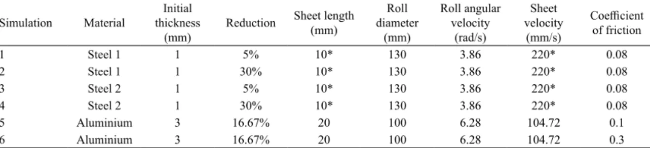
The irst evaluation step consisted of comparing force results recorded in the simulations from the literature and those obtained from SALF when repeating the simulations with the program. The chosen simulations were based on conditions representing the raw materials and thicknesses that are commonly involved in cold lat rolling, as shown in Table 1. In simulations 4 and 5, a study of the efective strain and efective strain rate was also performed. The data with an asterisk in the table were chosen from other articles due to the lack of their deinitions in the reference article.
The control data for simulations in Table 1, time per step, limiting strain rate, and penalty constant were 0.001 s, 0.01 s-1, and 10,000.00, respectively. In simulations 5 and 6, the article of reference provided the element number used in the mesh. In the other simulations, the element number followed a proportion in relation to simulations 5 and 6.
4. Results
4.1. Force results
In simulations 1 and 2 in Table 1, the article of reference used the procedure described in RAMBERG and OSGOOD25
to deine the low stress curve of the material employed in the simulations. The procedure used the Young´s modulus of the material and the stresses obtained in the strain values of 0.1% and 0.2% to describe the whole curve. Figure 2 shows the curve obtained according to the above ideas.
Considering the conditions of simulations 1 and 2, Table 2 presents the force results from the analytical methods, SALF, FEM from ESCRIBANO, et al.24, and the experimental data.
Table 1. Simulations chosen from the literature11,24.
Simulation Material
Initial thickness
(mm) Reduction
Sheet length
(mm)
Roll diameter
(mm)
Roll angular velocity
(rad/s)
Sheet velocity
(mm/s)
Coeicient of friction
1 Steel 1 1 5% 10* 130 3.86 220* 0.08
2 Steel 1 1 30% 10* 130 3.86 220* 0.08
3 Steel 2 1 5% 10* 130 3.86 220* 0.08
4 Steel 2 1 30% 10* 130 3.86 220* 0.08
5 Aluminium 3 16.67% 20 100 6.28 104.72 0.1
Figure 2. Flow stress curve used in simulations 1 and 2.
Neither SALF nor FEM from ESCRIBANO, et al.24 presented a relevant approximation between their results and the experimental data. The analytical homogeneous deformation method underestimated the experimental data while the slab method presented data close to the experimental data. All the results in Table 2 present the anticipated force behavior in relation to the reduction: the force results increased as a higher reduction was employed.
It is noteworthy that despite using the low stress curve obtained following to the procedure in RAMBERG and OSGOOD25, SALF simulation presented force values
below those in FEM from ESCRIBANO, et al.24 shown in Table 2. Because of the procedural uncertainties, a set of new simulations using SALF were performed. These simulations employed a low stress curve with a higher work hardening coeicient in relation to the curve in Figure 2. Figure 3 shows the low stress curve that produced the best force results, as explained above.
Table 3 presents the force results as in Table 2, with SALF simulations using the low stress curve of Figure 3. According to the data in Table 3, SALF presented excellent force results in relation to the experimental force values. However, these new simulations in Table 3 showed that in qualitative and quantitative terms, SALF is able to correctly describe the relation between force versus reduction.
Table 2. Force versus reduction - simulation 1: reduction of 5%; simulation 2: reduction of 30%.
Simulation Material
Homogeneous
deformation
method
Slab method SALF
FEM ESCRIBANO,
et al.24
Experimental ESCRIBANO,
et al.24
1 (N/mm) Steel - low stress by RAMBERG
and
OSGOOD25
769 1228 747 1400 1100
2 (N/mm) 2095 3307 2012 3400 3150
Table 3. Force versus reduction - simulation 3: reduction of 5%; simulation 4: reduction of 30%.
Simulation Material
Homogeneous
deformation
method
Slab method SALF
FEM ESCRIBANO,
et al.24
Experimental ESCRIBANO,
et al.24
3 (N/mm) Curve with modiied
hardening
coeicient
853 1451 1073 1400 1100
4 (N/mm) 2464 4223 3140 3400 3150
Figure 3. Flow stress curve used in simulations 3 and 4.
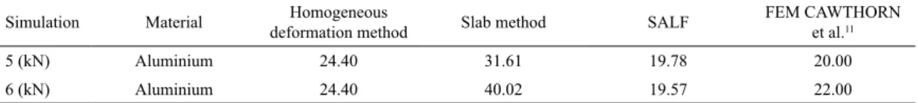
The relation between force versus friction was analyzed in simulations 5 and 6 in Table 1. The material for these simulations was aluminum with a Young´s modulus of 69.0 GPA, as described in the reference article. However, considering the size of this Young´s modulus, a low stress obtained from the literature26 was employed in SALF
simulations, shown in Figure 4. The roll and sheet velocities were provided in the reference article.
Table 4 shows strong agreement between the force results of SALF and CAWTHORN et al.11. In these
simulated conditions, the analytical results overestimated the numerical force results of SALF and CAWTHORN et al.11. A constancy of the force results with the variation of the
friction coeicient was observed in SALF and CAWTHORN et al.11. This constancy was also presented in PRAKASH,
et al.8. However, the results in this analysis demonstrated
the SALF potential in describing the relation between force and friction.
Figure 4. Flow stress curve used in simulations 5 and 6.
value at the beginning of the contact between the steel and roll. As the material is processed, the value decreases along the interface of the sheet and roll. In the literature6, the
region presenting a small value of the efective strain rate, below the interface of the sheet and roll, is called restricted low zone. Inside this zone, the material presents a small deformation, causing an excessive pressure on the central material. The excessive pressure produces the high value of the efective strain rate at the central region in igures 5 and 6. Near the end of the sheet and roll contact region, the restricted low zone disappears and the efective strain rate presents a small increase. The rate distribution in simulations 4 and 5 is similar to that observed by LIN and SHEN27 and
KOMORI28.
Table 4. Force versus friction - simulation 5: coeicient of friction of 0.1; simulation 6: coeicient of friction of 0.3.
Simulation Material deformation methodHomogeneous Slab method SALF FEM CAWTHORN et al.11
5 (kN) Aluminium 24.40 31.61 19.78 20.00
6 (kN) Aluminium 24.40 40.02 19.57 22.00
Figure 5. Efective strain rate - thickness of 1.0 mm, velocity of
250.00 mm/s and reduction of 30% (simulation 4).
Figure 6. Efective strain rate - thickness of 3.0 mm, velocity of
104.72 mm/s and reduction of 16.67% (simulation 5).
In relation to the efective strain, results in Figures 7 and 8 show an increasing strain value from the beginning of the reduction to the exit of the sheet. The higher values of efective strain after the sheet leaves the roll appear on the sheet surface and in its central region. This behavior is a consequence of the efective strain rate results: the higher values of this variable also appear on the sheet surface and in its central region. The results shown in Figures 7 and 8 are similar to those from RICHELSEN29.
Figure 7. Efective strain - thickness of 1.0 mm, velocity of 250.00
mm/s and reduction of 30% (simulation 4).
Figure 8. Efective strain rate - thickness of 3.0 mm, velocity of
104.72 mm/s and reduction of 16.67% (simulation 5).
5. Conclusions
According to the results in the above item, the SALF program permits simulating the cold lat rolling process. However, domestic steel industries now have a national tool to simulate their processes using FEM. In future SALF tests, simulating other rolling conditions using data obtained from steel industries will be vital. These new simulations will provide information about the program performance inside the whole range of conditions in the cold lat rolling process, revealing any necessary program adjustments.
The content presented in the article disseminates the knowledge necessary to develop FEM programs focused on simulating metal forming processes. However, based on this article, other national developers can create more metal forming programs, thereby increasing the number of related national software products.
Additionally, SALF is the seed program for future research simulating the lat rolling process by analyzing damage, heat transfer, and phase transformation. Including these analyses will allow SALF to be eiciently used throughout the entire universe of the lat rolling process.
6. References
1. SICETEL. Sindicato Nacional das Indústrias de Treilação e Laminação de Metais Ferrosos. Estatísticas Setoriais. Available
from: <http://www.sicetel.org.br/>. Acess in: Feb 29/02/2016. 2. Thomsen EG, Charles TY, Kobayashi S. Plastic Deformation
in Metal Processing. 1st ed. London: Macmillan; 1965. 486 p. 3. Avitzur B, Choi JC, Kim BM. Upper-bound solutions for several
metal-forming processes. In: 14th NAMRC: North American
Manufacturing Research Conference Proceedings;1986 May
28-30; University of Minnesota, Minneapolis, MN, USA. p. 406-413.
5. Bresciani F, Zavaglia CAC, Button ST, Gomes E, Nery FAC.
Conformação Plástica dos Metais. 5a ed. Campinas: Unicamp, 1997.
6. Helman H, Cetlin PR. Fundamentos da Conformação Mecânica dos Metais. 2ª ed. Belo Horizonte: Artliber; 2005.
7. Kobayashi OS, Oh SI, Altan T. Metal Forming and Finite Element Method. 1st ed. New York: Oxford University Press; 1989. 8. Prakash RS, Dixit PM, Lal GK. Steady-state plane-strain cold
rolling of a strain-hardening material. Journal of Materials Processing Technology. 1995;52(2-4):338-358.
9. Abo-Elkhier M. Elasto-plastic inite element modelling of strip cold rolling using Eulerian ixed mesh technique. Finite Elements in Analysis and Design. 1997;27(4):323-334.
10. Jiang ZY, Wei D, Tieu AK. Analysis of cold rolling of ultra thin strip. Journal of Materials Processing Technology.
2009;209(9):4584-4589.
11. Cawthorn CJ, Loukaides EG, Allwood JM. Comparison of analytical models for sheet rolling. Procedia Engineering.
2014;81:2451-2456.
12. Chen J, Chandrashekhara K, Mahimkar C, Lekakh SN, Richards VL. Void closure prediction in cold rolling using inite element analysis and neural network. Journal of Materials Processing Technology. 2011;211(2):245-255.
13. Mashayekhi M, Torabian N, Poursina M. Continuum damage mechanics analysis of strip tearing in a tandem cold rolling process.
Simulation Modelling Practice and Theory. 2011;19(2):612-625.
14. Cetlin PR, Mesquita ELA. Plasticina na análise de deformação na laminação. Metalurgia ABM. 1979;35:829-832.
15. Thomson PF, Brown JH. A study of deformation during cold rolling using visioplasticity. InternationalJournal of Mechanical Sciences. 1982;24(9):559-576.
16. Cetlin PR, Lisboa RSM, Garcia F. Otimização da laminação de desbaste através da simulação física utilizando plasticina. In: Anais doXXXII Seminário de Laminação de Processos e Produtos Laminados e Revestidos; 1995; Curitiba, PR, Brasil.
São Paulo: Édile Serviços Gráicos e Editora; 1995. p. 597-608. 17. Fonseca TC, Lisboa RSM, Pinheiro IP, Cetlin PR. Emprego
da plasticina na determinação do coeiciente de atrito na
conformação mecânica. In: AnaisdoXXXIV Seminário de Laminação - Processos e Produtos Revestidos e Laminados.
1997; Belo Horizonte, MG, Brasil. São Paulo: Édile Serviços Gráicos e Editora. 1997. p. 331-340.
18. Furrer D, Semiatin SL. ASM Handbook, Volume 22A: Fundamentals of Modeling for Metals Processing. Materials Park: ASM
International; 2009.
19. Scientiic Forming Technologies Corporation. DEFORM. Available
from: <http://www.deform.com/>. Acess in: 28/01/2017.
20. QFORM Metal Forming Simulation Software. Available from:
<http://www.qform3d.com/>. Acess in: 28/01/2017.
21. MSC Software. Available from: <http://www.mscsoftware.
com/>. Acessed in: 28/01/2017.
22. Dassalt Systems. ABAQUS. Available from: <https://www.3ds.
com/products-services/simulia/products/abaqus/>. Acess in: 28/01/2017.
23. MSC Software. SIMUFACT. Available from: <http://www.
mscsoftware.com/product/simufact>. Acess in: 28/01/2017. 24. Escribano R, Lostado R, Martínez-de-Pisón FJ, Pernía A, Vergara
E. Modelling a Skin-Pass Rolling Process by Means of Data Mining Techniques and Finite Element Method. International Journal of Iron and Steel Research. 2012;19(5):43-49.
25. Ramberg W, Osgood WR. Description of Stress-Strain Curves by Three Parameters. Washington:National Advisory Committee
for Aeronautics; 1943.
26. ASM International. Atlas of Stress-Strain Curves. 2nd ed. Materials Park: ASM International; 2002.
27. Lin ZC, Shen CC. A rolling process two-dimensional inite element model analysis. Finite Elements in Analysis and Design.
1997;26(2):143-160.
28. Komori K. Rigid-plastic inite element method for analysis of three-dimensional rolling that requires small memory capacity.
International Journal of Mechanical Sciences. 1998;40(5):479-491.