eve asholanda Thermo Mechanical Analysis of Asphat Pavements.

THERMO-MECHANICAL ANALYSIS OF ASPHALT PAVEMENTS

Enson de Lima Portela ensondelima@gmail.com

Federal University of Ceará – Department of Transportation Engineering Campus do Pici , Bl. 703, 60455-760, Fortaleza, Ceará, Brazil

Renato Peixoto Coutinho renato@det.ufc.br

Federal University of Ceará – Department of Transportation Engineering Campus do Pici , Bl. 703, 60455-760, Fortaleza, Ceará, Brazil

Evandro Parente Junior evandro@ufc.br

Federal University of Ceará – Department of Structural Engineering Campus do Pici , Bl. 710, 60455-760, Fortaleza, Ceará, Brazil Áurea Silva de Holanda

aurea@det.ufc.br

Federal University of Ceará – Department of Transportation Engineering Campus do Pici , Bl. 703, 60455-760, Fortaleza, Ceará, Brazil

Abstract. It is well-known that asphalt pavements present a mechanical behavior that depends on time, temperature and loading rate. The increase of the temperature increases the viscous part of the viscoelastic behavior, while the decrease of the temperature increases the elastic part, increasing the material stiffness. The stiffness variation affects the stresses, strains and displacements in asphalt pavements. This effect is even more important in regions with great temperature variations. In this case even the compression and traction zones on the pavement can be changed. It is important to note that, in spite of the well-known importance of the temperature effects in the behavior of asphalt mixes, there are still few works related to the thermoviscoelastic analyses of pavements. It is generally accepted in pavement literature that asphalt mixtures can be considered as a thermorheologically simple material and that the Time-Temperature Superposition Principle is valid. Thus, this work presents an algorithm to the viscoelastic analysis of asphalt pavements including the temperature effects. A flexible pavement is analyzed in order to assess the importance of temperature effects on the stresses, strains and displacements in the structural behavior of asphalt pavements.

1. INTRODUCTION

Asphalt pavements are multilayered structures, in which the surface layer has a time-dependent behavior due to the presence of the bituminous binder. For low stress levels the deformation is practically totally recoverable and the mechanical behavior of asphalt mixes can be accurately described by the Theory of Viscoelasticity (Huang, 2004). Literature shows that temperature presents a considerable influence on rates of viscoelastic response (Elseifi et al, 2006; Lu and Wright, 2000). However the quantification of this influence is a very complex task for many engineering materials.

However, for asphaltic mixes and other materials classified as thermo-rheologically simple, time/temperature relation can be described by simple models (Roylance, 2001). This fact makes easier the experimental material characterization and the numerical analyses using the Finite Element Method. The study of thermo-rheologically complex materials (Sawant and Muliana, 2008; Muliana and Khan, 2008), such as some polymers and composite materials, is beyond the scope of this paper.

Traditionally the influence of the pavement temperature is considered performing elastic analyses with temperature dependent Young’s modulus. However, recently this subject has attracted some deserved attention. Wong and Zhong (2000) developed an analytical treatment of thermal stresses in flexible pavements with variable temperature. The calculated results confirmed the need to account for the thermal stresses in design and analysis of flexible pavement.

Zhong and Geng (2009) presented an analytical study of thermal stresses of asphalt pavement under dependence of material characteristics on reference temperature. The pavement is regarded as a multi-layered elastic half-space axisymmetrical system. The formulation is used to calculate thermal stresses in the low temperature cracking problem of asphalt pavement and the results are compared with the case that material characteristics are supposed to be constant. They show that there is a remarkable impact of temperature dependent material characteristics on thermal stresses of asphalt pavement.

Chabot et al. (2006) presented a model for a semi-infinite multilayer structure taking into account the thermo-viscoelastic Huet-Sayegh constitutive relation. According to the authors, this model accounts well for the behavior of asphalt pavement layers, especially regarding thermal effects. The authors compare the results of this model with analytical solutions and with available finite element results. They also presented a software, called ViscoRoute, based on this modeling.

Dubois et al. (1999) presented a thermoviscoelastic model that exhibits thermorheologically simple behavior. A numerical approach, based on the Finite Element Method, was proposed to allow the consideration of the long term effects caused by the coupling of viscoelastic and thermal characteristics of the bituminous concrete pavements.

It is important to mention that the development of methodologies to include the effects on the viscoelastic behavior has been studied by different authors. Taylor et al (1970), for example, presented a computational algorithm for the analysis of a linear viscoelastic solid undergoing thermal and mechanical deformation. More recently, Zocher et al (1997) developed a formulation for 3D thermo-viscoelastic analyses of orthotropic media using the Finite Element Method. However, these general formulations are overly complex and do not use usual data obtained on the experimental tests of asphaltic mixes.

2. THE BEHAVIOR OF VISCOELASTIC SOLIDS

Bituminous materials have different rheological behaviors depending on the temperature range studied. It behaves as a Newtonian fluid at high temperatures, as a viscoelastic fluid at low and intermediate temperatures and as a solid fluid for temperatures lower than the glassy temperature. The viscoelastic region provides information about the resistance of the bitumen to the traffic loading. In this region the viscoelastic material can present two different responses, the linear and nonlinear viscoelasticity.

The nonlinear viscoelastic responses, which often occur at high load levels and elevated temperatures, are characterized by non-constant material properties. Based on their rheological responses at different temperatures, some solids can be classified as thermorheologically simple materials (TSM) or thermorheologically complex materials (TCM). If temperature affects mainly the time-dependent material properties and the effect of temperature can be incorporated through a time-scale shift factor only, materials are categorized as TSM. On the other hand, for the TCM, temperature influences initial (elastic), long-term (equilibrium), and time-dependent (transient) material properties (Muliana, 2008). According to literature (Shames e Cozzarelli,1997; Lakes, 1998; Roylance, 2001) when these materials are in their linear viscoelastic phase, the Time-Temperature Superposition Principle, or thermorheological simplicity holds.

Idealizing thermo-viscoelastic responses of bitumen as TSM is sufficient when the materials are subjected to moderate temperature changes and temperature does not vary with time or when the materials are under constant temperature rates and constant mechanical loads. This implies that the same material property values can be obtained either at high frequencies (short loading times) and high temperatures or at low frequencies (long loading time) and low temperatures (Medani, 2003).

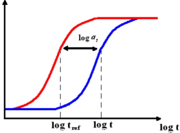
The Time-Temperature Superposition Principle, states that viscoelastic data obtained at different temperatures can be superimposed onto a master curve, using horizontal shifting along the logarithmic time, or frequency, axis and only small vertical shifts (Klompen, 1999). For these simple materials the change in temperature will shift the viscoelastic response without change in the shape of the master curve. Thus, time-temperature shift factor at(T) can

be defined as the horizontal shift to be applied to a response curve measured at an arbitrary temperature T in order to move it to the curve at some reference temperature Tref (Roylance,

2001). This shift is shown schematically in Figure 1.

The shift factor can be determined in three different ways: Arrhenius equation, Williams-Landel-Ferry Equation (WLF) or through experimental results. The Arrhenius equation is the most used method for determining the shift factor of asphalt mixtures, being represented by the equation: ⎟ ⎟ ⎠ ⎞ ⎜ ⎜ ⎝ ⎛ − = ⎟ ⎟ ⎠ ⎞ ⎜ ⎜ ⎝ ⎛ − = ref a ref t T T R E T T C

a . 1 1

. 303 , 2 1 1 . log (1)

where C is a material constant (K), Ea is the activation energy (J/mol), R is the ideal gas

constant (8.314 J/mol.K), T is the experimental temperature (K), Tref is the reference

temperature and the value 2.303 is the natural logarithm of the number 10.

In the literature different values for the activation energy for different asphalt binders can be found. These values can vary from 44 kJ / mol to 205 kJ / mol, which means that the values of C also vary for each type of asphalt mix. Medani et al. (2003) reported different values for this variable C: 10920 K, 13060 K and 7680 K.

The WLF equation is other formulation quite different that is used to calculate the shift factor of viscoelastic materials. It must be used for temperatures near or above the glassy temperature (Tg) of the material. In this formulation the displacement factor is given by:

) ( ) ( log 2 1 ref ref t T T C T T C a − + − − = (2)

where C1 and C2 are constants that depend on the material properties and reference

temperature. According to David et al. (2001), for many materials, when Tref is equal to Tg,

universal values for C1 and C2 can be used (Roylance, 2001):

) ( 6 . 51 ) ( 4 , 17 log g g t T T T T a − + − − = (3)

Alternatively, the shift factor can be determined directly from the experimental data. The measured data for the stiffness are plotted versus the logarithm of the frequency or loading time. After choosing a reference temperature the data of other temperatures are shifted horizontally to fit the curve of the reference temperature. Shifts can be obtained by extrapolation or interpolation of the original data.

3. VISCOELASTIC ANALYSIS

The analysis of viscoelastic thermorheologically simple solids, requires the solution of a convolution (or hereditary) integral that relates the current stress with a rate of strain, relaxation modulus of the material and elapsed time:

( )

_∫

∂ ∂ −

= t E d

t 0 ' ) ( τ τ ε ξ ξ σ (4)

( )

T a

t t =

ξ ₍₅₎

where a_t

( )

T is the time-temperature shift factor which has been mentioned on the previous topic. It is important to note the thermal strains (αΔT) due to the temperature variation (ΔT) were not included in Eq. (4) since the thermal expansion coefficient (α) of asphalt mixtures is not known and its determination requires costly laboratory tests.

In this work the relaxation modulus is written as a Prony-Dirichlet series:

p _{t i}

i ie E E

t

E /ρ

1 ) ( − = ∞+

∑

= (6)

where E_∞, E_iand ρ_i are the coefficients and pis the number of terms used in the series. The use of the Prony-Dirichlet series is physically motivated by the analytical solution of the differential equations of the Maxwell and Kelvin viscoelastic models.

The main idea of the stress integration algorithm is to divide time interval in a series of small steps, then the stress is computed in a successive way to each step, advancing on time (time-marching algorithm). In this algorithm, the reduced time corresponding to the next step (n+1) is obtained from the current step

( )

ξ_n through the expression:

ξ ₊ =ξ +Δξ n

n 1 (7)

where Δξ is a small reduced time increment between the two steps. Since the stresses are known in the instant ξ_n we are looking for the increment of stress (Δσ) that occurs during the increment Δξ . Then:

σ_n+1 =σ_n +Δσ ₍₈₎

Now, using Eq. (4) and applying Eq. (8) we can write:

∫

∫

− − ∂_∂ ∂ ∂ − = − =

Δ ₊ n+ ₊ n

t n t n n n dt t E dt t E 0 0 1

1 ( ) ( )

1 ε ξ ξ ε ξ ξ σ σ σ (9)

In order to simplify the above expression it is interesting to divide the first integral in two time intervals:

∫

∫

∫

− − ∂_∂ ∂ ∂ − + ∂ ∂ − =

Δ ₊ n+ ₊ n

n n t n t t n t n dt t E dt t E dt t E 0 1 0

1 ) ( ) ( )

( 1 ε ξ ξ ε ξ ξ ε ξ ξ σ (10)

Considering that the strain has a linear variation during the interval, the strain rate can be approximated as: t t Δ Δ ≅ ∂ ∂ε ε

Using this approximation and joining the integrals with the same limits, Eq (10) simplifies to

∫

∫

+ − Δ Δ + ∂ ∂ Δ =

Δ 1 ( ₊₁ )

0 n n n t t n t dt E t dt t

E ε ε ξ ξ

σ (12)

where

ΔE=

[

E(ξ_n+1−ξ)−E(ξ_n −ξ)

]

(13)

With the representation of the relaxation modulus by Eq (6), the second integral of Eq. (12) can be solved analytically:

_{( )}

⎥ ⎥ ⎦ ⎤ ⎢ ⎢ ⎣ ⎡ ⎟ ⎟ ⎠ ⎞ ⎜ ⎜ ⎝ ⎛ − Δ + Δ = ⎟ ⎟ ⎠ ⎞ ⎜ ⎜ ⎝ ⎛ + Δ Δ

∑

∫

∑

= Δ ∞ = − − ∞

+ + _p

i i i t t t p i i i n n i n n e E t T a E dt e E E

t _{1 1}

) ( 1 1 1 ρ ξ ρ ξ ξ ρ ε ε (14)

Therefore, the stress increment can be written as

Δσ =EΔε+Δσˆ (15)

where

( )

∑

= Δ ∞ _⎟⎟ ⎠ ⎞ ⎜ ⎜ ⎝ ⎛ − Δ + = p i i i

t _{E e} i

t T a E E 1 1 ρ ξ ρ (16) and

∫

Δ ∂_∂ = Δ n t dt t E 0 ˆ ε σ (17)

The two parts of Eq. (15) have different meanings. Physically, the term EΔε represents only the elastic part of the stress increment for a specific temperature, while the second term represents the viscous part of this increment also for a given temperature. Thus, the parameter E represents the instantaneous (or tangent) Young’s modulus of the material. It is important to note that this parameter depends not only on the relaxation modulus of the material, but also on the time step used in the numerical integration and the time-temperature shift factor.

Mathematically, the first term represents the stress increment due to the strain increment )

(Δε between t_n and t_n+1, while the second term (Δσˆ) represents the stress increment due to the elapsed time from the beginning of the loading process until the current time. It is important to note that each term has a dependence on time-temperature shift factor, accounting for the temperature influence on the behavior of asphalt pavements.

Using Eq. (13) we can write Eq. (17) as:

( ) dt t e e E dt t

E i i

n n

n t p

i i t ∂ ∂ ⎟ ⎟ ⎠ ⎞ ⎜ ⎜ ⎝ ⎛ − = ∂ ∂ Δ = Δ Δ − − =

∫∑

∫

ε ε

The expression above can be simplified taking out the constant terms from the integral. Thus: ( ) n i p i p i t

i dt e S

t e E e i n i n

i ˆ _{(1 )}

1 ˆ

1

1 ₀

∑

∑

∫

₌ Δ − = − Δ − − − = Δ ⇒ ∂ ∂ ⎟ ⎟ ⎠ ⎞ ⎜ ⎜ ⎝ ⎛ − − = Δ ρ ξ ρ ξ ξ ρ ξ σ ε σ (19)

Where S_incan be written as:

[ ] [ ] dt t e E dt t e E S n n i n n i n t t i t i n i _∂ ∂ + ∂ ∂ =

_∫

_∫

−

− − ε − ε

ρ ξ ξ ρ ξ ξ 1 1 0 (20)

The auxiliary variable S_in contains the hereditary part of the integral.

Now, it is necessary to observe that in the second part of Eq (20) the time interval is small, then it is possible to use again Eq (11) to do the second approximation of this algorithm. Finally, the parameter S_in is computed through the recursive expression:

( )

1

1 1 − • Δ − − Δ − ⎟ ⎟ ⎠ ⎞ ⎜ ⎜ ⎝ ⎛ − +

= n _{i i t} n

i n

i

i n

i S E a T e

e

S ρ ρ ε

ξ ρ

ξ

(21)

It can be noted from Eq (21) that the temperature effect is considered on both reduced time increment and time-temperature shift factor. Those parameters will be considered constants because constant temperature has also been considered constant. One important feature of the present formulation is that, according to Eqs. (8), (15), (16), (19) and (21), the computation of the stress at a specific step considering a constant temperature depends only on variables known at the previous step. Hence, the algorithm is very efficient in both memory and computer processing.

As it is well known, flexible pavements are multilayered systems subjected to complex loading. So, it is necessary to consider a multidimensional stress state. For a thermorheologically simple material the stresses can be calculated by:

∫

− _∂∂

= t d

t 0 ' ) ( ) ( τ τ ξ ξ ε C σ (22)

where C matrix depends on both the material property and the analysis model. The aggregates of bituminous mixtures used in asphalt pavements are randomly distributed in the space and have no preferential direction. Therefore, these mixtures can be modeled as homogenous and isotropic, provided that the material properties are determined using appropriate representative volume elements already incorporated in the test standards of these materials.

Considering that the bituminous mixtures are isotropic, their constitutive matrix (C) of can be written as:

C(t)= E(t)A(v) (23)

(Bathe, 1996). It is also worth noting that the experimental determination of the variation of the Poisson’s ratio of bituminous mixtures with time and temperature is difficult to be carried out in laboratory. As a matter of fact it is very rare to find these data published in the literature. Therefore, in the analysis of pavements the Poisson’s ratio is normally considered as constant. As a consequence, the representation of the viscoelastic behavior of these mixtures is performed by the relaxation modulus.

Considering a constant Poisson’s ratio and using Eq. (6) and Eq. (23), Eq. (22) can be rewritten as:

∫

− _∂∂

= v t E d

t

0

'

) ( ) ( )

( τ

τ ξ

ξ ε

A

σ (24)

Using Eq. (15) and Eq. (23), the stress increments for multidimensional stress states can be written as

Δσ=CΔε+Δσˆ ⇒ C = EA₍v₎ (25)

Finally, after some manipulation it can be shown that the internal variables (S) representing the stress history can be written as

( )

1

1

) ( ) 1

( −

Δ − −

Δ −

− +

= n

t i i n i n

i e E a T e v

i

i _{S A} ε

S ρ &

ξ ρ

ξ

ρ (26)

It can be noted that the recursive expression still exist and that the current step depends only on the data computed in the previous step. However, for multidimensional stress states, the internal variables are not only a number, as in the one-dimensional case, but a vector, increasing the complexity of implementation and the computational cost.

4. FINITE ELEMENT MODELING

The basic idea of the FEM is to divide a complex domain into small sub-domains with simple geometry, generally triangles and quadrilaterals in 2D and tetrahedra and hexahedra (bricks) in 3D (Bathe, 1996; Cook et al, 2002; Zienkiewicz and Taylor, 2005).

The displacement inside each finite element is interpolated using the nodal displacements (u). In general, polynomial functions are used to interpolate displacements. On the other hand, the strain vector is computed from the nodal displacements using suitable cinematic relations that depend on the problem. In a matrix form, these relations can be written as:

ε=Bu, (27)

where B is the strain-displacement matrix. This matrix is independent of the nodal displacements in geometrically linear problems (small displacement and strain).

Using the Virtual Work Principle and considering only small strains, the internal force vector (g) of a given finite element can be written as:

dV

σ

dV W

V t V

t t

∫

∫

⇒ =

=

=δug δεσ g B

The solid is in equilibrium when the internal forces are equal to the external forces (f). Therefore, at the (n+1) step:

dV

V n

t n

n

n+1 =f +1 ⇒ g +1 =

∫

B σ +1

g (29)

where, according to Eq. (25), the new stress are given by

1

1 ˆ +

+ = n + Δ = n + Δ +Δ n

n σ σ σ C ε σ

σ (30)

On the other hand, the new displacements can be computed from:

u_n+1=u_n +Δu, (31)

where Δu is the displacement increment. Using Eq. (31) and considering that Δε=BΔu we can rewrite the equilibrium equation as:

(

)

1 1

1 ˆ + +

+ =

∫

_V n + Δ = n

t

n B σ CB udV f

g ₍₃₂₎

Finally, the equilibrium equation can be written as:

KΔu=f_n+1 −gˆ_n+1, (33)

where K is the effective stiffness matrix given by

₌

∫

V

t

dV

B C B

K , ₍₃₄₎

and gˆ_n+1 is an auxiliary vector written as:

∫

∫

+ +

+ = = _V n +Δ n

t V n

t

n ˆ dV ( ˆ )dV

ˆ ₁ B σ ₁ B σ σ ₁

g ₍₃₅₎

Equations (31), (33), (34), and Eq (35) form the basis of the global algorithm for the quasistatic analysis of viscoelastic solids by FEM. As the linear viscoelastic model was adopted here, the algorithm is purely incremental and no iterations are necessary. Another important feature of this algorithm is that the stiffness matrix is constant as long as the reduced time increment (Δξ) is constant too. Finally, the stresses can be computed in any instant from recursive expression. This formulation was implemented in CAP3D program (Holanda et al., 2006) which is a finite element program for 2D and 3D analysis of flexible pavements.

5. NUMERICAL EXAMPLE

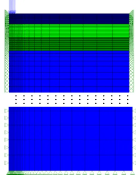
sub-base and subgrade layers are modeled as linear elastic. The thicknesses of the layers were taken as 15cm to top layer, 20 cm to base and sub-base. The subgrade, sub-base and base modulus, and the Poisson’s ratios considered are, respectively: 100MPa and 0.4; 200MPa and 0.4; 500MPa and 0.4.

A 550 kPa distributed load is applied over a circular area with a 15 cm radius (r). This load varies as a semi-sinusoidal pulse with a 0.013s of duration, which corresponds to a vehicle speed of 60 km/h. The FEM mesh is chosen so as to simulate a semi-infinite domain. The lateral limit is at a distance of 3.0 m (20r) from the symmetry axis and the bottom of the subgrade is 7.50 m (50r) bellow the surface in order to simulate an infinitely distant boundary. A finite element mesh was made with quadratic (8-node) elements with 2x2 Gauss points.

M M M M M M M M M M M M M M M

Figure 2 – Geometry and boundary conditions.

A typical Brazilian asphalt mixture was made at Universidade Federal do Ceará (UFC) using the PG 70-22 asphalt binder with a content of 5.7%, and mixed with a granite aggregate usually used in the state of Ceará. The Prony-Dirichlet coefficients for the relaxation modulus of this mix are presented in Table 1.

Table 1 – Prony Series (Tref= 25 oC) of the asphalt mixture.

Term E(Pa) ρ (s)

∞ 8.45E+08

-1 -1.53E+09 2.00E-05

2 5.04E+09 2.00E-04

3 4.86E+09 2.00E-03

4 4.28E+09 2.00E-02

5 2.89E+09 2.00E-01

6 1.78E+09 2.00E+00

7 6.13E+06 2.00E+01

8 -6.80E+04 2.00E+02

PG 70-22

It can be noted from Table 1 that the reference temperature in the Prony Series is 25ºC. The time-temperature shift factor is calculated by Arrenhius’s expression Eq. (1). In that equation a value of 10500K was attributed for C constant. This value was taken because it presented the best result to construct the master curve.

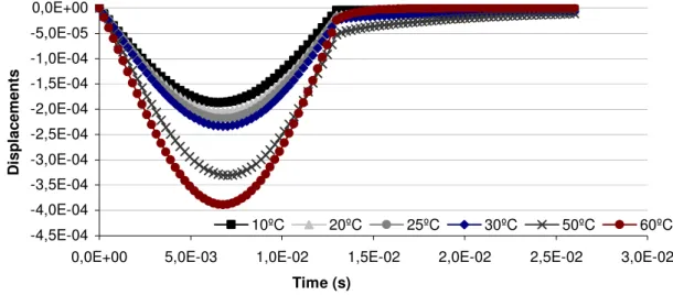
One important feature of these results is that they clearly show the significant influence of the temperature on the mechanical behavior of materials represented by viscoelastic models.

According to Figure 3 the maximum vertical displacements on the top of surface layer for different temperatures increase when the temperature increases. This fact was expected to happen because when the temperature increases the material becomes softer and more susceptible to deformation. Between the temperature of 10ºC and 60ºC it can be observed an almost 100% displacement increase, which is very significant.

-4,5E-04 -4,0E-04 -3,5E-04 -3,0E-04 -2,5E-04 -2,0E-04 -1,5E-04 -1,0E-04 -5,0E-05 0,0E+00

0,0E+00 5,0E-03 1,0E-02 1,5E-02 2,0E-02 2,5E-02 3,0E-02

Time (s)

D

ispl

acem

ent

s

10ºC 20ºC 25ºC 30ºC 50ºC 60ºC

Figure 3 – Displacement on the top of surface layer.

Figure 4 shows the horizontal stresses on the base of the surface layer for the same temperature range. It is observed that when the temperature increases the horizontal stress initially increases too. However, for higher temperature the stress starts to be reduced and finally for even higher temperatures like 50ºC and 60ºC the stress values change from tension to compression.

-4,0E+04 -3,5E+04 -3,0E+04 -2,5E+04 -2,0E+04 -1,5E+04 -1,0E+04 -5,0E+03 0,0E+00 5,0E+03

0,00E+00 5,00E-03 1,00E-02 1,50E-02 2,00E-02 2,50E-02 3,00E-02

Time (s)

S

tress X

X

10ºC 20ºC 25ºC 30ºC 50ºC 60ºC

Figure 4 – Horizontal stress (σxx) on the base of surface layer.

tension to compression indicated that for these high temperatures the surface layer is totally compressed and can not carry-out adequately its main structural function which is to distribute the wheel loads in a large area resisting the resulting stress mainly by bending. As a consequence high compressive vertical stress will be generated in the sub-layers which can lead to the permanent deformation (rutting) of the pavement.

6. CONCLUSIONS

The present work presented a simple incremental algorithm to thermo-viscoelastic analysis of viscoelastic solids using the Finite Element Method. This algorithm is based on time discretization of the convolution integral (hereditary integral) and the representation of the relaxation modulus as a Prony-Dirichlet series. The thermal effects are included in the analysis using the Time-Temperature Superposition Principle, since laboratory tests show that bituminous mixtures present a thermorheologically simple behavior.

In order to adequately represent multidimensional stress states of isotropic materials the effects of the relaxation modulus and Poisson’s ratio are treated separately in the constitutive matrix, with the latter is considered as a constant. The adopted approach allows both simplifying the implementation and using directly the properties obtained from creep tests performed in asphalt mixes. This is important for practical applications since most finite element programs use the hydrostatic-deviator split which is not convenient for bituminous mixtures since the Prony Dirichlet series for bulk and shear modulus are not easily obtained from laboratory tests.

The present time-marching algorithm is rather efficient from the computational point of view, since the computation of displacements and stresses in each step uses only the values of the previous step. In addition the stiffness matrix remains constant for a constant time increment and needs to be assembled and factorized only once.

Finally, the results obtained in the stress analysis of a pavement considering different temperatures for the asphalt layer demonstrated the importance of the consideration of this parameter in pavement design. Higher temperatures lead to higher displacements and greatly affect the horizontal stresses, which can even change from tension from compression.

Acknowledgements

The authors gratefully acknowledge the financial support provided by FUNCAP, CNPq, ANP and FINEP agencies to the development of this work.

REFERENCES

Bathe, K.J. (1996) Finite Element Procedures. New Jersey, Prentice Hall.

Chabot A., Tamagny P., Poché D. , Duhamel D. (2006). Visco-elastic modelling for asphalt pavements – software ViscoRoute. 10th International Conference on Asphalt Pavements. Québec.

Cheung, C.Y. (1995). Mechanical Behavior of Bitumens and Bituminous Mixtures. Ph. D Dissertation. University of Cambridge, Cambridge, UK.

Dubois, F., Arfaoui, M. Laveissiere, D., Petit, C. (1999). A Finite Element Thermoviscoelastic Model: Application to Pavement Structures. 13th Engineering Mechanics Conference, ASCE, Baltimore.

Elseifi, M.A., Al-Qadi, I.L., Yoo, P.J., (2006). Viscoelastic Modeling and Field Validation of Flexible Pavements. Journal of Engineering Mechanics, Vol. 132, No 2, p. 172-178.

Holanda, A. S., Parente Jr., E., Araújo, T. D. P., Melo, L. T. B., Evangelista Jr., F., Soares, J. B., (2006). An Object-Oriented System for Finite Element Analysis of Pavements. Proceedings of the III European Conference on Computational Mechanics (ECCM), p. 1-17, Lisboa.

Huang, Y. H, (2004). Pavement Analysis and Design. 2.ed. Pearson Prentice Hall, Upper Saddle River, NJ, USA.

Klompen, E.T.J., Govaert, L.E., (1999). Nonlinear Viscoelastic Behaviour of Thermorhologically Complex Materials. Mechanics of Time-Dependent Materials, Vol. 3, No 1, p. 49-69.

Lakes, R. S. (1998). Viscoelastic Solids. CRC Press.

Lu, Y., Wrigth, P., (2000). Temperature Related Visco-Elastoplastic Properties of Asphalt Mixtures. Journal of Transportation Engineering, Vol. 16, No 1, p. 58-65.

Medani, T. O., Huurman, M. (2003). Constructing the Stiffness Master Curves for Asphaltic Mixes. ISSN 0169-9288.

Muliana, A., Khan, K. A. (2008). A time-integration algorithm for thermo-rheologically complex polymers. Computational Materials Science. Vol. 41, pp. 576-588.

Roylance, D. (2001). Engineering Viscoelasticity. Massachusetts Institute of Technology, Cambridge, MA.

Sawant, S. Muliana, A. (2008). A thermo-mechanical viscoelastic analysis of orthotropic materials. Composite Structures. Vol. 83, pp. 61-72.

Shames, I. H; Cozzarelli, F. A. (1997) Elastic and Inelastic Stress Analysis. Taylor & Francis, Revised Printing.

Shen, Y. P.; Hasebe, N.; Lee, L. X. (1995) The finite element method of three-dimensional nonlinear viscoelastic large deformation problems. Computers & Structures, v. 55, n. 4, pp. 659-666.

Taylor, R.L., Pister, K.S., Goudreau, G.L. (1970). Thermomechanical Analysis of Viscoelastic Solids. International Journal for Numerical Methods in Engineering, Vol. 2, No. 1, p. 45-59.

Wong. W., Zhong, Y. (2000). A Three-Dimensional Finite Element Formulation for Thermoviscoelastic Orthotropic Media. Journal of Transportation Engineering (ASCE), Vol. 126, (1) p. 46-49.

Zienkiewicz, O.C, Taylor, R.L.E. (2005). The Finite Element Method for Solid and Structural Mechanics. Massachusetts. Elsevier.