MIMO channel modeling and estimation: application of spherical harmonics and tensor

(1)

FEDERAL UNIVERSITY OF CEARÁ

DEPAR TMENT OF TELEINFORMATICS ENGINEERING POSTGRADUATE PROGRAM INTELEINFORMATICS ENGINEERING

MIMO Channel Modeling and Estimation:

Application of Spherical Harmonics and Tensor

Decompositions

Master of Science Thesis

Author

Leandro Ronchini Ximenes

Advisor

Prof. Dr. André Lima Ferrer de Almeida

(2)

LEANDRO RONCHINI XIMENES

MIMO CHANNEL MODELING AND ESTIMATION:

APPLICATION OF SPHERICAL HARMONICS AND

TENSOR DECOMPOSITIONS

Dissertação apresentada à Coordenação do Programa de Pós-graduação em Engenharia de Teleinformática da Universidade Federal do Ceará como parte dos requisitos para obtenção do grau deMestre em Engenharia

de Teleinformática.

Área de concentração: Sinais e Sistemas

Orientador: Prof. Dr. André Lima Ferrer de Almeida

(3)

Dados Internacionais de Catalogação na Publicação Universidade Federal do Ceará

Biblioteca de Pós-Graduação em Engenharia - BPGE

X34m Ximenes, Leandro Ronchini.

MIMO channel modeling and estimation: application of spherical harmonics and tensor decompositions / Leandro Ronchini Ximenes. – 2011.

120 f. : il. color. , enc. ; 30 cm.

Dissertação (mestrado) – Universidade Federal do Ceará, Centro de Tecnologia, Departamento de Engenharia de Teleinformática, Programa de Pós-Graduação em Engenharia de Teleinformática, Fortaleza, 2011.

Área de concentração: Sinais e Sistemas.

Orientação: Prof. Dr. André Lima Férrer de Almeida.

1. Teleinformática. 2. Decomposições tensoriais. 3. Antenas - Otimização. I. Título.

(4)

Abstract

I

n the last two decades, multiple input multiple output (MIMO) wireless systems have beensubject of intense research due to the theoretical promise of the proportional increase of the communications channel capacity as the number of antennas increases. This outstanding property supposes an efficient use of spatial diversity at both the transmitter and receiver. An important and not well explored path towards improving MIMO system performance using spatial diversity takes into account the interactions among the antennas and the (physical) propagation medium. By understanding these interactions, the transmit and receive antenna arrays can be designed to best “match” the propagation medium so that the link quality and capacity can be further improved in a MIMO system. In this work, we consider the use of spherical harmonics and tensor decompositions in the problem of MIMO channel modeling and estimation. The use of spherical harmonics allows to represent the radiation patterns of antennas in terms of coefficients of an expansion, thus decoupling the transmit and receive antenna array responses from the physical propagation medium. By translating simple propagation-motivated channel models with polarization information into the spherical harmonics domain, we study how propagation parameters themselves and antenna configurations affect MIMO performance in terms of capacity and correlation. A second part of this work addresses the problem of estimating directional MIMO channels in the spherical harmonics domain using tensor decompositions. Considering both single-scattering and double-scattering propagation scenarios, we make use of the parallel factor (PARAFAC) and PARATUCK-2 decompositions, respectively, to estimate the propagating spherical modes, from which the directions of arrival (DoA) and directions of departure (DoD) can be extracted. Finally, we propose and compare two methods for optimizing the coefficients of the spherical harmonics expansion of an antenna array for a prespecified MIMO channel response.

Keywords: MIMO channel modeling, spherical harmonics, tensor decompositions,

(5)

Resumo

Nas últimas décadas, sistemas de comunicação sem fio de múltiplas antenas (MIMO -Multiple Input -Multiple Output) têm sido objetos de intensas pesquisas devido à promessa teórica do aumento proporcional da capacidade com o aumento do número de antenas. Esta propriedade excepcional supõe um uso eficiente da diversidade espacial no transmissor e receptor. Um caminho importante e não bem explorado no sentido de melhorar o desempenho de sistemas MIMO usando diversidade espacial leva em conta a interação entre as antenas e meio de propagação (físico). Através da compreensão dessas interações, arranjos de antenas de recepção e transmissão podem ser projetados para melhor "casar" com o meio de propagação, tal que a qualidade dolink de comunicação e capacidade possam ser melhoradas em um sistema MIMO. Neste trabalho, consideramos o uso de harmônicos esféricos e decomposições tensoriais no problema de modelagem de canal MIMO e estimação. O uso de harmônicos esféricos permite representar os padrões de radiação de antenas em termos de coeficientes de uma expansão, assim desacoplando as respostas dos arranjos de antenas (transmissoras e receptoras) do meio de propagação física. Traduzindo modelos simples de canais baseados em propagação, com informações de polarização, para o domínio dos harmônicos esféricos, estudamos como os parâmetros de propagação si e configurações específicas de antenas afetam o desempenho do sistema MIMO em termos de capacidade e de correlação. A segunda parte deste trabalho aborda o problema de estimar canais direcionais MIMO no domínio dos harmônicos esféricos usando decomposições por tensores. Considerando tanto cenos de espalhamento simples e de duplo espalhamento, fazemos uso das decomposições PARAFAC e PARATUCK2, respectivamente, para estimar os modos esféricos propagantes, a partir das quais as direções de chegada (DoA) e as direções de saída (DoD) podem ser extraídas. Finalmente, propomos e comparamos dois métodos de otimização dos coeficientes da expansão em harmônicos esféricos de arranjos de antenas para respostas de canais MIMO pré-especificados .

Palavras-chave: MIMO, harmônicos esféricos, decomposições tensoriais, PARAFAC,

(6)

Dedicatories

“A verdade é que a gente não faz filhos. Só faz o layout. Eles mesmos fazem a arte-final.”

- Luís Fernando Veríssimo

(7)

Acknowledgements

Although this work was somewhat limited within a period of two years, with well-defined beginning and end, it is not a sudden rupture on what I have done these past few years. Maybe a very special step in my life, a desired rite of passage. Anyway, there was a before, and there will be an after. Thus, I would like here to give thanks that are not delimited exclusively by the time of completion of this thesis.

Starting by justice and symbolism of this work, firstly I would like to thank those who were present this side of my professional life. First the most sincere thanks to my advisor, prof. André Lima Ferrer de Almeida. Whether by the relative small difference of our ages or mostly because of his natural enthusiasm for researching, he seemed very attentive to my questions of technical, professional and personnel matters. Moreover, I would like to thank all members of the GTEL whom I lived good moments in these special years.

Not restricting thanks to my colleagues, I will be brief to thank my family and my friends around the world, especially those living in Fortaleza. Thank you all for supporting me, making sacrifices, and understading my own ones. I am fully aware that my work is a part of my happyness, which I wish I could share with all of you.

(8)

List of Symbols

θ Elevation angle

φ Azimuth angle

ρpc Complex pattern correlation

ρsc Sub-channel correlation

Nmp Number of multipaths

F Number of symbols in a data block

P Number of transmit antennas

Q Number of receive antennas

K Number of time-slots

Lr Spherical harmonics order for receive array

Lt Spherical harmonics order for transmit array

Mr Number of spherical modes for receive array

Mt Number of spherical modes for transmit array

R1 Number of scattering clusters seen by receive array

R2 Number of scattering clusters seen by transmit array

DoA Direction of Arrival

DoD Direction of Departure

XP R Cross-polarization ratio

a Receive antenna spherical harmonics coefficients vector b Transmit antenna spherical harmonics coefficients vector yr Receiving spherical harmonics base

yt Transmitting spherical harmonics base

A Receive array response matrix B Transmit array response matrix

Yr Receiving clusters’ spherical harmonics matrix

Yt Transmitting clusters’ spherical harmonics matrix

G Inter-cluster gain matrix M Mode-to-mode matrix H Channel matrix

Cr Receiving clusters’ gain matrix

Ct Transmitting clusters’ gain matrix

(9)

Notation

In this thesis the following conventions are used. Scalar variables are denoted by upper-case letters (A, B, . . .), vectors are written as boldface lower-case letters (a,c, . . .), matrices correspond to boldface capitals (A,B, . . .), and tensors are written as calligraphic letters(A,B, . . .). The meaning of the following symbols are, if nothing else is explicitly stated:

C set of complex-valued numbers

CI set of complex-valued_I-dimensional vectors

CI×J _{set of complex-valued (}_I_×_J_)-matrices

CI1×···×IN set of complex-valued (_I1_{× · · · ×}_I

N)-tensorsa∗

complex conjugate ofa∈C_|a_| modulus ofa

ka_k1 l-1 norm ofa kak

l-2 norm ofa 1exAT transpose ofA

AH Hermitian transpose ofA

A−1 _{inverse of}_A

A† _{Moore-Penrose pseudo-inverse of}_A

kA_kF(kAkF) Frobenius norm ofA(A)

IN Identity matrix of dimensionN.

[A]i1,i2 =Ai1,i2 (i1, i2)-th element of matrixAI1×I2.

[A]i1·([A]·i2) i1-th row (i2-th column) ofA.

[A]i1,i2,i3 =Ai1,i2,i3 (i1, i2, i3)-th element of tensor A.

A_⊗B The Kronecker product ofAI×J withBK×L,

A_⊗B=

    

A1,1B A1,2B · · · A1,JB

A2,1B A2,2B · · · A2,JB

..

. ... ...

AI,1B AI,2B · · · AI,JB

    

IK×JL

.

A_⋄B The Khatri-Rao (column-wise Kronecker) product. ForAI×K andBJ×K,

A_⋄B= [A·1⊗B·1, . . . , A·K⊗B·K]IJ×K.

vec(A) The vectorization operator.

ForAI×J: vec(A)=

  

A·1

.. . A·J

  .

(10)

List of Figures

2.1 Spherical Harmonics . . . 24

2.2 Spherical harmonics coefficientsversus translation. A dipole example . . . 26

2.3 Communications’ tensors. Receive signal and channel . . . 27

2.4 Tucker model . . . 28

2.5 PARAFAC model . . . 29

2.6 PARATUCK2 model . . . 29

3.1 Imaginary sphere surrounding an antenna. . . 31

3.2 MIMO system withP receive antennas andQtransmit antennas . . . 33

3.3 Absolute values of matrix M. Y-axis has the modes at the receiving side (DoA), and X-axis has the modes at the transmiting side (DoD) . . . 41

3.4 Absolute values of matrix M. Y-axis has the modes at the receiving side, and X-axis has the modes at the transmiting side . . . 42

3.5 Y−1 1 pattern (dipole) . . . 43

3.6 Ergodic capacityvssingle cluster angle. Antennas are dipoles . . . 43

3.7 Y0 1 pattern. . . 44

3.8 Mode-to-mode matrixMfor different cluster’s position . . . 44

3.9 capacityvs cluster’s DoD, for antennas of different correlations . . . 45

3.10 CapacityversusSNR (dB) for different number of cluster. 2×2MIMO analysis for randomly positioned clusters. . . 46

3.11 CapacityversusSNR (dB) for different number of cluster. 4×4MIMO analysis for randomly positioned clusters. Capacity versusSNR (dB) . . . 46

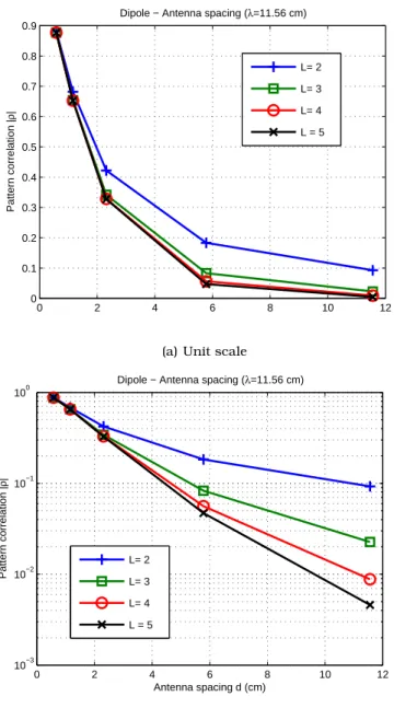
3.12 CapacityversusSNR (dB) for different antenna spacing. λ= 11.80cm (f = 2.56GHz)47 3.13 Pattern Correlation for different antenna spacing and different truncated order L.λ= 11.56cm (f = 2.56GHz). . . 48

3.14 Physical mockups (prototypes) whose antenna placements served to create the simulated mockups. Mockup/prototype 1 and Mockup/prototype 2 are also designed as low and high correlation mockups, respectively . . . 49

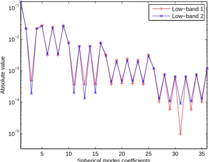
3.15 Antennas’ positioning in the two mockups. Mockup 1 (left) and Mockup 2(right) 49 3.16 Radiation patterns (absolute/radial, vertical and horizontal) for the two antennas (LB1 and LB2) of the mockups. They are designed low band antennas to work at 700 MHz. Patterns reconstructed using spherical harmonics coefficients extracted from CST patterns . . . 50 3.17 Absolute values of spherical harmonics coefficients for antennas LB1 and LB2 . 50

(14)

LIST OF FIGURES 13

3.18 Pattern correlation between antenna LB1 and LB2 for the two mockups versus

truncated number of spherical orders. . . 51

3.19 CapacityversusSNR. (a) Lossless antennas; (b) Mockups with efficiency losses . 51 3.20 Ergodic capacity mean for WINNER II CDL models.. . . 53

3.21 Ergodic capacity variance for WINNER II CDL models. . . 54

4.1 MIMO channel tensor . . . 57

4.2 Single-scattering mode-to-mode channel tensor. . . 59

4.3 Single-Scattering Cluster DoD estimation using correlation approach . . . 63

4.4 ALS-PARAFAC: MdSEversus iterations. . . 67

4.5 Single-scattering directions estimation . . . 69

4.6 Double-scattering mode-to-mode tensor . . . 71

4.7 Double-scattering example . . . 72

4.8 ALS-PARATUCK-2: MdSEversusiterations . . . 77

4.9 ALS-PARATUCK-2 for (R1= 2, R2= 3): MdSEversus SNR . . . 78

4.10 ALS-PARATUCK-2 for (R1= 3, R2= 3): MdSEversus SNR . . . 78

4.11 Double scattering multipath (dashed line) in a single-scattering model . . . 79

4.12 PARAFAC error modelling PARATUCK-2. MdSEversusSNR. . . 80

5.1 Steepest-Descent antennas optimization. Ergodic capacity vs Spherical orderL . 86 5.2 Steepest-Descent pattern optimization . . . 87

5.3 Absolute pattern correlation on each optimized array. . . 87

5.4 Steepest-Descent antennas optimization. Ergodic capacity vs Number of antennasN . . . 88

5.5 Computational cost comparison between GN and SD with different adaptation steps . . . 89

5.6 SD optimization for bidirectional channels with progressive addition of single-scattering clusters.5.6(b)-5.6(e) illustrate some optimized radiation patterns90 5.7 Multiplexing scheme over spherical harmonics . . . 93

A.1 GUI simulator . . . 96

A.2 Antennas panel. . . 97

A.3 Import external antenna . . . 98

A.4 Channel panel . . . 99

A.5 Metrics panel . . . 100

A.6 Layers diagram of the simulator . . . 101

A.7 Uniformly spaced clusters channel . . . 102

A.8 Randomly spaced clusters channel . . . 103

A.9 "One-ring" channel. . . 104

A.10“Upload channel” pop-up window . . . 104

A.11WINNER II CDL table . . . 105

B.1 Ergodic Capacity (bps/Hz) for SIMO and MIMO cases at A1 NLOS scenario. . . . 107

B.2 Correlationρ12and Ergodic Capacities (bps/Hz) for scenario A1 NLOS. . . 108

B.3 Ergodic Capacity (bps/Hz) for SIMO and MIMO cases at B1 NLOS scenario. . . . 109

B.4 Correlationρ12and Ergodic Capacities (bps/Hz) for scenario B1 NLOS. . . 110

B.5 Ergodic Capacity (bps/Hz) for SIMO and MIMO cases at B2 NLOS scenario. . . . 111

(15)

LIST OF FIGURES 14

B.7 Ergodic Capacity (bps/Hz) for SIMO and MIMO cases at C1 NLOS scenario. . . . 113 B.8 Correlationρ12and Ergodic Capacities (bps/Hz) for scenario C1 NLOS. . . 114

(16)

List of Tables

2.1 Tensor decompositions . . . 27

4.1 Kruskal’s conditions for single-scattering scenarios . . . 62

5.1 GN computational cost . . . 88

5.2 SD computational cost -†Not achieved convergence . . . 88

(17)

Chapter

1 Introduction

1.1 Work context and proposal

In the last two decades, multiple input multiple output (MIMO) wireless systems have been the subject of intense research due to the theoretical promise of the proportional increase of the capacity as the number of antennas increases [1], [2]. This outstanding property occurs by the employment of so-called spatial diversity at both the transmitter and receiver, in addition to diversities in frequency and in time [3]. The spatial diversity enables a new point of view of the relations among the elements of the physical layer and the cross-layers interrelationships. There is almost a consensus that the next steps to be taken in improving the system performance using spatial diversity should take into account the interaction among the antennas and the propagation medium in a more general way [4].

Although there are several channel models in the literature which intend to separate the responses of arrays of antennas from the propagation medium ([ [5], [6]]), few are analytical ones based on the propagation of multipaths. A relatively recent proposal [7] was to use the scalar spherical harmonic expansion to completely dissociate the radiating elements (antennas) from the propagation medium. The basic idea of MIMO channel modeling using spherical harmonics as it is known today started in [5], where the MIMO channel matrix of the system could be factored into fixed (and known) and random matrices where the deterministic portion depends on receiver and transmitter antenna configurations. In this first case, the scattering did not have information on the multipath components. In addition, the model was limited only to the omnidirectional radiation patterns. Before this work, the use of spherical harmonics was mostly used in arrays of microphones and acoustic applications [8]. In [9], the spherical harmonics were used for different radiation patterns, which allowed a greater generalization of the MIMO channel model using spherical harmonics. It is worth noting that previous works on the subject are restricted to somewhat idealistic MIMO channels which are scattering-rich propagation. An important step toward the generalization of the channel model is given in [7], where it introduces the mapping structure of spherical modes that is most often used today (and in this work). This structure enables to fully describe the propagation scenario in the spherical harmonics domain. The drawback of [7] is that polarization, despite described, is presented as a function of only the propagation medium, ignoring antennas’ polarization. This problem is overcome in [6] by using the vector spherical harmonics [10]. However, it lacks of the propagation medium proper realistic detailment.

(18)

1.2. Summary of contributions 17

work, diffuse channel models were combined to take advantage of the different approaches. Each specific element of the communication system (e.g. multipath, antenna and scattering cluster) is described in a clear and concise form. As a consequence, all elements can be modeled one by one, even with respect to its polarization.

Another tool that has been applied recently to the problem of modeling and estimation of wireless propagation channels is the tensor decomposition. In a few recent works ( [11], [12], [13], [14]), the parallel factor (PARAFAC) decomposition ( [15], [16], [17], [18]) has been used to model and estimate parametric multipath channels. The work [11] proposes a training sequence based trilinear alternating least squares (ALS) estimator for single input multiple output (SIMO) channel parameters such as directions of arrival, relative propagation delays and fading amplitudes of the multipaths. This work is generalized later in [12] to MIMO channels. In [14], a quadrilinear ALS estimator is proposed to extract the channel parameters based on previous knowledge (or unstructured estimation) of the MIMO channel. A common feature of these works is the simplifying assumption of single-scattering propagation. Moreover, to the best of the author’s knowledge the combination of spherical harmonics and tensor decompositions for modeling/estimation of MIMO channels have not been addressed yet in the literature.

In this work, we consider the use of spherical harmonics and tensor decompositions in the problem of MIMO channel modeling and estimation. The use of spherical harmonics allows to represent the radiation patterns of antennas in terms of coefficients of an expansion, thus decoupling the transmit and receive antenna array responses from the physical propagation medium. By translating simple propagation-motivated channel models with polarization information into the spherical harmonics domain, we study how propagation parameters and antenna configurations affect MIMO performance in terms of capacity and correlation. A second part of this work addresses the problem of estimating directional MIMO channels in the spherical harmonics domain using tensor decompositions. Considering both single-scattering and double-scattering propagation scenarios, we make use of the parallel factor (PARAFAC) and PARATUCK-2 decompositions, respectively, to estimate the propagating spherical modes, from which the directions of arrival (DoA) and directions of departure (DoD) can be extracted. Finally, we propose and compare two methods for optimizing the coefficients of the spherical harmonics expansion of an antenna array for a prespecified MIMO channel response.

1.2 Summary of contributions

In this work we propose three main branches of contributions:

◮ Analysis of the spherical harmonics expansion in MIMO systems - As previously

mentioned, the MIMO channel model decomposed into spherical harmonics presented in this thesis has the advantage over similar models by presenting a more concise and functional form. The degree of freedom presented by this new format allows punctual or global analysis of elements of the channel on the system performance. The major contribution here is to demonstrate the impact of the order of truncation of spherical harmonics, the spacing among the antennas and the number of clusters seen in the domain of spherical harmonics. Simulations involving antennas and realistic scenarios (e.g. WINNER II CDL) illustrate the flexibility of the model.

◮ Combination of algorithm PARAFAC-ALS and ALS-PARATUCK2 with MUSIC method

or correlation-based to extraction ofDoA/DoDpair- Different methods for estimating

(19)

1.3. Organization 18

including the widespread MUSIC-like algorithms, are based on the use of the channel matrix (considering the presence of antennas) to identify the directions of arrival and departure. Also, it is not new the use of tensor decomposition (PARAFAC) to estimate these parameters, even allowing joint estimation of others, as transmitted symbols. The contribution of this thesis is to develop two methods where it is possible to estimate these parameters, inherent to the propagation medium, disregarding the influence of the antennas. It is possible by modeling the channel through the PARAFAC decomposition for single-channel scattering scenarios and with PARATUCK2 decomposition for double-scattering channels.

◮ Analysis of Gauss-Newton and Steepest-Descent optimization algorithms of

antenna arrays for channels using spherical harmonics expansion- Channel models

that have elements corresponding to the antenna arrays as explicit terms in their equations, as the Kronecker or the Finite-Scatterer models, naturally have great appeal for applications of antenna optimization. Usually such methods have a metric to optimize (e.g. increase capacity and/or minimize interference between antennas) by changing the construction parameters, such as the position of the antennas. Because of the possibility of complete separation between the arrays of antennas from the propagation medium due to the model using spherical harmonics, this thesis presents two methods of optimization of antennas that aim to optimize the capacity of MIMO system by changing the coefficients of the spherical expansions. The change of these coefficients can be translated both in change of radiation pattern itself and in translation and/or rotation of the antennas. As a result of flexibility of solutions, the optimization techniques presented here can address a wide range of design constraints, yet with low complexity.

1.3 Organization

The structure of this thesis is divided into the following chapters (with respective descriptions of their subsections):

Chapter 2 - This chapter provides a quick overview of the trinity of theoretical fundamentals

discussed in this thesis: MIMO channel modeling, spherical harmonics and tensor decomposition. The information shown here, albeit basic, will serve as a motivating starting point for the deductions shown throughout this material.

Chapter 3 - This chapter deals with MIMO channel modeling using spherical harmonics. The

channel is treated as a conventional channel matrix, but where elements belonging to the antennas and the propagation medium can be completely decoupled. Simulations show applications and conclusions that are often already known for conventional channels, but are seen here through the lens of spherical harmonics.

◮ Section 3.2- Plane Wave Representation for an Antenna - The planewave

representation and spatial product of two functions in the spherical harmonics domain are derived.

◮ Section 3.3- MIMO Channel Decomposition Using Spherical Harmonics - The

MIMO channel model is presented in different forms, including now polarization.

◮ Section 3.4- Antenna Translation and Rotation - Higher degree of freedom for

physical construction/manipulations of arrays are possible with new developments.

◮ Section3.5-Capacity and Correlation for MIMO Systems -Classical formulas for

(20)

1.4. Publications 19

◮ Section 3.6- Simulations and Discussions - Final studies about the previous

sections are displayed, involving basically several simulations. Characteristics of wave propagation, antennas’ spacing, WINNER II model analisys are simulated and discussed.

Chapter 4 - Extending the channel matrix to a tensor model, this chapter presents a quite

different approach for MIMO systems. The innovative factor shows up as the possibility to model (single and double) scattering scenarios using both spherical harmonics and tensors. Techniques to estimate directions of arrival and departure are developed as natural applications for this new approach.

◮ Section4.2-Tensorial representation of the channel model -This section shows

a generic tensor representation of the MIMO channel using spherical harmonics decomposition. The model previously presented in Chapter 3 is resumed, adding a third dimension: time.

◮ Section 4.3- Single scattering channels - The channel presented in the previous

section is particularized as a single-scattering channel. It is then treated as a PARAFAC model, leading to discussion about its caracteristics (e.g. uniqueness), and finally to estimation ofDoA/DoDthrough new techniques discussed here, such a MUSIC-like and a correlation-based methods.

◮ Section 4.4- Double scattering channels - The last major section of this chapter

expands the channel model using tensor for bidirectional channels. The more generalized channel resulted in the use of a more comprehensive tensor model-the PARATUCK-2. Estimation ofDoD/DoAare again discussed, taking into account new factors arising from this new possibility.

Chapter 5 - The channel model presented in Chapter 3 is used here for the development and

analysis of two antenna array optimization techniques. In addition, the chapter provides a brief insight into the meaning of the spherical modes for traditional channels, such as the Kronecker and the full-correlation matrix.

Chapter 6 - A general conclusion about this thesis is presented, highlighting new research

perspectives.

1.4 Publications

The list of contributions includes conference papers and technical reports.

◮ L. R. Ximenes and A. L. F. de Almeida, "Antenna array optimization for channel

model using spherical harmonics decomposition", 29th Brazilian Symposium on Communications (SBrT’11), Curitiba, Paraná, Brazil, October 2011.

◮ L. R. Ximenes and A. L. F. de Almeida, "Performance Evaluation of Mobile

Phone Antennas in Physical MIMO Channels Using Polarized Spherical Harmonic Decomposition", IEEE 74th Vehicular Technology Conference - VTC Fall 2011, San Francisco, California, USA, September 2011.

◮ L. R. Ximenes and A. L. F. de Almeida, "Capacity Evaluation of MIMO Antenna

(21)

Chapter

2 Fundamentals: Channel models,

Spherical harmonics and Tensors

2.1 Channel models

The promising MIMO theoretical capacity gain presented in ( [1], [2]) have considered an idealized perfect channel model. Typical wireless scenarios, such as indoor or macro-urban environments, have intrinsic characteristics responsible for changing communication systems in different ways. These characteristics have much to do with the physical components (e.g. buildings, walls, etc.) present in each scenario. Thus, more realistic channel models have been proposed over recent years to supply consistent information for research in the area.

There are several ways to classify the large number of channels models. Among the basic properties that one can fit into are the dualities narrowband (flat fading) vs. broadband (frequency-selective), time-varying vs. time-invariant. Another important classification divides the channel model as being analytical or physical.

This section will briefly comment on few very well-known models. It is a brief overview about the evolution of models to the state of the art, so that the channel model presented in this thesis can be introduced and compared.

This first part of this section will focus on channels based on correlation metrics, and the second one will approach propagation-based models.

2.1.1 Correlation-based models

Mathematically, MIMO channel models are represented by a P ×Q complex matrix H. Thus, the element Hpq element of this matrix represents the channel gain between the p-th

receive antenna and theq-th transmit antenna. In general, each element of this matrix can be decomposed into LOS and NLOS components.

The correlation-based models usually try to describe the channel in a stochastic way. More specifically, the channel is described in terms of the correlation among the antennas. This type of model usually uses the metric of correlation to generalize different propagation scenarios at the cost of lacking particularity to model specific details, like the directions of arrival/departure and doppler shifts.

(22)

2.1. Channel models 21

2.1.1.1 The i.i.d. model

The independent and identically distributed (i.i.d.) model represents the rich scattering channel, where all elements of the matrix H are statistically independent, and therefore uncorrelated.

Physically, the rich scattering scenario can be pictured as when the multipaths have uniform distribution of directions of arrival and departure surrounding the antenna arrays, as well as for power of scattered rays. The distintiction between the terms i.i.d. and rich scattering should be considered when there are correlated antennas. In this case, it may be said that the scenario is of rich scattering propagation, although the channel is not necessarily i.i.d.

2.1.1.2 Full-correlation matrix

A MIMO channel can be completely represented by the full-correlation matrix, whose equation is given as follows

Rhh=E{hhH}, (2.1)

whereh=vec(H).

Each element of the full-correlation matrix is a correlation coefficient between any two antennas of a MIMO system, including the autocorrelations. Thus, the matrix in (2.1) has dimensionsP Q×P Q. This large size makes the model impractical, so several other models have been proposed.

2.1.1.3 The Kronecker model

The Kronecker model is a particularization of the full-correlation matrix model. It is supposed that when the BS and MS are far apart, then the propagation medium is sufficient to decorrelate transmitting from receiving arrays. Thus, the complexity of the full correlation model is avoided.

The model equation is

H_kron=_p 1 tr{Rrx}

R1_rx/2G(R1_tx/2)T, (2.2)

where Rrx = E{HHH} and Rtx = E{(HHH)T} are the receive and transmit autocorrelation

matrices respectively, and G is the i.i.d. gaussian matrix that decorrelates both antenna arrays in a point-to-point MIMO communication. However, this often is not true. Long distances between the BS and MS usually generate the keyhole effect, but not necessarily the expected decorrelation.

More general models such as the Weichselberger channel model( [3]) were proposed to relax the restriction of the Kronecker model and to allow for any arbitrary coupling between the transmit and receive link sides.

2.1.2 Propagation-motivated analytical models

2.1.2.1 Finite-scatterer model

(23)

2.1. Channel models 22

H(f, t) = √ 1

R2R1     

ej(φ1,1+2π ur

11v_r

c t) · · · ej(φ1,r1+2π ur

1r1vr

c t)

..

. . .. ...

ej(φ1,1+2π ur

11v_r

c t) · · · ej(φp,r1+2π ur

pr1vr

c t)

         

Cr(1) 0 · · ·

0 ... 0

..

. 0 Cr(R1)

    

×[ΘR1×R2⊙DR1×R2(f)]× 

   

Ct(r2) 0 · · ·

0 . .. 0

..

. 0 Ct(R2)

         

ej(ψ1,1+2π ut

11v_t

c t) · · · ej(φ1,st+2π

ut 1stv_t

c t)

..

. . .. ...

ej(ψ1,1+2π ut

11v_t

c t) · · · ej(ψq,st+2π

ut

qstv_t

c t)

     , (2.3)

where⊙is the Hadamard product and

DR1×R2(f) =    

e−j2πf τ1,1 _{· · ·} _e−j2πf τ1_,st ..

. . .. ...

e−j2πf τr1,1 _{· · ·} _e−j2πf τr1,r1     , (2.4) and:

◮ R1 - Number of receive scattering clusters; ◮ R2 - Number of transmit scattering clusters; ◮ f - carrier frequency (Hz);

◮ t- time (s);

◮ vr- vector speed (m/s) of receive array; ◮ vt- vector speed (m/s) of transmit array;

◮ s_ij(t)- the signal between the receiving antennaj and the scattereri; ◮ φ_i,j - the angle of departure from thej-th receive antenna to theiscatterer; ◮ ψ_i,j- the angle of departure from thej-th transmit antenna to theiscatterer; ◮ C_r(r1)- average power of ther1-th scatterer seen by the receiver;

◮ C_t(r2)- average power of ther2-th scatterer seen by the transmitter; ◮ D_R₂_×_R₁(f)- Delay matrix linking each pairDoA-DoD;

◮ ΘR1×R2 - Gain matrix linking each pairDoA-DoD.

A more concise form of the channel model in (2.3)can be arranged as

H(f, t) = √ 1

R2R1Ψ[ΘR1×R2⊙DR1×R2(f)]Φ

T_, _(2.5)

(24)

2.2. Spherical harmonics 23

This channel model can be considered one of best models that best describe realistic scenarios, mainly those without many multipaths. In this thesis this channel model will be considered, and recast using spherical harmonics expansion and tensor decomposition.

2.1.2.2 Virtual channel representation (VCR)

The Virtual Channel Representation (VCR) describes the channel by a finite number of fixed virtual transmit/receive angles and delays ( [3]).

The receive steering vector is given by

ar(φ(r)) = [1 ej2π∆sin(φ

(r)

)/λ _{· · ·} _ej2(P−1)π∆sin(φ(r)

)/λ_]T_, _(2.6)

where each element represents an Uniform Linear Array (ULA) antenna’s phase response to a plane wave arriving from azimuthal direction of arrivalφ. The same equation is valid for the transmit array counterpart (considering now the directions of departure).

Assuming R1 arriving waves and R2 departing waves, the receive and transmit steering vectors may be respectively organized into the matrices

Ar(φ(r)) = [ar(φ(1r)) ar(φ(2r)) · · · ar(φ(Rr1))], (2.7) and

At(φ) = [at(φ1(t)) at(φ2(t)) · · · at(φ(Rt)2)], (2.8) The VCR model is essentially a 2D Fourier transform of the actual channel matrix, and the transformed matrix can be modeled as a product between the virtual channel power matrices and often an i.i.d. Gaussian random matrixHc. Its channel equation is given by:

H=ArHcAT_t. (2.9)

whereHc is a diagonal matrix for single-scattering clusters, and it can be easily extended to

the frequency-selective scenario.

2.1.2.3 WINNER II CDL model

WINNER II models are divided into two types: a generic model and a simplified model denoted Clustered Delay Line (CDL), which can, for example, be used for calibration and comparative simulations. The generic model is not approached in this thesis due to its complexity as standard or analytic model.

The main parameters of the CDL models are delay, power, Angle of Departure (AoD), Angle of Arrival (AoA), Ricean K-factor, number of rays per cluster, ray powers, and cross-polarization ratio (XPR).

In fact, the CDL model describes the propagation channel composed by a finite number of cluster, each one having its specific delay. Moreover, each cluster has 20 rays (multipath components), where the delay is constant for all of them, and other parameters such angles of arrival/departure are characterized by statistical distributions.

2.2 Spherical harmonics

The spherical harmonics are important in many theoretical and practical applications, particularly in quantum physics, computer graphics, acoustic sensors, etc.

(25)

|m|=0 |m|=1 |m|=2

|m|=3 |m|=4

L=1

L=2

L=3

L=4

Figure 2.1:Spherical Harmonics

represent any function in the cartesian coordinate system. On the sphere of unit radius, any integrable functionf(θ, φ)can be expanded as

f(θ, φ) =√4π

L

X

l=0

l

X

m=−l

Fm

l Ylm(θ, φ), (2.10)

whereLis the greatest used order for representing the functionf(θ, φ). Each spherical orderL

hasm= 1,2, . . . ,2L+ 1modes. The weightsFm

l are known as spherical harmonics coefficients.

The termsYm

l are the spherical harmonics themselves, and can be calculated by

Ylm=

s

(l−m)! (l+m)!P

m

l (cosθ)ejmφ, (2.11)

wherePm

l is the associated Legendre Polynomial of orderl and modem.

Some few spherical harmonics forms are presented in Figure 2.1. Note that the colors reflect the phases of the harmonics. Also note that only the module |m| is presented, since positive and negative values provide the same pattern with inverted phases (Eq.2.11).

This expansion is a linear combination that gives no representation error whenever L

extends to infinity. As an analogy to the Fourier series, L can also be called bandwidth. Therefore, there will be a truncation error by limiting this sum to a finite numberL. Using the orthogonality property of the spherical harmonics, the inverse spherical harmonics transform is then calculated by

Flm=

Z

Ω

(26)

It is important to observe that spherical harmonics of higher orders have more intersections or spatial variations, while smoother radiation patterns use spherical harmonics of lower orders. This is close analogy to the Fourier series to represent uni-or bi-dimensional functions by sums of harmonics (sines and cosines), once the spherical harmonics can be used to represent any three-dimensional function defined on the surface of a sphere.

Moreover, when the spherical harmonic modemis zero, the spherical harmonics functions do not depend onφ, and we say that the function is zonal. For m6= 0 the harmonic is null to directionθ= 0.

The following part will describe how operations of translation and rotation are carried out in the spherical harmonics domain. These two operations are explored in modeling the channel and antenna arrays.

2.2.1 Pattern translation

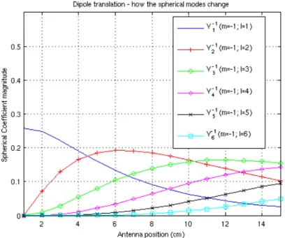
Both translational and rotational operations involving spherical harmonics require the use of the ladder operators ( [20]). These operators are called "ladder" due to the fact that their usage upon a single spherical harmonics induces changes over other spherical harmonics. If we rotate a radiation pattern of a single spherical harmonic of a certain orderL, changes will happen on all modesm inside its specific order. If we translate it, the changes will be on all ordersL, but only for the same originalm.

In fact, translation and rotation of patterns may be responsible for creating new spherical modes, that is how all the spatial diversity is created (and seen) in the domain of spherical harmonics. In the next chapter, it will be shown that the pattern correlation between two antennas can completely calculated only by correlation of their spherical harmonics coefficients. Due to the spatial orthogonality of the spherical harmonics, antennas will be more correlated (lower diversity) as long as they share more coefficients. For this reason, in realistic systems their finite precision is responsible for a trade-off between spatial diversity and computational costs. The greater the number of spherical harmonics, the greater possible diversity, but consequently more required memory to store the antenna coefficients and more complex models. However, some results in this work show that it is possible to obtain a proper balance in this matter.

The translated coefficients _A¯m

l are obtained by the next equation. It is important to

remember that all coefficients must be recalculated after a rotation or translation of the pattern, and not only the originals different than zero.

¯

Aml =Aml (x0+ ∆) =

X

l′_,m′

(−1)l′Aml (x0)Rl∗−l′_,m₋_m′(∆) (2.13)

Rml (x) = (−1)m

1 (l+m)!||x||

l_Ym

l (θ, φ), (2.14)

whereAl,m(x0)is the original coefficient, and∆is the translated distance in meters.

As an example, for an ideal half-wave dipole antenna (assuming that only the modeY1−1 is

(27)

2.3. Tensor decompositions 26

Figure 2.2:Spherical harmonics coefficientsversustranslation. A dipole example

2.2.2 Pattern rotation

According to [20], [21] and [4], any rotation of the spherical harmonics can be done by resorting to Euler rotation angles. In other words, the pattern can be rotated firstly around the z-axis (αangle), then around the y-axis (β angle), and finally around the z-axis again (δ

angle). Thus, using the Wigner-D function ( [9]), the rotated coefficients_Aˇm

l are given by:

ˇ Aml =

l

X

m′=−l

D_mml ′(α, β, δ)A

m′

l , (2.15)

where

D_mml ′(α, β, δ) =e−jmαdl_mm′e−jm ′

δ_, _(2.16)

and

dl_mm′ = (−1)l+m p

(l+m)!(l−m)!(l+m′_)!(_l₋_m′_)!X

k

(−1)k cos

2k−m−m′₍β

2)sin2l+m+m

′ −2k₍β

2) k!(l+m−k)!(l+m′

−k)!(k−m−m′_)!. (2.17) Assuming only a rotation around the z-axis (β = 0andδ= 0), thenDl

mm′ = 0∀m6=m

′ , and all we need to do is to add a phase shift to the spherical harmonics coefficients. Thus, Am l

after rotation in azimuth turns to:

ˇ

Aml =Aml e−jmα. (2.18)

2.3 Tensor decompositions

Over the last years the interest in tensors decompositions has increased exponentially. Originally from the psychology analysis, the tensor decompositions are in frequent use today in a variety of fields ranging from chemometrics, signal processing, bioinformatics, neuroscience, among others ( [22]).

(28)

Model name Decomposition Uniqueness

PARAFAC Xi,j,k=PdAi,dBj,dCk,d Yes

Tucker3 Xi,j,k=Pl,m,nGl,m,nAi,lBj,mCk,n No

Tucker2 Xi,j,k=P_lmGl,m,kAi,lBj,m No

PARATUCK2 Xi,j,k=P_d,eAi,dRd,kGd,eSe,kBj,e Yes†

Table 2.1:Tensor decompositions

own properties formed by specific interactions among their components. See ( [15], [17], [23]) for a more formal definition.

In fact, in MIMO wireless communications, usually tensors are used to expand the channel matrix and/or received signal vector by associating to them other particular types of variations. These new variations correspond to other forms of explorable diversities, such polarization, frequency and time. In Figure 2.3 (left side) it is illustrated receive vectors are grouped to form a tensor that accounts the spatial (i.e. antennas), time (e.g. data-blocks) and code diversities (e.g. CDMA scheme). In the right side of same Figure, the channel tensor is sliced in the frequency dimension.

Space

Time

y

Code

Frequency

Transmit antennas

H

Receive antennas

_{Receive signal} _{MIMO channel}

Figure 2.3: Communications’ tensors. Receive signal and channel

It is worth noting that a model of communications employing both tensors of the Figure 2.3 needs auxiliary structures (e.g. pre-coding matrix) to match the dimensions. This need for auxiliary elements clarifies the idea that different schemes of communications may require different tensor decompositions. Without going further into possible transmission schemes, the well-known tensors decompositions Tucker3, Tucker2, PARAFAC and PARATUCK2 are given in their scalar form expressions in Table2.1.

In the context of wireless communications, the use of tensor modeling in signal processing benefits traditional applications like channel estimation and equalization by exploring multiple (more than two) forms of diversity. As a consequence, estimation of parameters using tensors tend to be less restrictive on the matter of the uniqueness of the solution than matrix-based approaches. In Chapter 4 it is seen a MUSIC-like method using tensors to estimate directions of arrival and departure even if the number of multipaths are greater than the number of antennas. Although this achievement is found in techniques such R-D ESPRIT ( [24]) and Closed-Form PARAFAC based Parameter Estimation (CFP-PE) ( [25]), our method does not need any constraints of array shift-invariance or omnidirectional sensing pattern or only-azimuth directions.

(29)

Parallel Factor Analysis (PARAFAC), also known as Canonical Decomposition (CANDECOMP)( [15], [16], [18]). In this Fundaments Section these two decompositions and the PARATUCK2 one are briefly presented. Their scalar equations are shown in Table2.1.

2.3.1 Tucker

In the third-order Tucker3 decomposition, a core tensorGcombines all columns of matrices A,BandCto compose each element ofX. Due to its great flexibility, the Tucker3 model has rotational freedom, and hence not present the uniqueness property as the PARAFAC model, which may be crucial for many applications. However, particularized additional constraints of specific problems may lead to unique solutions.

The Tucker3 decomposition form is presented in Figure2.4. The Tucker2 decomposition seen in the Table2.1 is a special cases of the Tucker3 decomposition. Note that the Tucker2 decomposition is simpler than its Tucker3 equivalent, since the number of outer product terms has been reduced. A Tucker2 decomposition also arises from a Tucker3 one when one of the factor matrices, sayC, is equal to the identity matrix.

= I

J K

A

M

J

B

K

N

C

L

M N

X

G

L I

Figure 2.4:Tucker model

2.3.2 PARAFAC

The PARAFAC model (Fig. 2.5) ( [15], [16]) can be considered as a special case of the Tucker decomposition where the size of each dimension of the core tensor G is the same (D=L=M =N), and interactions only exist between columns of same indices, such that the only nonzero elements ofGare found along its main diagonal of the core.

The most important feature of the PARAFAC decomposition is its intrinsic uniqueness. In contrast to matrix decompositions, where there is the problem of rotational freedom, the PARARAC decomposition of higher-order tensors is essentially unique, up to scaling and permutation of the columns of its elements. The uniqueness condition is also known as Kruskal’s condition ( [17], [23], [26]). In the Chapter 4 it is shown the Kruskal’s condition to assure uniqueness when estimating directions of arrival and departure.

2.3.3 PARATUCK2

(30)

= I

J K

A

D

J

B

K

D

C

D

D D

X

G

D I

Figure 2.5: PARAFAC model

Being halfway between the Tucker and the PARAFAC decompositions, one can imagine that the core tensor G of PARATUCK2 may have some non-zero elements outside of its main diagonal. A clearer view of this decompositions is possible by observing its graphical representation in Figure2.6, where the core tensorGis replaced by a product of a core matrix Gand two superdiagonal tensorsD(S)andD(R). For these two tensors, the diagonal elements of thek-th slice is built with thek-th of the matricesSorR.

=

I

J K

I D

K

A

T

x D(R)

G

D

D E

E E

E

J

D

K

B

D(S)

Figure 2.6:PARATUCK2 model

(31)

Chapter

3 Analysis of Directional MIMO

Channels Using Spherical

Harmonics Expansion

3.1 Introduction

This chapter deals with the modeling of a MIMO channel matrix using spherical harmonics. The decomposition of a MIMO channel using series of spherical harmonics have been addressed recently in a few works ( [5], [7], [27]). The approach consists in using a spherical harmonic representation of the wavefields so that the MIMO channel matrix is decomposed into the product of known and random matrices where the known portion shows the effects of the physical configuration of antenna elements.

The presence of spherical harmonics in MIMO channels basically started in ( [5]), where it is used for a stochastic modeling of the fading channel coefficients by assuming an uniform distribution of far-field scatterers. In ( [7]), the decomposition of the channel using spherical harmonics already carried information about the effect of scattering clusters distribution. In a recent work [27], the authors have evaluated the impact of the expansion order on the capacity of MIMO antenna systems using patch antenna arrays at both the transmitter and receiver. However, none of this work have used a common model.

3.2 Plane wave representation for an antenna

Given a plane wave arriving at an antenna surrounded by an imaginary sphere of radiusr, the intensity of the field (e.g. electric field) over the sphere’s surface is given by

E(θ, φ) =E0eikTr_, _(3.1)

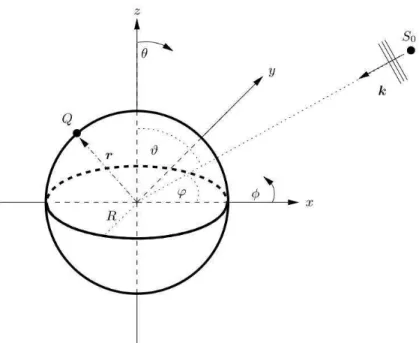
wherek is the wave-vector in a point of the surface, andr is an arbitrary observation point related to the origin of the sphere, as can be seen in Figure3.1( [28]).

(32)

3.2. Plane wave representation for an antenna 31

Figure 3.1:Imaginary sphere surrounding an antenna.

angles for a observation pointQ, we can respectively definekandras:

k=k

   

sen(ϑ)cos(ϕ) sen(ϑ)sen(ϕ)

cos(ϑ)

   

, (3.2)

r=r

   

sen(θ)cos(φ) sen(θ)sen(φ)

cos(θ)

   

. (3.3)

It is noteworthy thatris a function of the surface involving the array, whilekis a function of the well-known wave number (k=||k||= 2πf /c). Combining (3.2) and (3.3), we get:

kTr=kr[sen(θ)sen(ϑ)cos(φ−ϕ) +cos(θ)cos(ϑ)]. (3.4)

The following Section uses spherical harmonics expansion to model the plane wave in Eq. (3.1), as well as to model directional MIMO channels.

3.2.1 Spatial product of two functions in the spherical harmonics domain

Let two fieldsEa(θ, φ)andEb(θ, φ)be represented by their spherical harmonics expansions

according to ( [7], [28],):

Ea(θ, φ) =

√

4π

Lr

X

l=0

l

X

m=−l

Am

l Ylm(θ, φ), (3.5)

Eb(θ, φ) =

√

4π

Lt

X

l=0

l

X

m=−l

Bm

(33)

3.3. MIMO channel decomposition using spherical harmonics 32

where Lt and Lr are the greatest used orders for representing the functions Ea(θ, φ) and

Eb(θ, φ), respectively. Likewise,Aml and Blmare the spherical harmonics coefficients for each

electric field.

Collecting the coefficients and the spherical harmonics in vectors, we get:

a= [A00 A−11 A01 A11 A−22 ... A

Lr

Lr]∈C

1×(Lr+1)2_, (3.7)

b= [B00 B1−1 B01 B11 B−22 ... B

Lt Lt]∈

C1×(Lt+1)2_, (3.8)

yr(θ, φ) = [Y00(θr,1, φr,1) Y1−1(θr,2, φr,2) · · · Y_LL_rr(θr,R1, φr,R1)]

T_∈_C(Lr+1)2×1 (3.9)

yt(θ, φ) = [Y00(θt,1, φt,1) Y1−1(θt,2, φt,2) · · · YLLtt(θt,R2, φt,R2)]

T_∈_C(Lt+1)2×1 (3.10)

Thus, omitting the angular arguments, the product of these fields in the same spatial direction is given by

ˆ

H =EaEb, (3.11)

and using (3.7), (3.8), (3.9), and (3.10), we get

ˆ

H =a(yryTt)bT. (3.12)

Therefore, the product of two any functions in the spatial domain translates into the outer product of their associated spherical harmonics expansion vectors.

The next Section will address the modeling of directional MIMO channels using the spherical harmonics expansion model of Eq. (3.12).

3.3 MIMO channel decomposition using spherical harmonics

For the MIMO system shown in Figure 3.2, it is also interesting to picture a imaginary sphere surrounding each array of antennas, where each one of them can be considered as an “observation” point of the incident wave [8]. We consider that each antenna has its own expansion coefficients, once the array’s resultant electric field is a superposition of fields from every radiating element. The concept of sphere is basically associated with the limiting edge between near and far fields, and also intrinsically carries the idea of angular components (θ

andφ) that characterize the Direction of Arrival (DoA) and Direction of Departure (DoD). The surrounding sphere also establishes a link between the spatial information of the environment (channel) and its spherical harmonics expansion.

Assuming that all incident waves impinging on the array are scattered multipath waves (without line of sight component), the total gain of all waves travelling from theq-th transmit antenna to thep-th receive antenna is given by

R1 X

r1=0

R2 X

r2=0

ˆ

H(θr,r1, θr,r2) =

R1 X

r1=0

R2 X

r2=0

c(r1, r2)ayr(θt,r1)y T

t(θt,r2)b

T_, _(3.13)

where

(34)

..

.

T

_x 1 2 Q

..

.

1 2 P

R

_x

Figure 3.2:MIMO system withP receive antennas andQtransmit antennas

◮ c(r1, r2)- complex amplitude (gain) of the path linking ther1-th receive cluster to ther2-th

transmit cluster;

◮ yr(θr,r1)∈C

(Lr+1)2 - spherical harmonics basis for_r1-th direction of arrival (_DoA);

◮ y_t(θ_r,r₂)∈C(Lt+1)2 - spherical harmonics basis for_r2-th direction of departure (_DoD;

Let us call H(p, q)the element of the channel matrix H that models the link between the

p-th receive antenna to the q-th transmit antenna. Then, for each transmit-receive antenna pair, we have:

H(p, q) =

R1 X

r1=0

R2 X

r2=0

c(r1, r2)a(p)yr(θr,r1)y T

t(θt,r2)b

T₍_q₎ _(3.14)

= a(p)

"_R₁ X

r1=0

R2 X

r2=0

c(r1, r2)yr(θr,r1)y T

t(θt,r2) #

bT(q) (3.15)

or, compactly,

H(p, q) =a(p)Mb(q)T, (3.16) where

M=

R1 X

r1=0

R2 X

r2=0

c(r1, r2)yr(θr,p1)y T

t(θt,p2)∈C

(Lr+1)2×(Lt+1)2_, (3.17)

denotes the mode-to-mode matrix ( [7], [27], [29]) that maps the Mt = (Lt+ 1)2 transmit

spherical modes intoMr= (Lr+ 1)2 receive spherical modes as a result of wave propagation

through the wireless channel [8].

Thus, by capitalizing on the spherical harmonics expansion, we can decouple the response of each transmit and receive antenna from that of the MIMO propagation environment as shown in (3.16). Specifically, by means of this decomposition, the effective MIMO channel is now divided into three parts: transmit side, propagation (physical) channel, and receive side.

Defining A=        a(1) a(2) .. . a(P)

      

∈CP×(Lr+1)2_, and _B₌

       b(1) b(2) .. . b(Q)

      

(35)

the overall MIMO channelH_∈CP×Q admits the following bilinear decomposition:

H=AMBT. (3.19)

Note that in (3.19), the transmit and receive antenna array responses are decoupled from the channel response in the modal (spherical expansion) domain. In contrast to conventional MIMO channel modeling approaches, the spherical mode decomposition allows only the mode-to-mode matrix to be modeled as a stochastic quantity, while vectors A and B are deterministic quantities only depending on the antenna characteristics. Thus, this MIMO channel model has an inner stochastic part represented by the mode-to-mode matrix and outer deterministic part represented by transmit/receive antenna response matrices.

The orthogonality of spherical modes allows a direct analogy between the channel matrix H and the mode-to-mode matrix M. By decoupling the antennas’ responses from the propagation channel model, we can interpret the matrixMas in inner MIMO communication link within a more global channel that include the effects of the transmit/receive antennas. We can imagine that each spherical harmonics mode represents a virtual antenna (feeded by the real antennas), and then most of the mathematical considerations forH can be applied forM, such the idea of sub-channels, correlation between modes, etc. Possible applications can also be thought of as the multiplexing of information over spherical modes and algorithms like water-filling (leveling the coefficients of each spherical harmonics).

3.3.1 Including polarization information

Including the vertical and horizontal polarizations in the channel representations demands a separation between them, since they represent independent domains. In other words, each antenna has two orthogonal fields (vertical and horizontal), and thus each of both fields has its own set of spherical harmonics coefficients, once we are dealing with scalar spherical harmonics in independent structures, as follows:

Mhh= R1 X

r1=1

R2 X

r2=1

chh(r1, r2)yr(θr,r1)y T

t(θt,r2), (3.20)

Mhv= R1 X

r1=1

R2 X

r2=1

chv(r1, r2)yr(θr,r1)y T

t(θt,r2), (3.21)

Mvh= R1 X

r1=1

R2 X

r2=1

cvh(r1, r2)yr(θr,r1)y T

t(θt,r2), (3.22)

Mvv = R1 X

r1=1

R2 X

r2=1

cvv(r1, r2)yr(θr,r1)y T

t(θt,r2). (3.23) In a case of single-scattering clusters, the the double summation present in each of the previous equations is replaced by a single summation over Nd directions. In this case, the

mode-to-mode matrix can be factored as follows:

Mhh=YrDhhYTt (3.24)

(36)

Mvh=YrDvhYTt (3.26)

Mvv=YrDvvYtT (3.27)

where

Yr=

      

yT₂(1)

yT₂(2)

.. . yT₂(Nd)

       T

∈C(Lr+1)2×Nd_, _Y

t=       

yT_t(1)

yT_t(2)

.. . yT_t(Nd)

      

∈C(Lt+1)2×Nd_, (3.28)

are matrices whose columns collect the spherical mode expansions for each of theNddifferent

DoA and DoD angles, respectively, and

Dxy=

      

cxy(1) 0 · · · 0

0 cxy(2) · · · 0

..

. ... . .. ...

0 0 · · · cxy(Nd)

       (3.29)

contains the cluster gains associated with the polarization pairxy, withxy ∈ {hh, hv, vh, vv}. The formulation presented in equations (3.28)-(3.27) can also be extended to the double-scattering clusters, and will be seen in Chapter 4 in more detail.

When including the polarization, Equation (3.19) gives rise to the following co- and cross-polarized MIMO channels:

Hhh=AhMhhBTh. (3.30)

Hhv=AhMhvBTv. (3.31)

Hvh =AvMvhBTh. (3.32)

Hvv =AvMvvBTv. (3.33)

The subscripts present in the definitions ofHandMdefine the coupling between polarizations seen at the transmitter side (right subscript) and at the receiver side (left subscript). By explicitly modeling the polarization domain, we can evaluate the cross-polarization ratio (XPR) of a given propagation scenario by computing the quantity

XP R=c 2

hv+c2vh

c2

hh+c2vv

. (3.34)

Among the useful aspects of this polarized model, we can highlight, for instance, the design of an antenna array receiver that favors the V-V polarization for one antenna pair, and the H-V polarization for some other pair.

(37)

H=

"

Hhh Hhv

Hvv Hvh

#

∈C2P×2Q_, _(3.35)

This means that one could double themultiplexing gainby exploiting orthogonal polarizations. On the other hand, if the same information is sent by each antenna, the overall channel model reduces to

H=

"

Hhh+Hhv

Hvv+Hvh

#

∈C2P×Q (3.36)

meaning that we can increase thediversity gain by using polarization information.

3.3.2 Including time delay

Now concerning the presence of time delayτ, equations (3.30)-(3.33) turn into the general form

H(τ) =AM(τ)BT, (3.37)

where it is assumed that the antennas’ spherical harmonics coefficients (stored in matricesA andB) do not change as a function of τ, but only the propagation medium (M). Moreover, if the delay parameter is considered small enough, the overall channel can be assumed to be a flat-fading channel.

It is worth noting that in equations (4.10)-(4.13), τ would be an argument of the path gainsC, and not of the spherical basis matrix Yr and Yt, which are dependent only on the

directions of arrival and departure of the traveling waves. Introducing the delay parameter

τ, it is possible to get the power delay profile (PDP) associated with each co/cross-polarized channel, which can be useful in an analysis of the impact of polarization in systems with non-negligible multipath delays. Due to delay, the frequency-response of each elementHpq(ω)

can be found simply by taking the Fourier transform

Hpq(ω) =

Z ∞ −∞

Hpq(τ)e−jωτdω (3.38)

The summary of important features in the model presented in this chapter, which are absent in existing spherical harmonics models [3] are:

◮ Multiple scattering - Any combination of DoA/DoD pair can have its own scattering

profile (e.g. power, delay, polarization, etc.). By setting the values ofc(r1, r2)it is possible to model a number of different finite-scattering scenarios with or without interaction between clusters in different delays and polarizations;

◮ Keyhole effect- ‘If the distance between the transmitter (e.g. base station) and receiver

(e.g. mobile station) is much larger than the transmit and receive scatterer radius, then the aperture between angles of arrival and/or departure is smaller ( [3]). This leads to a situation where the columns ofYr and/orYtare highly correlated, thus reducing the

rank ofH, and consequently lowering channel capacity;

◮ Diffuse multipath components- Diffuse (weak) multipaths can be easily incorporated

into our model by assuming a number of random multipaths distributed around the specular component;

◮ Polarization- Polarization can be fully modeled and exploited by means of a directional

(38)

3.4. Antenna translation and rotation 37

3.4 Antenna translation and rotation

As the present model uses the scalar spherical harmonics, it requires the separation of the field patterns into vertical and horizontal patterns as mentioned above (Eqs.(3.30)-(3.33)). For the sake of dissociation ofA and B from M, any rotation or translation shall be done over the spherical harmonics coefficients, these operations involve the use of the ladder operators ( [20]). For further details, see Chapter 2.

After using the Wigner D-function as the rotation operator (Eqs.(2.15)-(2.18), the coefficients shall be projected onto vertical and horizontal axes. As for the cartesian coordinates, the spherical harmonics coefficients can be projected by means of the rotation matrix as follows:

Am pv,l

Am ph,l

!

= cos(θA) sin(θA) sin(θA) cos(θA)

!

Am v,l

Am h,l

!

, (3.39)

and

Bm pv,l

Bm ph,l

!

= cos(θB) sin(θB) sin(θB) cos(θB)

!

Bm v,l

Bm h,l

!

, (3.40)

whereAm

ph,l andAmpv,l are the projected horizontal and vertical components, respectively, and

θAandθB are the rotation elevation angles associated with the receive and transmit patterns,

respectively.

Put it simply, the explicit function of any MIMO channel (Eqs.3.30-3.33) with the previous assumptions is given by

H(τ, θA, θB) =A(θA)M(τ)B(θB)T. (3.41)

The next Section will present the metrics of capacity and correlations. For readability, notations of polarization, rotation and time delay will be omitted. However, it is easy to transport them from the above equations to the next ones.

3.5 Capacity and correlation for MIMO systems

3.5.1 Capacity

Capacity formulae for delay-independent (3.35) and discrete-delay (3.38) channels (omittingθA andθB), respectively, are given by

C=log₂det

IQ+

SN R

Q HH

H _(3.42)

and

C= 1 Nω

Nω

X

n=1

log₂det

IQ+

SN R

Q H[ωn]H[ωn]

H_, _(3.43)

whereNω is the number of evaluated discrete frequencies. 3.5.2 Pattern correlation and subchannel correlation

MIMO channel modeling and estimation: application of spherical harmonics and tensor

MIMO Channel Modeling and Estimation:

Application of Spherical Harmonics and Tensor

Decompositions

LEANDRO RONCHINI XIMENES

MIMO CHANNEL MODELING AND ESTIMATION:

APPLICATION OF SPHERICAL HARMONICS AND

TENSOR DECOMPOSITIONS

Abstract

I

Resumo

Dedicatories

Acknowledgements

List of Symbols

Notation

Contents

List of Figures

List of Tables

Chapter

1

Introduction

1.1 Work context and proposal

1.2 Summary of contributions

1.3 Organization

1.4 Publications

Chapter

2

Fundamentals: Channel models,

Spherical harmonics and Tensors

2.1 Channel models

2.2 Spherical harmonics

|m|=0 |m|=1 |m|=2

|m|=3 |m|=4

L=1

L=2

L=3

L=4

2.3 Tensor decompositions

X

G

X

Chapter

3

Analysis of Directional MIMO

Channels Using Spherical

Harmonics Expansion

3.1 Introduction

3.2 Plane wave representation for an antenna

3.3 MIMO channel decomposition using spherical harmonics

..

.

T

..

.

R

3.4 Antenna translation and rotation

3.5 Capacity and correlation for MIMO systems