APPLICATION OF ALTERNATIVE REGRESSION
MODELS TO DEAL WITH PROPORTIONS AS
DEPENDENT VARIABLES
José Lourenço Pires Marques
Projecto de Mestrado em Finanças
Orientador:
Prof. Doutor José Dias Curto, Professor Assistente, ISCTE-IUL Business School, Departamento de Métodos Quantitativos
II Abstract
The main purpose of this thesis is to consider different approaches to deal with proportions as dependent variables in regression models.
The Classical Linear Regression Model (CLRM) is the approach that most researchers apply to their data. However, the CLRM is inappropriate to deal with bounded variables whose response is restricted into the interval (0, 1) as dependent variables since it may possibly yield fitted values for the variable of interest that surpass its lower and upper limits.
Due to the CLRM weaknesses, in this thesis we will consider some alternative parametric regression models that include the additive logistic normal distribution, the censored normal distribution, the Beta distribution and the normal distribution with nonlinear response function. A quasi-parametric regression approach will also be considered.
In the empirical case we consider a dataset with financial information from US firms. The dependent variable of the models we intend to estimate is the debt to maturity, which is measured as a proportion of the total debt of the firm that has a maturity larger than three years. The explanatory variables are the abnormal earnings, the asset maturity and the size of the firm.
To compare the above models will be used the Akaike’s information criterion (AIC) and Schwarz criterion (SBC). The distribution that displays the lowest values on both criteria is the best to study proportions as dependent variables. We will also study the adjusted value of each model.
JEL Classification: C10, C16
Keywords: Proportions, dependent variables, alternative parametric and
III Resumo
Com esta tese pretendem-se considerar vários modelos de regressão alternativos ao lidar com proporções, enquanto variáveis dependentes num modelo de regressão.
O método mais utilizado pelos investigadores é o modelo clássico de regressão linear. Contudo, esta não é a abordagem mais indicada para a análise de rácios ou proporções contidas no intervalo (0, 1) enquanto variáveis dependentes, pois os valores gerados por este método tendem a ultrapassar esses limites. Deste modo, serão apresentados como alternativas alguns modelos de regressão paramétricos, que incluem a distribuição aditiva logística normal, a distribuição censurada, a distribuição Beta e a distribuição normal com uma função de resposta não-linear. Será também apresentado um modelo de regressão quase-paramétrico.
No caso empírico consideramos uma base de dados com informação financeira de empresas norte-americanas. A variável dependente dos modelos que pretendemos estudar é a maturidade da dívida, que é medida como a proporção da dívida total da empresa com prazo superior a três anos. As variáveis explicativas destes modelos são os ganhos anormais, a dimensão da empresa e a maturidade do activo.
Na comparação dos modelos irão ser utilizados os critérios de informação de Akaike e de Schwarz. O modelo que apresentar menores valores em ambos os critérios é o que melhor lida com proporções enquanto variáveis dependentes. Também faremos uma breve análise ao valor do (R-quadrado) ajustado de cada modelo.
Classificação JEL: C10, C16
Palavras-chave: Variáveis dependentes, proporções, modelos de regressão alternativos
IV Acknowledgements
I would like to thank my supervisor Professor José Dias Curto, for all the help and patience throughout the development of my master thesis. His comments and availability were appreciated.
I would also like to thank three of my best friends, Carlos, Cláudia and Gonçalo for their helpful contribution, essentially for the ideas and comments they gave me all the way through this effort.
The utmost thanks go to my parents and grandmother that have been behind me although living abroad. Their continuous supports during good and bad times were crucial for me to finish my thesis on time.
V Contents: Abstract ... II Resumo ... III Acknowledgements ... IV 1. Sumário Executivo ... 1 2. Introduction ... 2 3. Literature Review ... 5
3.1 Parametric regression models ... 6
3.1.1 The Normal distribution: a linear response function ... 6
3.1.2 The Additive Logistic normal distribution ... 6
3.1.3 The Censored normal distribution ... 7
3.1.4 The Normal distribution: a nonlinear response function ... 8
3.1.5 The Beta distribution ... 8
3.2 The Quasi-Parametric approach... 11
4. Our Methodology ... 13
4.1 Reference to theoretical studies ... 13
4.1.1 The irrelevant hypothesis ... 13
4.1.2 “Matching” between debt maturity and asset maturity ... 14
4.1.3 Agency costs ... 14
4.1.4 Credit and liquidity risk ... 15
4.1.5 Asymmetric information and signalling ... 16
4.2 Data sample ... 16
4.3 Variables description ... 17
5. Our Empirical Application ... 17
5.1 Analysis of the variables ... 18
5.2 Comparison of the models ... 22
6. Conclusions ... 25
7. References ... 26
1 1. Sumário Executivo
O objectivo desta tese é aplicar modelos de regressão alternativos ao lidar com proporções, enquanto variáveis dependentes num modelo de regressão.
O método mais utilizado pelos investigadores é o modelo clássico de regressão linear. Contudo, este método não é o mais indicado para analisar rácios ou proporções contidos no intervalo (0, 1), enquanto variáveis dependentes pois surgem problemas. Para os ultrapassar serão apresentados modelos de regressão alternativos, os quais se dividem em modelos de regressão paramétricos e modelos de regressão não-paramétricos. Os modelos de regressão paramétricos propostos incluem a distribuição aditiva logística normal, a distribuição censurada, a distribuição Beta e a distribuição normal com uma função de resposta não-linear. Também será também apresentado um modelo de regressão quase-paramétrico.
Estes modelos serão aplicados a uma base de dados com informação financeira de empresas norte-americanas, cuja variável dependente é a maturidade da dívida, que é medida como a proporção da dívida total da empresa com prazo superior a três anos. As variáveis explicativas são os ganhos anormais, a dimensão da empresa e a maturidade do activo.
Serão apresentadas algumas teorias (as mais importantes) relativas à escolha da maturidade da dívida, nomeadamente a teoria dos custos de agência, a teoria da hipótese irrelevante, a teoria da informação assimétrica, a teoria do crédito e risco de liquidez e a teoria da correspondência entre a maturidade do activo e do passivo. Os resultados irão estar de acordo ou não com estas teorias.
Para comparar os modelos de regressão referidos serão utilizados os critérios de informação de Akaike e de Schwarz. Iremos demonstrar que o modelo clássico de regressão linear, apesar dos problemas que revela, é o que melhor lida com proporções enquanto variáveis dependentes num modelo, pois é o modelo que apresenta menores valores em ambos os critérios. Analisando o valor do (R-quadrado) ajustado de cada modelo obtemos a mesma conclusão. Para obter os valores dos critérios (e também do ajustado) utilizámos o comando “program” do programa EViews, especificando a função de verosimilhança de cada modelo e também as fórmulas dos critérios que servem para comparar os modelos.
2 2. Introduction
The main purpose of this thesis is to consider different approaches to deal with proportions as dependent variables in regression models. Besides the Classical Linear Regression Model (CLRM), which is the usual procedure, we will discuss some alternative parametric regression models that are based on the additive logistic normal distribution, the censored normal distribution, the Beta distribution and the normal distribution with nonlinear response function. A quasi-parametric regression approach will also be presented.
In the empirical application we consider a dataset with financial information from 1158 US firms. The dependent variable of the models we intend to estimate is the debt to maturity, which is measured as a proportion of the total debt of the firm that has a maturity larger than three years. The explanatory variables are the abnormal earnings, the asset maturity and the firm size.
To compare the above models will be used the Akaike’s information criterion (AIC) and Schwarz Criterion (SBC). The best distribution is the one that displays the lowest values according to both criteria.
The CLRM which is the common approach to deal with proportions in empirical finance as dependent variables can be defined as follows:
, (1)
where is the dependent variable, x is a vector of explanatory variables
with as a vector of ones, and is a vector of parameters. The
term is a random variable with a certain probability distribution and is called error,
disturbance or stochastic term. It is a combination of four different effects: represents all the independent variables not included in the model; captures possible nonlinearities between and ; absorbs the measurement errors of the variables and ; reflects the unpredictable effects or the stochastic component that affect the model. Index i represents a “typical observation” of cross section data (as is our case), and the time in time series data, the reason why i is replaced by t in the case of temporal data.
Three main assumptions are considered in the ordinary least squares (OLS) estimation process: the conditional normal distribution of the dependent variable
3 , the homoskedasticity nature of the errors and the linearity of the conditional expectation function . According to Kieschnick and
McCullough (2003), the upward CLRM does not provide the best description of because when the dependent variable is bounded between 0 and 1, our three main assumptions are violated. First, proportions are not normally distributed for the reason that they are not defined over R, the usual distribution domain. Second, while the proportions are only observed over a limited domain, the effect of any particular explanatory variable cannot be constant in the whole range of x (except if the range
of is very restricted). To surpass this problem, the conditional expectation should be
a nonlinear function of x, but there is no certainty that the fitted values are within the unit interval. Lastly, the conditional variance is not constant and it must be a function of the mean (the variance will come close to zero as the mean approaches either boundary points). Therefore, the drawbacks of linear model when the dependent variable is a proportion are equivalent to those of the linear probability model for binary data (Papke and Wooldrige, 1996).
The alternative parametric models that we will discuss involve the additive logistic normal distribution, the censored normal distribution, the Beta distribution and the normal distribution with nonlinear response function. We will also consider a quasi-parametric regression model.
The model using the additive logistic normal distribution involves a transformation of the dependent variable, if it is a proportion, to overcome the weaknesses of the CLRM. The logit transformation is the common solution and it is used in fitting the data with a linear response of the transformed dependent variable, using the method of least squares. In spite of its strength, this method has some drawbacks when the dependent variable is a proportion as pointed out by Ferrari and Cribari-Nieto (2004).
The first difficulty is that if assumes the values 0 or 1 it is necessary to perform an adjustment before computing the log-odds ratio because z is not defined in that case, as happens to be defined as . The second problem is that logit is always the assumed link function and as Cox (1996) demonstrated, both link and variance functions should be chosen considering the type of data. The third difficulty is that it is not easy to explain the parameters of the model in terms of the initial response. The fourth drawback is the assumption of the stabilization of the
4 conditional variance. Lastly, proportions generally present asymmetry. According to Aitchison (1986), the dependent transformed variable z is normally distributed
, only if itself follows an additive logistic normal distribution.
An alternative solution to overcome these difficulties is to assume a particular distribution for depending on x, and to estimate the parameters of the conditional
distribution by maximum likelihood. The Beta distribution is very versatile for modeling proportions since its density can have quite different shapes, depending on the values of the two parameters that characterize the distribution (p and q).
Another alternative is to fit a nonlinear regression model to the data modelling the conditional expectation function involving the cumulative logistic function (Cox, 1996), because it allows one to focus on the effect of distributional assumptions, as Kieschnick and McCullough (2003) have pointed out. In this method the estimation is performed through the maximum likelihood method.
Another alternative, the censored normal distribution, or Tobit model, displays some drawbacks when it examines the conditional expectation of a proportion observed over the interval (0, 1). Firstly, it assumes that is normally distributed, but unlike in the case of the normal distribution, its distribution is not defined for values outside the [0,1] interval. Secondly, in that interval the Tobit regression is observationally equivalent to the normal regression model and is subject to the same criticism as the normal regression model.
Cox (1996) and Papke and Wooldridge (1996) introduced a quasi-parametric approach that only defines the first and second moments of the conditional distribution, without specifying the full distribution. The robust methods of this approach are obtained by the expansion of the generalized linear models (GLM) literature from statistics, and the quasi-likelihood literature from econometrics. These robust methods nest the logit or probit function in a more general functional form. Compared with log-odds type procedures, there is no problem in recovering the regression function for the fractional variable and there is no need of further transformations to deal with data at the extreme values of zero and unity, as pointed by Papke and Wooldridge (1996). These functional forms surpass the problems of the Beta distribution and the parameters are estimated by using a Bernoulli quasi-likelihood specification.
These briefly presented models will be discussed in more detail in the next section, which will be the literature review (2). In the section entitled methodology (3) the theories that support the debt maturity model of the empirical application are
5 presented. In the same section they are also described the variables of the model and is given a brief explanation of the criteria used to compare the distributions. The empirical application is presented in the fourth section (4), while in the fifth section appear the most important conclusions (5). The appendices are in the final section (7) of this thesis.
3. Literature Review
In this section we refer the theoretical and empirical work we find relevant dealing with regression models where the dependent variable is a proportion. The two-parameter Beta distribution is the most common distribution for fitting the proportional data. Cribari-Nieto (2004), Kieschnick and McCullough (2003) and other authors also compared this approach with other distributional assumptions. Therefore, this procedure has the largest empirical support
In accordance to Kieschnick and McCullough (2003) proportional data can be classified in four distributional categories: the first one comprises proportions on the open interval (0, 1); the second one includes the proportions observed on the closed interval [0, 1]; the third one refers to vectors of proportion, which are not boundary observations (0's and 1's); and finally the fourth category comprises vectors of proportions, in which some are boundary observations. In this thesis we concentrate on the first two categories and to deal with this kind of data the models can be divided in two main groups: parametric regression models (2.1) and quasi-parametric regression models (2.2). Next we will describe the most commonly used methods in each of these categories.
Kieschnick and McCullough (2003) investigated the alternative regression models for proportions and their maintained assumptions. They organized the results taking into account the likelihood principle perspective which implies that
and , where is a function of a vector of the exogenous variables and is the joint distribution of and . They proceeded to make distinction
between parametric and quasi-parametric specifications of following what other researchers assumed for and and presented five parametric regression models, ordered by frequency of use. These authors also make use of the quasi-parametric approach of Cox (1996) and Papke and Wooldridge (1996).
6
3.1 Parametric regression models
In this section they will be explained five parametric models based on the following distributions:
Normal distribution: linear response function; Additive logistic normal distribution;
Censored normal distribution;
Normal distribution: nonlinear response function; Beta distribution.
3.1.1 The Normal distribution: a linear response function
According to Kieschnick and McCullough (2003), although the OLS is the most common method to analyze data, it “presents a problem in characterizing these studies, as sometimes the sample sizes were large enough to invoke asymptotic arguments to rationalize less stringent characterizations of their regression models.”
These authors focused on the most stringent characterization, because when the t tests or the F tests are examined, it is implicitly assumed that the conditional distribution is a normal distribution, unless the sample size is large (Godfrey, 1988). Further, some commonly reported tests (namely Breusch-Pagan's test for heteroskedasticity) assume that the conditional distribution is a normal distribution regardless of the sample size. Kieschnick and McCullough (2003) conclude that the studies that make such assumption implicitly assume a conditional normal distribution for their respective regression model ( is . This implies that is the function of the explanatory variables , concluding that the conditional
expectation function is linear.
3.1.2 The Additive Logistic normal distribution
In this distribution the dependent variable is transformed via the so-called logit transformation and then is fitted a linear response function to the transformed dependent variable through the least squares principle (OLS) (Demsetz and Lehn, 1985). The logit regression model appears as follows:
7
(2)
where is the logit transformation of the dependent variable and the parameters are estimated by using the least squares principle (OLS), which allows Webb (1983) and others to assume that is distributed as . Aitchison (1986) shows that follows a normal distribution if follows an
additive logistic normal distribution. Thus, if follows an additive logistic normal distribution, then will be a standard normal random variate.
Following Kieschnick and McCullough (2003), the application of this regression model has two drawbacks. First, it assumes that the link function is the logit. Second, this transformation stabilizes the conditional variance. The second drawback is of a higher concern because alternative distributional models for these data (the Beta distribution as example) imply that such a transformation will not stabilize the variance.
3.1.3 The Censored normal distribution
This model, also called Tobit model, has the following specification:
(3)
and
(4)
where { are assumed as independent and identically distributed variables, drawn from a distribution.
The problems identified in this approach arise when one examines the conditional expected value of a proportion observed over the interval (0, 1). The first problem is related to the assumption that follows a normal distribution, since the observed values belong to a specified range and outside of which they are not even defined. Thus, there is no censoring, and the censored normal model is inappropriate for this data. The second problem is that according to the data observed on the interval (0,
8 1), the Tobit regression model is equivalent to the normal regression model, thereby implying that it is also subject to the problems of the model based on that distribution.
3.1.4 The Normal distribution: a nonlinear response function
This method consists in the fit of a nonlinear regression model. The conditional expectation function is assumed to be the cumulative logistic function (Cox, 1996), because this allows one to focus on the effect of distributional assumptions, as Kieschnick and McCullough (2003) argued. Specifically the model can be defined by:
. (5)
In this equation follows a normal distribution with parameters , with the estimation being performed through the maximum likelihood method.
3.1.5 The Beta distribution
The Beta distribution is very flexible to model proportions since its density can have quite different shapes, depending on the values of the two parameters that characterize the distribution (p and q). This distribution deals well with continuous dependent variables, with an interval-level dependent variable or with a dependent variable bounded between two defined endpoints. For a large number of financial ratios it is reasonable to assume they have these properties, and therefore solely a regression model with a bounded domain Beta distribution is able to consider the natural bounds of several dependent variables.
According to Paolino (2001), another advantage of the Beta distribution is that it recognizes the relationship between the mean and the variance, that may occur in proportions. The author also considers that “when we are dealing with a proportion and the theory calls for heterogeneity, a Beta distribution should be applied instead of the normal distribution. Even in cases where the researcher does not have any theoretical concern with the variance function, the potential for heteroskedasticity should raise concerns with normal-least squares estimates and lead one to consider using a Beta distribution to model the heteroskedasticity.”
Smithson and Verkuilen (2006) consider the analysis of variance (ANOVA) that is robust against violations of assumptions, but this procedure can lead to data misinterpretations when dealing with a bounded scaled variable or a proportion, as is
9 the case. They consider that in the normal-theory regression, there are other solutions to surpass heteroscedasticity as the Huber–White heteroscedasticity-consistent covariance estimator or computationally intensive robust regression techniques, although they are not frequently applied by researchers when the dependent variable is a proportion.
According to Wooldridge (1996), the Beta regression model is particularly handy for bounded variables displaying a skew distribution. However, this has some limitations as well. First, it implies that each value in [0,1] is taken on with a zero probability. Therefore the Beta distribution is difficult to justify when at least some portion of the sample is at the boundary values of zero or one. Second, the estimates of are not robust to distributional failure (Gourieroux et al, 1984). However, the first failure does not seem to be a significant one for the Beta regression since the financial ratios are proportions which vary from 0 to 1, so the extreme values are seldom taken.
The following Beta distribution is assumed in several studies:
, (6)
where and refers to the Beta function, with and as shape parameters. The Beta function can be specified as:
. (7)
In order to define a Beta regression model, McDonald and Xu (1995) follow the same procedure as the user manuals of the program SHAZAM, adopting a linear regression model and assuming the mean as a linear function of the exogenous variables. So, if is distributed as a Beta random variate, then:
. (8)
10 . (9)
The conditional density function can be derived by the replacement of (9) into
(6). The above specification can also be used to derive the log-likelihood function for
the Beta regression model, but Kieschnick and McCullaugh (2003) argue that it does not restrict the range of the conditional mean. SHAZAM does not provide the required restrictions on the values of the exogenous variables hence they cannot produce reliable results and thus, this approach of McDonald and Xu (1995) and SHAZAM is not adequate to define a Beta regression model.
According to Kieschnick and McCullough (2003), the application of the quasi-likelihood framework proposed by Cox (1996) constitutes a better approach:
= . (10)
This author applies the logit link because it restricts the conditional mean of a Beta distributed regression into the interval (0, 1), which is appropriate for this distributional model. The logit link is defined as:
. (11)
With the purpose to derive an estimatable regression model, Kieschnick and McCullough (2003) related the Beta distribution parameters with the link function. Therefore, for the Beta distribution defined in (6):
, (12)
Projecting into q, because this is the shape parameter in the Beta distribution, Kieschnick and McCullough advanced the following expression for q, which is consistent with previous equation (12):
11 Swapping this formula for q in expression (6) the conditional distribution of the Beta distributed random variate can be set as:
= (14)
The maximum likelihood estimation principle should be applied to estimate the effect of the various conditioning variables . Thus estimates of the vector can be obtained by maximizing the implied log-likelihood function in respect to the parameters
and p.
3.2 The Quasi-Parametric approach
Cox (1996) and Papke and Wooldridge (1996) applied a quasi-likelihood approach that only defines the first and second moments of the conditional distribution, without specifying the full distribution, when dealing with proportions as dependent variables.
Cox (1996) examined the application of the logit and of the complementary log-log link functions with canonical and orthogonal specifications for the variance functions, and confirmed that the logit link function associated with the orthogonal variance function were the best combination to analyze his data sets. This combination, that the author called orthogonal pair can be defined by:
, (15)
and
. (16)
Papke and Wooldridge (1996) applied an equivalent approach to regression models with a fractional dependent variable, which do not need data transformations when dealing with the boundary values of zero and unity. These robust methods for estimation and inference with fractional response variables are obtained by the
12 expansion of the generalized linear models (GLM) described in the literature of statistics, and the literature on quasi-likelihood in econometrics. There will be no complications in recovering the regression function for the fractional variable when these robust specification tests (which nest the logit or probit function in a more general functional form) are compared with log-odds type procedures. These functional forms surpass the problems of the Beta distribution and can easily deploy and estimate the parameters, using Bernoulli quasi-likelihood methods.
The authors assume the availability of an independent sequence of observations where and N is the sample size. The asymptotic analysis is developed as . With this assumption, for all i:
. (17)
In this formula corresponds to a cumulative distribution function (cdf), and its two best known examples are the logistic function (logit) defined as:
and the standard normal cumulative distribution function (probit): , where is a cdf. However, is not strictly necessary that
should be a cdf.
In equation (17), β can be estimated by the non-linear least squares method (NLS) because the expression is non-linear in β and that is the main reason why a linear model for or for the log-odds ratio is used in practice. Papke and Wooldridge (1996) also consider heteroscedasticity because does not tend to be constant when . The NLS estimator is not efficient when is not constant, but this model remains interesting because it directly estimates .
Papke and Wooldridge (1996) suggest a quasi-likelihood method like the one presented by Gourieroux, Monfort and Trognon (1984), with the following Bernoulli log-likelihood function:
, (18)
well defined for 0 < G(.) < 1. This approach has some advantages: first, it is slightly more robust in estimating the standard errors; second, the Bernoulli’s log likelihood has an easy maximization; and last, because equation (18) is a member of the linear
13 exponential family (LEF), the quasi-maximum likelihood estimator (QMLE) of , achieved by maximizing the following equation (19) is consistent for , assuming that equation (17) holds.
(19)
The Bernoulli QMLE is consistent and - asymptotically normal regardless of the distribution of conditional on , because can be a discrete variable, a continuous variable or have both features.
After they presented two empirical studies, Kieschnick and McCullough (2003) recommend the use of either a parametric regression model based upon the Beta distribution or the quasi-likelihood regression model of Papke and Wooldrige (1996). Concerning the choice between these two regression models, they recommend the application of parametric regression model, unless the sample size is large enough to justify the asymptotic arguments underlying the quasi-likelihood approach.
4. Our Methodology
In this section we will provide a brief description of some of the most relevant theories about the debt maturity choice, based on the work of Laureano (2009). The model variables are also discussed.
4.1 Reference to theoretical studies
To finance new projects and to maximize their value, a firm must choose between equity and debt, as Modigliani and Miller (1958, 1963) first stated. When a company decides to borrow, using the bank or the market, it must choose the maturity length. The following theories about the debt maturity choice will be described: the irrelevant hypothesis (3.1.1), the “matching” between debt maturity and asset maturity (3.1.2), the agency costs model (3.1.3), the credit and liquidity risk model (3.1.4) and the asymmetric information and signaling model (3.1.5).
4.1.1 The irrelevant hypothesis
Modigliani and Miller (1958) introduced the so-called irrelevant hypothesis, later developed by Stiglitz (1974). They consider that the capital structure and the debt
14 maturity are irrelevant to the firm’s value, in the presence of perfect capital markets. According to Laureano (2009), this perfect markets hypothesis supposes that there are no transaction and agency costs and taxes. It also implies that individuals have homogeneous expectations about future investments and that information is costless and available to all agents equally. Considering that the market value of a company is independent of its capital structure, the decision about the maturity of debt does not cause any change in the company’s value and so, becomes irrelevant.
Stiglitz proposes the irrelevance of debt maturity, assuming the following about the perfect capital markets: existence of a general equilibrium, no bankruptcies, existence of a perfect market for bonds with all maturities and all real decisions are taken by companies. Respecting these conditions, he shows the existence of a different general equilibrium where a company, while altering one or more financing policies, has the same value for all bonds with different maturities and the same firm value.
4.1.2 “Matching” between debt maturity and asset maturity
Grove (1974), Morris (1976) and Myers (1977) were some of the authors that first studied the impact of assets maturity on debt maturity. They considered that companies with the aim of minimizing the risk of owning assets, which produce earnings in different periods than those with debt obligations, try to match their assets maturity with their debt maturity. If the assets have more maturity than the debt, their return may not be sufficient for the debt obligations. The opposite situation (the debt has greater maturity than the assets) is also dangerous, because debt obligations must be fulfilled when the current assets cease to generate return, which leads to new investments, according to Laureano (2009). To reduce these risks, the companies try to synchronize both debt and assets maturities, and according to Myers (1977), this match of the debt payments with the declining value of the assets, will decrease agency costs. Thus, firms with medium and long term assets can have more long-term debt in their capital constitution, since the maturity matching allows firms to extend their debt maturity, avoiding the increase of the agency costs.
4.1.3 Agency costs
The agency costs theory deals with the conflict of interests between two agents, in this case between stockholders and creditors. The agency costs of debt can have influence over the maturity and, following Myers (1977), they may occur in what the
15 author called the under-investment problem. Concretely, when the projects are financed with debt, although they can have positive Net Present Value (NPV), it is possible that the managers will not work with them. This happens in situations where companies have a large debt, with low residual claims, where the investment returns mainly benefit the creditors. Thus, knowing in advance that they will probably not get a fair return, the stockholders decide against future investments, which reduce the growing opportunities of the company. Smith and Warner (1979) conclude that these conflicts occur more often in smaller companies.
Laureano (2009), citing Myers (1977), writes as follows:
“the value of a company is measured by the assets value and by the present value of its growing opportunities. These can be seen as options to follow future investments and if these options are not exercised, they expire and the value of the firm decreases.” Myers proposes a reduction in the debt maturity as a solution to the problem, so that it reaches the maturity before the investment options come. Then, in agreement with Myers and Majluf (1984), Mauer and Ott (2000) and Childs et al. (2005), the long-term debt can be obtained by the constant renewing of the short-term debt. Due to this underinvestment problem, the growing options of a company influence the selection of debt maturity.
4.1.4 Credit and liquidity risk
Every company with debt is at risk of failing to refinance that debt. According to Sarkar (1999), the risk of insolvency may have influence over the debt maturity selection. Against this circumstance, a long-term debt financing may appear preferable. However, some companies have no access to such funding because the return that the investors demand for the long-term risk leads the companies to accept riskier and lower quality projects, according to Stiglitz and Weiss (1981) and Diamond (1991a).
Sharpe (1991) and Titman (1992) are in agreement with Diamond, who states that if the debt holder gets informed about this risk before the debt refinancing date this may lead to the deterioration of financing conditions, or even to the ending of the contract. According to Diamond, liquidity risk is the risk that propels the debt holder to inefficiently liquidate its assets, after being denied access to new debt.
Companies that have favorable inside information concerning its future earnings prefer short-term debt because it allows them to obtain better refinancing conditions. Short-term financing means higher liquidity risk but according to Diamond, companies with better ratings give preference to this short-term debt to achieve a lower liquidity
16 risk. The companies whose rating is lower use preferentially the long-term debt to reduce the rollover risk, while the firms whose rating is very low use a short-term debt because they cannot generate enough cash flow to deal with a long-term debt.
4.1.5 Asymmetric information and signalling
Whenever both parties in a contract have different information it is said that there is asymmetric information. Managers usually have more information about the future financial conditions then future or current creditors. After analyzing the relationship between asymmetric information and projects quality, Flannery (1986) concludes that a firm with favorable private information notes its quality with the issuance of short-term debt. This happens due to the fact that high quality projects are less undervalued in the short-term than in the long-term. Firms with adverse information issue a long-term debt, while firms facing the absence of informational asymmetries do not get influenced in the choice of the debt maturity.
Goswani et al. (1995) introduce a temporal distribution of asymmetric information, which suggests that differences in the degree of asymmetric information in case of short or long-term cash-flows affect the choice of debt maturity. They concluded that companies issue a long term debt, when the asymmetry is related to uncertainties of long-term cash-flows. The short-term debt is issued when companies have asymmetric information, related to short and long-term cash-flows.
4.2 Data sample
As we referred before, the main purpose of this thesis is to estimate and compare alternative regression models when the dependent variable is a proportion. In the empirical application we used a sample with 1158 observations of US firms, taken from COMPUSTAT Industrial Annual database. According to Laureano (2009), who followed Korajczyk and Levy (2003), amongst other authors, the financial firms (SIC1 one digit code 6) and utilities (SIC two digits code 49) are excluded from the sample. These types of companies are excluded due to regulation factors as they tend to have considerable different capital structures than the other companies integrated in the sample.
1
SIC stands for Standard Industrial Classification. A complete codes list can be consulted at
17
4.3 Variables description
The variables used in the empirical application are also found in the work of Laureano (2009) and are presented subsequently. Later we will perform a regression to investigate which variables are statistically significant. Those that will be found to be insignificant will not be considered in the final model, but analyzed in the context of the debt maturity.
The dependent variable is the debt maturity (Debt_maturity), which is measured as a proportion of the firm’s total debt that has a maturity larger than three years. As explanatory or independent variables were chosen the abnormal earnings (Abnormal_earnings), the asset maturity (Asset_maturity) and the firm size (Size).
The future abnormal earnings (Abnormal_earnings) specifically, is a variable used as a proxy for firm quality and similar to previous empirical studies of Barclay and Smith (1995) and of Stohs and Mauer (1996), among others. Laureano measured this variable in time , as the difference in earnings per share between time and , divided by time share price.
Stohs and Mauer (1996) consider as proxies for the asset maturity (Asset_maturity) the properties, plants and equipment for the depreciation and amortization expense ratio.
According to Laureano, the variable firm size (Size) is calculated as the natural logarithm of the book value of assets, inflated into 2004 US dollars using the Consumer Price Index (CPI)2.
5. Our Empirical Application
In this section we will analyze the statistical significance of the variables (4.1), and those that are not statistically significant will not be included in the several regression models that we have before described (subsections 2.1 and 2.2 of this thesis). These models will be compared (4.2) through the Akaike and the Schwarz information criteria. We will also take in consideration the adjusted value given by each specific model.
2 Data obtained from the United States Department of Labor – Bureau of Labor Statistics website:
18
5.1 Analysis of the variables
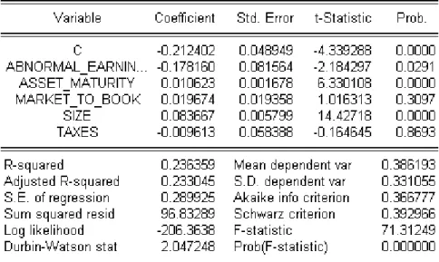
To evaluate the statistical significance of the independent or explanatory variables we will perform a linear regression. Any statistical insignificance of a particular variable will be analyzed in the domain of the debt maturity theories that we already presented, but those variables will not be included in the regression models that we will later estimate. This linear regression is below defined in Figure 1.
Figure 1: Statistical significance of the independent variables
We can attest that the estimated coefficients for the variables Market_to_book and Taxes are not statistically significant because the p-value associated with each one of the t-tests is higher than 0.05 (0.3097 and 0.8693 respectively). The remaining variables (Abnormal_earnings, Asset_maturity and Size of the firm) will be used to explain the dependent variable debt maturity.
Specifically, the variable Market_to_book has a t-statistic of 1.016313 and a
p-value of 0.3097. As it is statistically not significant we cannot conclude anything related
to the agency costs theory. The effective tax rate (Taxes) is affected by the same problem because it is also statistically not significant. Specifically, it has a tstatistic of -0.164645 and a p-value of 0.8693.
19 The coefficient of the log of the firm value (Size) is positive and statistically significant with a t-statistic of 14.42718 and a p-value of 0.0000. This variable has great economic relevance and our results support the credit and liquidity risk theory, in which larger firms tend to have more long-term debt in their capital structure.
According to the signaling hypothesis firms with higher future earnings tend to have more short term debt. Our results sustain this theory because the coefficient of the variable Abnormal_earnings is negative as expected (-0.17816), and statistically significant at the 5% level with a t-statistic value of (-2.184297). It also has a p-value of 0.0291. Therefore, this variable has substantial economic relevance.
The variable Asset_maturity supports the theory relative to the “matching” between debt maturity and asset maturity, because it has a positive coefficient (0.010623), a t-test of 6.330108 and a p-value of 0.00000.
The latter three variables, that are statistically significant, will explain the
Debt_maturity in the models that we have already presented (the additive logistic
normal, the censored normal, the Beta logistic, the normal distribution with nonlinear response function and the quasi-parametric regression models). The parameters of the models are estimated using EVIEWS 5.0-based custom software (shown in Appendices). The general specification of the model is:
.
(20)
The function is in accordance to the specifications that have been considered and explained before. The estimation results are reported in Table 1.
The estimation was performed by the maximization of the likelihood function of each model. Some models require a nonlinear optimization to derive parameters estimates, like the linear censored normal, the transformed logistic normal, the logistic Beta and the quasi-likelihood model. Some models also require initial values for the coefficients of the independent variables, which will not cause interferences in the final estimates. As an example, it is necessary to impute starting values for p in the Beta regression, and for the coefficients mu and sigma in the logistic normal model.
From the analysis of Table 1 we can conclude that the variables asset maturity and size of the firm are statistically significant at the 5% level in every model. Concerning the variable abnormal earnings, some models reject its significance: the
20 transformed logistic normal, the logistic Beta and the quasi-likelihood model. However, this variable is statistically significant at the 5% level in the linear normal model and in the linear censored normal model, and significant at the 10% level in the logistic normal model.
21
Table 1: Estimation results
Linear normal Linear censored normal Transformed logistic normal
Logistic normal
Logistic
Beta Quasi-likelihood model
Estimation method a LS ML LS LS ML QML Constant Coefficient -0.107471 -0.107471 -4528924 -2759409 -2105753 -2715025 SE's b (0.030633) (0.030580) (0.276268) (0.599332) (0.143549) (0.470882) p-values [0.0005] [0.0004] [0.0000] [0.0000} [0.0000] [0.0000] Abnormal_earnings Coefficient -0.153481 -0.153481 -0.374197 -0.684120 -0.429544 -0.719127 SE's (0.076649) (0.076516) (0.691274) (0.400948) (0.297675) -1098385 p-values [0.0455] [0.0449] [0.5884] [0.0880] [0.1490] [0.5127] Size Coefficient 0.073902 0.073902 0.524440 0.336178 0.229339 0.329805 SE's (0.004554) (0.004546) (0.041071) (0.037539) (0.022139) (0.065955) p-values [0.0000] [0.0000] [0.0000] [0.0000] [0.0000] [0.0000] Asset_maturity Coefficient 0.009206 0.009206 0.062959 0.039342 0.026351 0.041405 SE's (0.001572) (0.001569) (0.014178) (0.007415) (0.006991) (0.020329) p-values [0.0000] [0.0000] [0.0000] [0.0000] [0.0002] [0.0417] a
LS, least squares; ML, maximum likelihood; QML, quasi-maximum likelihood b
22
5.2 Comparison of the models
The comparison of models is performed by information criteria, following the principle of parsimony. Thus, the models should adopt a number of parameters as small as possible, because simple models are preferable for two reasons. First, including many variables in the model worsens the relative accuracy of individual coefficients. Second, the resulting loss of degrees of freedom reduces the power of tests performed on the coefficients, increasing the probability of making error type II (not rejecting the hypothesis of nullity of the coefficients when this hypothesis is false).
Simple models are also easier to understand. Thus, these two criteria apply bigger penalties to more complex models and are based on the Residual Sum of Squares (RSS), multiplied by a factor that depends on penalizing model complexity: increased complexity reduces RSS but increases the penalty. A model is preferable to another, if it has less value according to the criteria. The ideal case would be that one model had the lowest value in each of the criteria, but this situation does not always happen.
The RSS can be defined as:
. (21)
The Akaike’s information criterion (AIC) and Schwarz Criterion (SBC) will be the two criteria applied in the comparison of the models. They can be defined as:
, (22)
and
(23)
In both criteria n is the number of observations and k the number of parameters.
The SBC tends to favor simpler models, but penalizes a larger number of coefficients than AIC.
23 An examination of Table 2 allows us to conclude that the linear normal model is the one which has the lowest values in both criteria, AIC and SBC respectively (0.075054 and 0.076376). The logistic normal model and the linear censored normal model also generate acceptable values for both criteria, and close to those of linear normal model.
Looking for the logistic Beta and for the quasi-likelihood model of Wooldridge in Table 2, we obtain different conclusions than Kieschnick and McCullough (2003), who argued that these were the best models for ratios as dependent variables. We can verify that these two models have higher values on both criteria than the linear normal model, the logistic normal and the linear censored normal. For the model based on the additive logistic normal distribution, the transformed logistic normal model, we obtained the same results as Kieschnick and McCullough. Therefore, this model has the highest values in the criteria and so, is the worst in the estimation of proportions.
24
Table 2: Akaike’s information criterion (AIC), Schwarz criterion (SBC) and adjusted
k(x)f( |x) Linear normal Linear censored normal Transformed logistic normal Logistic normal Logistic beta Quasi-likelihood model
AIC 0.075054 0.075237 6.104641 0.075068 1.069737 1.027552 SBC 0.076376 0.076897 6.212159 0.076724 1.093340 1.04565 adjusted R2 0,222540 0,221993 -62,235905 0,222390 -10,071517 -9,644063 ka 3 3 3 5 4 3 R2 0,224556 0,224010 -62,071940 0,225750 -10,033240 -9,616464 a
25 We will still verify if we can come to the same conclusions using the adjusted value as by using the criteria. The adjusted is a modification of that is adapted to the number of explanatory terms in a model. The adjusted can be negative (as is the case), and will always be less than or equal to . The adjusted is defined as:
, (24)
where n is the sample size and k the total number of regressors in the linear model (but not counting the constant term). According to Table 2 the adjusted also considers the linear normal to be the best model since it has the greatest value in this measure (0.222540). This means that 22.254% of the variance of the dependent variable is explained by the model. This measure also considers the logistic normal the second best model (0.222390), closely followed by the linear censored model (0.221993).
The adjusted takes negative results for the other regression models as well. This means that the respective models do not adequately describe the data.
6. Conclusions
In this thesis we considered different approaches to deal with proportions as dependent variables in regression models because the usual method, the CLRM, displays some drawbacks when dealing with fractional dependent variables.
Thus, we studied the application of this and other five regression models (the linear censored normal, the transformed logistic normal, the logistic normal, the logistic beta and a quasi-likelihood model) to examine which one better describes the data. We used two criteria to compare the models, the Akaike’s information criterion and the Schwarz criterion. Based on these two criteria, we concluded that the CLRM even with its own drawbacks is the best model to deal with proportions as dependent variables.
Relatively to the limitations of the study and future investigation, we identified a limitation in this thesis. As in the data set we had several observations with value 0 it was necessary to transform them (we considered a value near zero) in order to apply some of the models under analysis. In future research, as our empirical results are not in accordance to those of Kieschnick and McCullough (2003), it becomes necessary to
26 develop an theoretical (and not just in empirical terms) econometric issue that allows us to decide which model works better with proportions as dependent variables.
7. References
Aitchison, J. (1986), The statistical analysis of compositional data, New York, NY: Chapman and Hall.
Barclay, M. and C. Smith (1995), The Maturity Structure of Corporate Debt, The
Journal of Finance 50, Issue 2, 609-631.
Childs, P.D., David C. Mauer and Steven H. Ott (2005), Interactions of corporate financing and investment decisions: The effects of agency conflicts, Journal of
Financial Economics 76, 667-690.
Cox, C. (1996), Nonlinear quasi-likelihood models: applications to continuous proportions, Computational Statistics & Data Analysis 21, 449-461.
Cribari-Neto, F. and S. L. P. Ferrari (2004), Beta Regression for Modelling Rates and Proportions, Working Paper.
Demsetz, H. and K. Lehn (1985). The structure of corporate ownership: causes and consequences, Journal of Political Economy, 93, 1155–77.
Diamond, D. (1991a), Debt Maturity Structure and Liquidity Risk, Quarterly Journal of
Economics 106, Issue 3, 709-737.
Flannery, M. (1986), Asymmetric Information and Risky Debt Maturity Choice, The
Journal of Finance 41, Issue 1, 19-37.
Godfrey, L. (1988), Misspecification tests in econometrics: the Lagrange multiplier
principle and other approaches, New York: Cambridge University Press.
Grove, M. (1974), On “Duration” and the Optimal Maturity Structure of the Balance Sheet, Bell Journal of Economics 5, Issue 2, 696-709.
Kieschnick, R. and B. D. McCullough (2003), Regression analysis of variates observed on (0, 1): percentages, proportions and fractions, Statistical Modelling, Issue 3, 193-213.
Korajczyk, R. and A. Levy (2003), Capital structure choice: macroeconomic conditions and financial constraints, Journal of Financial Economics 68, Issue 1, 75–109.
Laureano, L. M. S. (2009), Essay on Debt Maturity. Ph.D. Thesis, Department of Management, ISCTE-IUL Business School.
Mauer, D. C. and S. H. Ott (2000), Agency Costs, Underinvestment, and Optimal Capital Structure: The Effect of Growth Options to Expand, in M. J. Brennan and L. Trigeorgis, Eds., Project Flexibility, Agency and Competition: New Developments in the
27 McDonald, J. B. and Y. J. Xu (1995), A generalization of the Beta distribution with applications, Journal of Econometrics 66, 133-152.
Modigliani, F. and M. Miller (1958), The Cost of Capital, Corporation Finance and the Theory of Investment, The American Economic Review 48, Issue 3, 261-297.
Modigliani, F. and M. Miller (1963), Corporate Income Taxes and the Cost of Capital,
The American Economic Review 53, Issue 3, 433-443.
Morris, J. (1976), On Corporate Debt Maturity Strategies, The Journal of Finance 31, Issue 1, 29-37.
Myers, S. C. (1977), Determinants of corporate borrowing, Journal of Financial
Economics 5, Issue 2, 147-175.
Myers, S. C. and N. S. Majluf (1984), Corporate Financing and Investment Decisions When Firms Have Information That Investors Do Not Have, Journal of Financial
Economics 13, Issue 2, 187-221.
Paolino, P. (2001), Maximum Likelihood Estimation of Models with Beta-Distributed Dependent Variables, Political Analysis, 9:4, 325-346.
Papke, L. E. and J. M. Wooldridge (1996), Econometric Methods for Fractional Response Variables with an Application to 401(K) Plan Participation Rates, Journal of
Applied Econometrics, Vol. 11, 619-632.
Sarkar, S. (1999), Illiquidity Risk, Project Characteristics, and the Optimal Maturity of Corporate Debt, Journal of Financial Research 22, Issue 3, 353-370.
Sharpe, S. (1991), Credit rationing, concessionary lending and debt maturity, Journal of
Banking and Finance 15, Issue 3, 581-604.
Smith, C. and J. B. Warner (1979), On financial contracting: An analysis of bond covenants, Journal of Financial Economics 7, Issue 2, 117-161.
Smithson, M and J. Verkuilen (2006), A Better Lemon Squeezer? Maximum-Likelihood Regression With Beta-Distributed Dependent Variables, Psychological Methods, Vol. 11, NO.1, 54-71.
Stiglitz, J. (1974), On the Irrelevance of Corporate Financial Policy, American
Economic Review 64, Issue 6, 851-866.
Stiglitz, J. and A. Weiss (1981), Credit Rationing in Markets with Imperfect Information, American Economic Review 71, Issue 3, 393-410.
Stohs, M. and D. Mauer (1996), The Determinants of Corporate Debt Maturity Structure, Journal of Business 69, Issue 3, 279-312.
Titman, S. (1992), Interest Rate Swaps and Corporate Financing Choices, The Journal
of Finance 47, Issue 4, 1503-1516.
Webb G. K. (1983), The economics of cable television, Lexington, MA: Lexington Books.
28 8. Appendices
Program 1: Computation of the regression models
load "c:\tese\database1.wf1"
'Cálculo da Total Sum of Squares (TSS)
series desvdebt_maturity=(debt_maturity-@mean(debt_maturity))^2 scalar TSS=@sum(desvdebt_maturity)
'Linear normal Equation eq1
eq1.ls debt_maturity c abnormal_earnings size asset_maturity eq1.makeresid resols
series res2=resols^2
scalar RSSOLS=@sum(res2) show eq1.output
scalar R2OLS=1-RSSOLS/TSS coef(1) Beta1 = eq1.c(1)
coef(2) Beta2 = eq1.c(2) coef(3) Beta3 = eq1.c(3) coef(4) Beta4 = eq1.c(4) !k=@ncoef !obs=@obssmpl scalar aicols=(rssols/!obs)*@exp((2*(!k)/(!obs))) scalar sbcols=(rssols/!obs)*(!obs)^(!k/!obs) 'quasi-likelihood model logl ll1
ll1.append @logl logl
ll1.append z = Beta1(1) + Beta2(1) * abnormal_earnings + Beta3(1) * size + Beta4(1) * asset_maturity
ll1.append logl = (debt_maturity*((z)-@log(1+@exp(z)))+(1-debt_maturity)*(-@log(1+@exp(z)))) ll1.append resloglike2=(debt_maturity-z)^2 ll1.append RSSLOGLIKE=@sum(resloglike2) ll1.append R2LOGLIKE=1-RSSLOGLIKE/TSS !l=@ncoef ll1.append aicloglike=(rssloglike/!obs)*@exp((2*(!l)/(!obs))) ll1.append sbcloglike=(rssloglike/!obs)*(!obs)^(!l/!obs) ll1.ml(d) show ll1.output
29 'Transformed logistic normal
Equation eq2
eq2.ls @log(debt_maturity/(1-debt_maturity)) c abnormal_earnings size asset_maturity eq2.makeresid restransf series res3=restransf^2 scalar RSSTRANSF=@sum(res3) show eq2.output scalar R2TRANSF=1-RSSTRANSF/TSS !m=@ncoef scalar aictransf=(rsstransf/!obs)*@exp((2*(!m)/(!obs))) scalar sbctransf=(rsstransf/!obs)*(!obs)^(!m/!obs) 'Linear censored normal
Equation eq3
eq3.censored(r=1) debt_maturity c abnormal_earnings size asset_maturity eq3.makeresid rescenso series res4=rescenso^2 scalar RSSCENSO=@sum(res4) show eq3.output scalar R2CENSO=1-RSSCENSO/TSS !n=@ncoef scalar aiccenso=(rsscenso/!obs)*@exp((2*(!n)/(!obs))) scalar sbccenso=(rsscenso/!obs)*(!obs)^(!n/!obs) 'Logistic normal coef(1) sigma=0.5 coef(1) mu=0.5 !pi = @acos(-1) logl ll2
ll2.append @logl logl
ll2.append z = Beta1(1) + Beta2(1) * abnormal_earnings + Beta3(1) * size + Beta4(1) * asset_maturity
ll2.append res = debt_maturity-(1/(1+@exp(-z)))
ll2.append logl = -@log(sigma(1))-0.5*@log(2*!pi)-0.5*((res-mu(1))/sigma(1))^2 ll2.append resnonlin2=res^2 ll2.append RSSNONLIN=@sum(resnonlin2) ll2.append R2Nonlin=1-RSSNONLIN/TSS !o=@ncoef ll2.append aicnonlin=(rssnonlin/!obs)*@exp((2*(!o)/(!obs))) ll2.append sbcnonlin=(rssnonlin/!obs)*(!obs)^(!o/!obs) ll2.ml(d) show ll2.output 'Logistic Beta coef(1) p=0.2 logl ll3
ll3.append @logl logl
ll3.append z = Beta1(1) + Beta2(1) * abnormal_earnings + Beta3(1) * size + Beta4(1) * asset_maturity
30 ll3.append q=p(1)*@exp(-z)
ll3.append logl = @gammalog(p(1)+q)-@gammalog(p(1))-@gammalog(q)+(p(1)-1)*@log(debt_maturity)+(q-1)*@log(1-debt_maturity) ll3.append resBeta2=(debt_maturity-z)^2 ll3.append RSSBETA=@sum(resBeta2) ll3.append R2BETA=1-RSSBETA/TSS !p=@ncoef ll3.append aicBeta=(rssBeta/!obs)*@exp((2*(!p)/(!obs))) ll3.append sbcBeta=(rssBeta/!obs)*(!obs)^(!p/!obs) ll3.ml(d) show ll3.output