Repositório ISCTE-IUL
Deposited in Repositório ISCTE-IUL:2019-03-26
Deposited version:
Post-print
Peer-review status of attached file:
Peer-reviewed
Citation for published item:
Gomes, O., Ferreira-Lopes, A. & Sequeira, T. N. (2014). Exponential discounting bias. Journal of Economics (Zeitschrift für Nationalökonomie) . 113 (1), 31-57
Further information on publisher's website:
10.1007/s00712-013-0363-3
Publisher's copyright statement:
This is the peer reviewed version of the following article: Gomes, O., Ferreira-Lopes, A. & Sequeira, T. N. (2014). Exponential discounting bias. Journal of Economics (Zeitschrift für Nationalökonomie) . 113 (1), 31-57, which has been published in final form at https://dx.doi.org/10.1007/s00712-013-0363-3. This article may be used for non-commercial purposes in accordance with the Publisher's Terms and Conditions for self-archiving.
Use policy
Creative Commons CC BY 4.0
The full-text may be used and/or reproduced, and given to third parties in any format or medium, without prior permission or charge, for personal research or study, educational, or not-for-profit purposes provided that:
• a full bibliographic reference is made to the original source • a link is made to the metadata record in the Repository • the full-text is not changed in any way
The full-text must not be sold in any format or medium without the formal permission of the copyright holders. Serviços de Informação e Documentação, Instituto Universitário de Lisboa (ISCTE-IUL)
Orlando Gomesy Alexandra Ferreira-Lopesz Tiago Neves Sequeirax
July 2012
-Abstract
We address intertemporal utility maximization under a general discount function that nests the exponential discounting and the quasi-hyperbolic discounting cases as particular speci…cations. The suggested framework intends to capture one important anomaly typically found when addressing the way agents discount the future, namely the evidence pointing to the prevalence of decreasing impatience. The referred anom-aly can be perceived as a bias relatively to what would be a benchmark exponential discounting setting, and is modeled as such. The general discounting framework is used to address a standard optimal growth model in discrete time. Transitional dynamics and stability properties of the corresponding dynamic setup are studied. An extension of the standard growth model to the case of habit persistence is also considered.
Keywords: Intertemporal Preferences, Exponential Discounting, Quasi-hyperbolic Discounting, Optimal Growth, Habit Persistence, Transitional Dynamics.
JEL Classi…cation: C61, D91, O41.
We thank participants and organizers of the 6thAnnual Meeting of the Portuguese Economic Journal
and the comments of colleagues from the BRU - IUL Research Unit. Alexandra Ferreira-Lopes and Orlando Gomes acknowledge …nancial support from PEst-OE/EGE/UI0315/2011. Alexandra Ferreira-Lopes and Tiago Neves Sequeira acknowledge support from FCT, Project PTDC/EGE-ECO/102238/2008.
yCorresponding author. Instituto Superior de Contabilidade e Administração de Lisboa
(IS-CAL/IPL) & BRU - IUL (BRU - Business Research Unit). Address: Instituto Superior de Con-tabilidade e Administração de Lisboa (ISCAL/IPL), Av. Miguel Bombarda 20, 1069-035 Lisbon, Portugal. E-mail: [email protected]
zInstituto Universitário de Lisboa (ISCTE - IUL), ISCTE Business School Economics
De-partment, BRU - IUL (BRU - Business Research Unit), and CEFAGE - UBI. E-mail: [email protected].
xManagement and Economics Department, Universidade da Beira Interior (UBI) and
1
Introduction
Typically, the benchmark utility maximization dynamic model takes a constant rate of time discounting and, thus, intertemporal discounting is modeled as being exponential. This is an analytically convenient assumption and it is logically consistent with the idea that a constant interest rate is often used to compare the value of money over time, for instance at the level of the evaluation of investment projects. However, there are psychological e¤ects that must be taken into account when addressing intertemporal preferences. Such e¤ects may have a huge impact on how we perceive the behavior of the representative agent in the context of conventional economic models since they tend to generate a departure relatively to exponential discounting.
In Xia (2011) three types of time preference anomalies that imply a deviation relatively to the standard exponential discounting framework are identi…ed. These relate to the timing of the evaluation, the magnitude of the reward, and the sign of the reward. The sign e¤ect was …rst highlighted by Kahneman and Tversky (1979) and basically states that gains are discounted more than losses. The magnitude e¤ect is a matter that has received increasing attention on recent literature (see Noor, 2011 and Bialaszek and Ostaszewski, 2012) and relates to the evidence that there is an inverse relation between the amount of the reward and the steepness of discounting over time, i.e., agents tend to be more patient when larger rewards are under evaluation.
The most debated issue, though, is the one concerning changes on the degree of im-patience as time elapses. This point relates essentially to the basic evidence that there is decreasing impatience over time – human beings tend to place much more weight on the di¤erence between a reward to be received (or a cost to be incurred) today or tomorrow than on the di¤erence between two consecutive dates in the far future. Thus, the rate of discount that we apply when measuring the present value of some near in time outcome is typically much larger than the discount rate applied to a distant in the future event. This is also the same as saying that the discount rate decreases in time. Such type of phe-nomenon is known as hyperbolic discounting and it has been widely discussed at various levels in recent years.
The discussion on the subject, from an economic point of view, has started with Strotz (1956) and Pollak (1968) and received in‡uential contributions in the 1990s, with the work, among others, of Akerlof (1991), Laibson (1997, 1998) and O’Donoghue and Rabin (1999). These authors have raised some fundamental questions: Does the popularity of exponential discounting come from its time consistency or from analytical tractability? How can one incorporate into economic models an operational notion of decreasing impatience? If preferences are truly present-biased, how does this relate to important behavioral issues as self-control or procrastination? Are agents aware of their own intertemporal preferences, so that they adopt sophisticated plans of action or does unawareness lead to a naive interpretation about the future?
eco-nomics and related …elds. Part of the debate is still centered on justifying why hyperbolic discounting should be considered a rational way to form intertemporal preferences, more than exponential discounting. Prelec (2004), Dimitri (2005), Drouhin (2009), Farmer and Geanakoplos (2009), and Gollier (2010) argue that hyperbolic discounting is time consis-tent and rational. Decreasing impatience in a stochastic environment allows for a formal proof of such claim. Other authors are more skeptical about how hyperbolic discounting is being approached in the literature. While there is a tendency to search for analytical discount functions that may allow for an elegant treatment of economic models, one should take into account arguments as the ones by Rubinstein (2003) and Rasmussen (2008) who believe that modifying functional forms does not answer the main questions posed by the apparent lack of rationality in economic behavior. As stated by Ariel Rubinstein, a deeper understanding of intertemporal human decisions requires opening the black-box of decision making more than changing slightly the structure of the model used to address human behavior.
Other relevant contributions on the …eld of hyperbolic discounting relate the generaliza-tion of the concept and the exploitageneraliza-tion of the corresponding implicageneraliza-tions. In Bleichrodt, Rohde, and Wakker (2009) the commonly used discount functions are modi…ed in order to account for other kinds of time inconsistency on the formation of preferences besides decreasing impatience. Speci…cally, the proposed framework accommodates the possibil-ities of increasing impatience and strongly decreasing impatience. Also Benhabib, Bisin, and Schotter (2010) present a general version of the discount function, that contemplates the most common speci…cations of exponential and hyperbolic discounting found in the literature.
The powerful notion of hyperbolic discounting, and its most common speci…cation in economics - Laibson’s quasi-hyperbolic discounting concept - have been applied to study a wide range of relevant economic issues. Just to cite a few, we highlight the contributions of Gong, Smith, and Zou (2007), concerning consumption under uncertainty, Groom et al. (2005), Dasgupta (2008), Gollier and Weitzman (2010), and Hepburn, Duncan, and Papachristodoulou (2010) in the …eld of environment policy, namely when making the distinction between social and private discount rates, a paramount normative question in this …eld, Graham and Snower (2007) on short-run macroeconomics and in‡ation dynam-ics, and, Barro (1999) and Coury and Dave (2010) on the implications of non-exponential discounting to economic growth.
In this paper we generalize the quasi-hyperbolic discounting setting and apply the new framework of intertemporal preferences to a standard discrete time optimal growth problem. The setup di¤ers from other approaches on the subject because we relate the shape of the discount function to issues of …nancial literacy, following the analysis on the exponential growth bias as developed by Stango and Zinman (2009) and Almenberg and Gerdes (2011). Our argument is that in the same way people tend to underestimate future values of variables that grow at constant rates, individuals also tend to overestimate close in time values (relatively to the ones more distant in the future) when discounting them to
the present. This reasoning allows us to present a discount function that is ‡exible enough to characterize di¤erent degrees of hyperbolic discounting and to nest the exponential discounting case as a possible limit outcome.
The proposed speci…cation of intertemporal preferences is analytically convenient to address a discrete time optimal growth model. It enables us to derive explicit stability conditions and it serves to compare di¤erent degrees of deviation from the constant dis-count rate benchmark. Additionally, we extend the model to include habit persistence in consumption in order to demonstrate the ‡exibility of the exponential discounting bias concept when used in di¤erent settings.
The remainder of the paper is organized as follows. Section 2 discusses in detail the notion of exponential discounting bias relating it with …nancial literacy issues. In section 3 this concept is applied to compare di¤erent possibilities in terms of hyperbolic discounting. Section 4 approaches utility maximization under the general speci…cation for intertemporal preferences. Section 5 sets up the growth model and analyzes the underlying dynamics. In section 6, an extension is explored; namely, the model is adapted in order to account for habit persistence. Finally, section 7 concludes.
2
Anomalies in Financial Evaluation
Recently, Stango and Zinman (2009) and Almenberg and Gerdes (2011) have carefully analyzed the evidence that points to a tendency to underestimate the future value of a given variable that grows at a constant rate. This exponential growth bias clearly exists in practice, for instance in what concerns household …nancial decision making.
The mentioned literature emphasizes the link between the extent of the bias and the degree of …nancial literacy. A poor ability to perform basic calculations and the lack of familiarity with elementary …nancial concepts and products will, in principle, imply a wider gap between individuals’ calculations and the true future values, i.e., there is a negative correlation between …nancial literacy and the exponential growth bias.
Well informed agents will be able to understand the basic notion of capitalization and to perceive the exponential path followed by any value that accumulates over time. However, many studies have been discovering serious ‡aws on the understanding, by the average citizen, of simple …nancial concepts and mechanisms. This was highlighted by Lusardi (2008) and Japelli (2010), among others. Financial literacy or, more precisely, the lack of it, can explain the kind of de…ciency that consists in linearizing an exponential series in time.
The important argument concerning the lack of ability on accurately addressing the value of money in time is that incorrect answers are biased. As emphasized by Almenberg and Gerdes (2011), individuals are almost twice as likely to underestimate the correct amount than to overestimate it. Thus, on the aggregate it makes sense to state that in a society where a given degree of …nancial illiteracy exists, the future values of a series that grows at a constant rate will be underestimated. Exponential growth bias will then be
common when assessing the future value of an investment that o¤ers a return at a given annual constant interest rate.
It is reasonable to conceive the existence of a link between the interest rate and the rate of time preference. In Farmer and Geanakoplos (2009, pages 1,2), this link is explained in simple terms,
’A natural justi…cation for exponential discounting comes from …nancial economics and the opportunity cost of foregoing an investment. A dollar at time s can be placed in the bank to collect interest at rate r, and if the interest rate is constant, it will generate exp(r(t s)) dollars at time t. A dollar at time t is therefore equivalent to exp( r(t s)) dollars at time s. Letting = t s, this motivates the exponential discount function Ds( ) = D( ) = exp( r ), independent of s.’
The above sentence establishes a possible direct connection between the interest rate and the discount rate of intertemporal preferences. Nevertheless, there is a substantial di¤erence between the two. While the interest rate is obtained as a market outcome, and might not vary if market conditions do not change, the rate of intertemporal choice is a matter of perception and preferences. Agents may want to adopt a rate of time preference that is close to the interest rate, but if they fail in understanding how future values accumulate, the lack of …nancial literacy eventually helps in explaining why the subjective rate of time impatience possibly departs from a constant value or, in other words, why discounting possibly deviates from the benchmark exponential case under a constant discount rate.
To understand how …nancial illiteracy might contribute to deviate agents’preferences from exponential discounting, we just need to make the inverse path to the one that is present in the evaluation of the exponential growth bias, i.e., if individuals tend to under-estimate future values when assessing them in the present, they will certainly overunder-estimate current values when thinking about them as if they were taking decisions at some future time moment. In analytical terms, the idea of exponential growth bias is commonly pre-sented as F V = P V (1 + r)(1 )t, where F V is the future value, P V the present value, r the interest rate, t is time and 2 (0; 1) measures the magnitude of the bias. If one wants to address the present value given the future value, we just need to rearrange the previous expression and write it as P V = F V =(1 + r)(1 )t.
The above relation implies decreasing impatience. Far in the future outcomes are much less valued than the ones occurring in the near future. Now the bias works on the opposite direction - near in time results are overestimated. We can call this e¤ect exponential discounting bias, and we may de…ne it as the tendency to overestimate close in time values of a variable that grows at a constant rate.
The exponential discounting bias will be bigger the larger is the extent of …nancial illiteracy and it constitutes an alternative explanation about why preferences in time tend to imply hyperbolic discounting: agents want to select a constant rate of time preference, namely a rate of time preference that follows the interest rate path, but their ability to
undertake the proper computations is biased, in such a way that far in time values are less considered than the ones near the current period.
Taking into consideration the notion of exponential discounting bias can be an ana-lytically convenient way of approaching departures from strict exponential discounting. According to the distinction introduced by O’Donoghue and Rabin (1999) between naive and sophisticated agents, the discussed bias puts us closer to the naive evaluation of intertemporal preferences in Akerlof (1991) than to the sophisticated behavior that is im-plicit in Laibson’s (1997, 1998) analysis. In this context, a sophisticated person will know exactly what the respective future selves’preferences will be, while naive individuals are not able to realize that as time evolves, preferences will evolve as well.
As a result of the understanding that a bias on discounting cannot be perceived by the agent, since it is the outcome of an anomaly on an otherwise intended constant discounting behavior, the representative agent in the models of the following sections will display a clearly naive behavior. Therefore, she will not be concerned with the possibility of tomorrow selves choosing options that are di¤erent from the ones chosen today. Since people are not aware of their own time inconsistency, it is legitimate to consider a dynamic optimal control problem where the representative agent maximizes at a given date t = 0 her future utility, and thus to design an optimal plan where the present bias exists but the agent acts as if it did not exist.
In short, the analysis in this paper …nds support on two logical arguments:
First - Individuals desire to turn intertemporal preferences compatible with the oppor-tunity cost of money. This is the benchmark time consistent behavior that the rational agent would like to adopt;
Second - Lack of a solid …nancial literacy eventually introduces a biased evaluation of intertemporal preferences, that makes the representative agent to act as if she was an exponential discounter, when in fact she is not.
3
Departures from Exponential Discounting
In order to account for decreasing impatience, Loewenstein and Prelec (1992) have pro-posed the following hyperbolic discount function: DH(t) = (1 + t) = , where and are two positive parameters. This discount function implies a decreasing discount rate: short-term discount rates are higher than long-term discount rates. Empirical evidence suggests that this is a much more appropriate and realistic way to approach intertemporal preferences then just considering a constant discount rate over time.
While empirically more suitable, hyperbolic discounting, considered as modeled above, is much less tractable from an analytical point of view than exponential discounting. Be-cause of this, Laibson (1997, 1998), based on a previous formalization by Phelps and Pollak (1968), has proposed an approximation to hyperbolic discounting, that he dubbed quasi-hyperbolic discounting; this is straightforward to apply to the standard dynamic optimization models of economists. The discount function takes the following form:
DQH(t) = (
1 if t = s bbt s
if t = s + 1; s + 2; ::: , with s the time period in which the future is being evaluated; b 2 (0; 1), b 2 (0; 1). Note that in the limit case b = 1 we are back at exponential discounting.
As in the hyperbolic case, the quasi-hyperbolic discount function captures the idea that discount rates decline with the passage of time. Laibson proposes, in his studies, a small exercise to compare discount rates on each of the settings. He considers exponential discounting (b = 1; b = 0:97), quasi-hyperbolic discounting (b = 0:6; b = 0:99), and hyperbolic discounting ( = 105; = 5 103) and draws a graph where it is evident that DQH(t) generates a time trajectory that is considerably closer to DH(t) than the one originating in plain exponential discounting.
In the previous section, it was stated that the absence of a stable impatience level over time may be interpreted as an anomaly, something similar to the tendency that individuals have to linearize a series of values that accumulate at a constant rate (and, hence, truly exhibit an exponential path). In the proposed setting, this anomaly should be considered in the reverse way, i.e., if individuals tend to linearize exponential trajectories for the future, when discounting values to the present they will exacerbate the exponential nature of the series under analysis.
In this context, we will consider exponential discounting, DE(t) = t s, 2 (0; 1), but we add the possibility of an error of evaluation that increases short-run impatience, gen-erating a kind of hyperbolic discounting. Let (t) be the anomaly term, which transforms DE(t) into a discount function with an exponential bias, i.e., DEB(t) = (1+ (t))(t s). Function (t) will take the following form: (t) =
(
0 if t = s
1
t s 0 if t = s + 1; s + 2; ::: . The assumption of DEB(t) as the discount function has two advantages. On one hand, it allows for an intuitive explanation on why we depart from exponential discounting. There is an error of evaluation by the agents; perhaps they want to adopt a constant discount rate but, relatively to the periods that are closer in time they do not have the capacity to make an objective evaluation of their priorities. As time goes by, such ability evolves and, in the long-run, the error in evaluation is much smaller. On the other hand, we introduce a more general and ‡exible approach to time discounting than the one underlying DQH(t); as we will see below, the values of , 0, and 1 can be chosen in such a way that we obtain an approximation to DH(t) that is undoubtedly better than the one provided by quasi-hyperbolic discounting.
We consider 0 2 [0; 1] and 1 0. Naturally, exponential discounting holds for 0 = 1 = 0, while quasi-hyperbolic discounting is also a particular case of the more general setting provided by DEB(t) for b = 1 and b = (1 0). Recover Laibson’s
example and consider the following parameter values for the exponential bias discount function: = 0:97, 0 = 0:95, and 1 = 23. Figure 1 displays a graph that is similar to the one in the original Laibson’s analysis (50 periods are considered and hyperbolic and quasi-hyperbolic discount functions are displayed; pure exponential discounting is ignored
in the displayed …gure). To this …gure, we add the exponential bias case for the parameter values that were chosen.
It is evident that the new function generates results that o¤er a much better …t with the hyperbolic discount function than the ones generated by the quasi-hyperbolic case. After 15 periods there is almost a perfect match between DEB(t) and DH(t) (although, if we introduced additional periods - after 50 - we would start to see a departure of one of the series relatively to the other; nevertheless, this widening gap would never be as pronounced as the one regarding quasi-hyperbolic discounting).
Figure 2 allows for a closer look on this issue. The …gure represents the distance (in percentage and in absolute value) between DEB(t) and DH(t) and between DQH(t) and DH(t). Only in three of the 50 time periods (t = 1; t = 2 and t = 22), the distance between DEB(t) and DH(t) exceeds the distance between DQH(t) and DH(t). It is notorious that the present proposal is well suited to address decreasing impatience and it is also well founded on the idea that agents lack the information, literacy, or ability to maintain a constant discount rate over time.
*** Fig. 1, 2 ***
4
Exponential Discounting Bias in Intertemporal Utility
Func-tions
In many economic settings, discount functions are used to construct intertemporal utility functions. Their typical presentation is as follows,
Us(c) = u(cs) + 1 X
=1
D(t)u(cs+ ) (1)
Equation (1) represents the utility in the current period, t = s, from consuming today and in all future moments from t = s + 1 to an unde…ned future date. The term u(cs) is current consumption utility; the instantaneous utility function obeys conventional prop-erties of continuity, smoothness, and concavity. Future utility is taken into account for all possible time moments but discounting implies that a larger weight is put on closer in time consumption opportunities. The discount function that we will consider is the one involving the exponential bias, D(t) = DEB(t).
We can take the same sequence of utility functions, but now initiating one period later. This becomes, Us+1(c) = u(cs+1) + 1 X =1 D(t)u(cs+1+ ) (2)
Taking into account Us(c) and Us+1(c) as presented above, we can address intertem-poral utility under a recursive form. The following expression is straightforward to obtain
from the simultaneous consideration of (1) and (2), under exponential discounting bias. Now we denote time by t instead of s, in order to re‡ect that the important issue is that we are considering two consecutive time periods, independently of which the …rst in fact is: Ut(c) = u(ct) + 1 0 h Ut+1(c) (1 1)u(ct+1) i (3) The above expression is analytically useful, because one can apply to it, directly, dynamic programming techniques, in order to obtain optimal solutions.1 Consider a simple budget constraint according to which a representative agent accumulates …nancial wealth (at) at a constant rate (r), besides receiving a constant labor income w. This constraint is
at+1= w + (1 + r)at ct, a0 given. (4) The problem the representative agent will want to solve consists in maximizing utility subject to (4). It is crucial to remark, at this stage, that the intertemporal problem is solved under the implied assumption that the representative agent is naive. As discussed in section 2, we are not concerned with the tendency to procrastinate that an individual with decreasing impatience might display, because she will never realize that her intertemporal preferences are, in fact, not constant over time.
However, one must also highlight that the inability to understand how the future is e¤ectively being discounted does not constitute an obstacle to the adoption of an optimal behavior; the agent solves an optimality problem and chooses the consumption path that best serves her purpose, which is the maximization of intertemporal utility. Putting it in other words, besides the budget constraint, the agent also faces a literacy constraint that a¤ects the evaluation of time discounting; given these two constraints, the agent acts rationally by solving the dynamic optimization problem she faces. Financial illiteracy is not an impediment to the adoption of an optimizing behavior, although it can change the outcome of the problem at hand.
Solving the maximization problem requires de…ning a function V (at) such that
V (at) = max c n u(ct) + 1 0 h V (at+1) (1 1)u(ct+1) io (5) The corresponding …rst order conditions are
u0(ct) + 1 0[V (at+1)]0 @V (at+1) @ct 1 0(1 1)u0(c t+1) = 0 ) 1 0[V (a t+1)]0 = u0(ct) 1 0(1 1)u0(ct+1) (6)
1The dynamic programming procedure used to solve the model was adapted from Walde (2011), and it
and [V (at)]0 = 1 0[V (at+1)]0 @V (at+1) @at ) [V (at)]0 = (1 + r) 1 0[V (a t+1)]0 (7)
We must also take into account the transversality condition
lim
t!1atDEB(t)V (at) = 0
Combining the two optimality conditions, (6) and (7), one obtains an equation of mo-tion for consumpmo-tion. In order to simplify the analysis, take a logarithmic utility funcmo-tion, u(c) = ln c. For this functional form, the following di¤erence equation is computed,
ct+1= 1 0(1 1)(1 + r)c tct 1 (2 1 + r)c t 1 11 0ct (8)
Expression (8) might be rewritten considering as endogenous variable the ratio t := ct=ct 1, t+1= 1 0(1 1)(1 + r) (2 1 + r) 1 1 0 t (9) From equation (9), we can determine the steady-state value of the ratio between two consecutive values of consumption.
Proposition 1 The typical intertemporal optimization problem of the representative agent under exponential discounting bias has two equilibrium points: = 1 0(1 + r) _ =
1 0(1 1).
Proof. Solve (9), for := t+1= t
The found values have direct correspondence in the exponential case with the solutions = (1 + r) _ = 0. Observe that the steady-state values are as much larger as the wider is the discounting bias, meaning that the deviation from exponential discounting promotes a faster steady-state growth of consumption. This is the obvious result of taking a discount function with a corresponding steady-state value, 1 0, that is a value higher
than the benchmark constant discount factor .
Note that the two solutions have a di¤erent nature: the …rst one is unstable and the second one is stable,
d t+1 d t = 1 0(1+r) = 1+r 1 1 > 1; d t+1 d t = 1 0(1 1)= 1 1 1+r 2 (0; 1).
This is precisely a same stability outcome as the one achieved under exponential dis-counting. Since consumption is a control variable, the representative agent has the possibil-ity of selecting the unstable solution as the long-run path of consumption (it is the solution
that allows for positive growth, namely if the rate of discount is lower than the interest rate). Therefore, the long-run growth rate of consumption is 1 = 1 0(1 + r) 1;
the larger the value of 0, the more consumption will grow in the steady-state.
5
Exponential Discounting Bias in the Neoclassical Growth
Model
5.1 The Setup
We now characterize the dynamics of a neoclassical growth model under exponential dis-counting bias. The maximization problem is the same as in the previous section (and the same remarks on naive intertemporal preferences and on the ability to optimize even under eventual …nancial literacy ‡aws continue to be valid). However, the constraint on the problem di¤ers. We take capital accumulation and a production function involving decreasing marginal returns. Let kt represent the capital stock and assume the following parameters: A > 0 (technology index), 2 (0; 1) (depreciation rate), 2 (0; 1) (output-capital elasticity). The resource constraint takes the form
kt+1= Akt ct+ (1 )kt, k0 given (10)
Again, we compute …rst order conditions to encounter an optimal dynamic relation for consumption. If = 1 (endogenous growth model with an AK production function), we end up with exactly the same dynamics as in the previous section (with r = A ). Under decreasing marginal returns, we will be able to …nd constant steady-state values for both the state and the control variable, i.e., ktand ct. Repeating the same procedure of calculus to …nd optimality conditions, we arrive to the di¤erence equation for consumption
ct+1= 1 0(1 1) h 1 + Akt(1 ) ictct 1 h 2 1+ Ak (1 ) t i ct 1 11 0ct (11)
Because one cannot address consumption dynamics independently of capital accumu-lation on the present setting, we end up with a system of three di¤erence equations to be analyzed; the system is,
8 > > > > < > > > > : kt+1= Akt ct+ (1 )kt ct+1= 1 0(1 1)h1+ Ak (1 ) t i ctzt h 2 1+ Ak (1 ) t i zt 11 0ct zt+1 = ct (12)
Next, we proceed to the full characterization of the dynamics of system (12). This requires …nding the steady-state and looking at local dynamics.
expo-nential discounting bias corresponds to a unique equilibrium point: (k ; c ) = A 1= 1 0 (1 ) 1=(1 ) ; A (k ) k !
Proof. The steady-state is de…ned as the pair of values (k ; c ) such that kt+1 = kt and ct+1 = ct = ct 1. Applying these conditions to system (12), it is straightforward to determine the values in the proposition.
The steady-state value of the capital stock increases with the output-capital elasticity and with the value of the technology index. It falls with a larger depreciation rate. It is also straightforward to observe that a higher 0 (stronger deviation relatively to exponential discounting) implies a larger long-run value for the capital stock; the same is true for the value of . As for parameter 1, this has no in‡uence over the steady-state values of the endogenous variables.
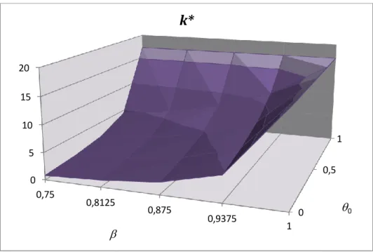
We illustrate the results with a small numerical example. Let = 1=3, A = 1 and = 0:05. The steady-state for capital and consumption is explored for values of 0 in the range 0 1 and values of in the range 0:75 1. Figure 3 shows how the amounts of capital and consumption vary with di¤erent values of the parameters that de…ne intertemporal impatience. The higher is 0, the larger are the equilibrium values of the two variables; the same occurs for a higher . The horizontal axis respects to , the depth axis represents di¤erent values of 0 and the vertical axis gives the values of each of the variables for the selected parameter values.
*** Fig. 3 ***
Although discounting is important in terms of the dynamics of the growth model, we conclude that it has a limited impact on the steady-state: parameter 1 does not have any in‡uence in long-run equilibrium, while a change on 0 disturbes the steady-state slightly by making the discount factor value to change in the same direction. A larger discount factor is synonymous of increased patience, which bene…ts the economy in terms of long-run accumulated capital and consumption levels.
5.2 Local Dynamics
In order to address stability properties, one needs to linearize the system in the vicinity of the steady-state point. Computation leads to
2 6 4 kt+1 k ct+1 c zt+1 c 3 7 5 = 2 6 6 4 1= 1 0 1 0 j 1 + 1 0(11 1) 1 1 0(1 1) 0 1 0 3 7 7 5 : 2 6 4 kt k ct c zt c 3 7 5 (13)
with j = 11 0 h 1 1 0(1 1) 1 i 1 1 (1 ) 1 0 1 (1 (1 ) ) 1 0 > 0.
Proposition 3 The system is saddle-path stable. There exists one stable dimension, in the three dimensional space of the model.
Proof. The existence of one stable dimension implies that one of the eigenvalues of the Jacobian matrix locates inside the unit circle, while the other two fall outside the unit circle. Let the eigenvalues be 1; 2; 3. We want to prove that j 1j < 1, j 2j > 1 and j 3j > 1.
We start by presenting trace, T r, determinant, Det, and sum of principal minors, M , of the Jacobian matrix; these are:
T r = 1+ 2+ 3 = 1= 1 0 + 1 + 1 0(11 1);
Det = 1 2 3= 1
( 1 0)2(1 1)
M = 1 2+ 1 3+ 2 3 = T r + Det + j 1
It is straightforward to observe that T r > 3, Det > 1 and M > 3. The constraint on the determinant implies that the eingenvalues are all positive or that 1 > 0; 2; 3 < 0. In this second scenario, the conditions involving the trace and the sum of principal minors imply 1 > 3 ( 2 + 3) and 1 < 32+2 33 ; these inequalities cannot be simultaneously satis…ed for the constraints on the values of the eigenvalues. Thus, the only feasible possibility is the one under which the eigenvalues are all positive: 1; 2; 3 > 0. If all the eigenvalues are larger than zero, then the constraints involving the trace and the determinant allow to perceive that full stability (all eigenvalues below one) is not a possible outcome. At least one eigenvalue must be larger than 1.
Next, we resort to Brooks (2004) to identify how many eigenvalues e¤ectively fall inside the unit circle. According to the mentioned author, an evaluation of the characteristic polynomial allows to state that: if condition
(1 + M ) < T r + Det < 1 + M
is met, there exists one real eigenvalue 1 of magnitude less than 1 and either: - a pair of complex conjugate eigenvalues 2; 3 = a ib, with ja ibj < 1; - two more real eigenvalues of magnitude less than 1; or
- a pair of real eigenvalues of magnitude greater than 1 and having the same sign. Since we have remarked that at least one of the eigenvalues is larger than 1, the only possibility that can hold from the three above is the last one. Thus, if the displayed double inequality is satis…ed, we con…rm that 0 < 1 < 1 and 2; 3> 1. It is straightforward to verify the validity of the condition since it is equivalent to
(T r + Det + j) < T r + Det < T r + Det + j
Therefore, we con…rm the existence of a single stable dimension, in the three dimen-sional space of the assumed system
The above result can be illustrated through a numerical example. Recover the bench-mark values for the exponential discounting bias case, i.e., = 0:97; 0 = 0:95; 1 = 23. For these, one computes the eigenvalues of the Jacobian matrix for various possibilities in terms of the values of 2 (0; 1) and 2 (0; 1), namely, we consider between 1=6 and 5=6 and between 0:025 and 0:125. The values that the eigenvalues possess for each combination of parameters are displayed in Figure 4. The …gure involves three panels, one for each eigenvalue. In the horizontal axis we have the values of , in the depth axis the value of and in the vertical axis the values assumed by each eigenvalue. Panel a respects to 1 and the other two to the eigenvalues that fall outside the unit circle, independently of the values of the parameters.
*** Fig. 4 ***
With saddle path stability, we have a result that is qualitatively similar to the one of the original Ramsey model with a constant discount rate. There is convergence towards the unique steady-state point, along a one-dimensional stable path; this trajectory is followed because the representative agent has the possibility of adapting its initial consumption level in order to place the system over the stable path, since consumption is a control variable. The expression of the stable trajectory can be presented in general terms. Proposition 4 Consider a point (k0; c0) in the vicinity of the steady-state (k ; c ). In the convergence from the …rst to the second point, contemporaneous values of consumption and capital evolve following the stable path
ct c = 1= 1 0 1 (kt k )
Proof. The saddle-path stable trajectory can be obtained by computing the eigenvec-tor associated to the eigenvalue inside the unit circle. Thus, we can solve the system
2 6 6 4 1= 1 0 1 1 0 j 1 + 1 0(11 1) 1 1 0(11 1) 0 1 1 3 7 7 5 2 6 4 p1 p2 p3 3 7 5 = 2 6 4 0 0 0 3 7 5
Letting p1= 1, the eigenvector might be written as
P = 2 6 4 1 1= 1 0 1 1=( 1 1 0) 1 3 7 5
The slope of the contemporaneous relation between consumption and capital is given by the ratio p2=p1, i.e., ct c = (p2=p1) (kt k ), which corresponds to the expression in the proposition
As in the original Ramsey model, the convergence relation between capital and con-sumption is of positive sign; thus, values of both variables are likely to simultaneously increase towards their long-term values. Note that this is a generic stable path expression that can be applied to speci…c forms of the discount function, namely the quasi-hyperbolic case and also the pure exponential discounting case. Observe, as well, that another stable trajectory emerges from the analysis: one can also relate consumption at t 1 to the capital stock at t. This convergence relation is also of positive sign.
Let us return to the numerical example. Take = 1=3 and = 0:05 and recover the remaining parameter values of the benchmark exponential discounting bias exercise. The eigenvalue inside the unit circle is, in this case, 1 = 0:944 14. The stable trajectory is, then, ct c = 5: 738 4 10 2(kt k ). For the assumed parameter values, in the conver-gence towards the steady-state, when the capital stock increases by one unit, consumption will increase 5: 738 4 10 2 units. This rate of convergence can be compared to the one of the quasi-hyperbolic discounting setting. Recall that hyperbolic discounting was discussed for b = 0:6; b = 0:99, with b = 1 and b = (1 0).
Continue to consider = 0:97; to be in the conditions of the QHD case, we must now take 0 = 0:67004 and 1 = 16: 771. For these parameter values, the lower than 1 eigenvalue comes 1 = 0:936 68 and the stable trajectory is now ct c = 7:342 1 10 2(kt k ). In the QHD case, the saddle path is steeper than in the EDB case. If we take EDB as a closer approximation to pure hyperbolic discounting, one possible error in using QHD consists in achieving a larger change in consumption as the capital stock evolves than the one that should, in fact, be obtained.
Next, we consider the constant discount rate case. This is the case for which 0 and 1 are zero. As 1 approaches zero, the eigenvalue lower than 1 approaches 0:917 99. Thus, the stable trajectory is ct c = 0:11294(kt k ). This case departs even more from the hyperbolic discounting case and thus the relation between k and c is even more steeper.
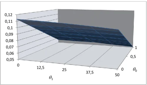
The above results point to the conclusion that the further we are from the exponential discounting case the less consumption will vary, in the convergence towards the steady-state, as the capital stock evolves. To emphasize this outcome, let us present the slope of the stable trajectory for di¤erent values of 0 and 1. Consider, again, = 1=3, = 0:05, = 0:97. Figure 5 takes 1 in the horizontal axis and 0 in the depth axis, in order to quantify the slope of the stable arm in the vertical axis. It is evident from the …gure that a larger bias relatively to exponential discounting (measured by higher values of 0 and 1) implies a smaller change in c relatively to k in the process of adjustment towards the steady-state.
6
Habit Persistence
In this section, we extend the discounting bias analysis to a setting where consumption choices are subject to habit persistence. This extension serves the purpose of showing that the adaptation of the standard intertemporal optimization model in order to include the discounting bias is ‡exible enough to approach other meaningful issues concerning the analysis of utility dynamics.
Habit persistence is modeled through the consideration of the following utility func-tion,2
u(ct; ct 1) = ln(ct bct 1); b 2 [0; 1) (14) According to (14), when b = 0, we have the conventional version of the model without habit persistence; a positive b indicates that utility is directly dependent on how much more the individual consumes today, relatively to consumption in the previous period. As it is obvious, the larger the value of b the stronger is the habit persistence e¤ect. Constraint ct> bct 1 must hold, in order to guarantee a feasible solution.
Consider the problem in section 4, relating utility maximization under the exponential discounting bias, subject to resource constraint (4). Now, the problem takes the form
V (at) = max c n u(ct; ct 1) + 1 0 h V (at+1) (1 1)u(ct+1; ct) io (15) Following the same procedure for the computation of …rst-order conditions as before, one arrives to the dynamic equation of consumption,
ct+1= bct+ 1 0(1 1)(1 + r) 2 1+r ct bct 1 1 1 0(ct 1 bct 2) (16) which is equivalent to t+1= b + 1 0(1 1)(1 + r) 2 1+r t b 1 1 0(1 b= t 1) 1 t (17)
Proposition 5 The optimal control problem of the representative household under expo-nential discounting bias and habit persistence has three steady-state points: = 1 0(1+
r) _ = 1 0(1 1) _ = b.
Proof. By taking := t+1= t, one transforms di¤erence equation (17) into `1( )3 (`2+ b`1) ( )2+ (`3+ b`2) b`3 = 0;
with `1:= 1= 1 0, `2 := 2 1 + r and `3:= 1 0(1 1)(1 + r):
2
See Heer and Maussner (2005) for a more general presentation of the utility function with habit persistence and corresponding analytical treatment.
The solutions of the equation are = `2 p`22 4`1`3
2`1 _ = b, which correspond to the
ones in the proposition
Comparing with the problem without habit persistence, we have now an additional solution, = b, but the other two remain exactly the same. Again, the representative agent chooses the path that opens the door for a possible positive steady-state growth rate of consumption, i.e., 1 = 1 0(1 + r) 1.
If we include the habit persistence feature in the growth model with capital accumula-tion, the result is that, once more, this extension does not interfere with the steady-state outcome and with the stability properties of the system. The steady-state continues to correspond, as before, to a saddle-path stable equilibrium. Under habit persistence, sys-tem (12), which characterized growth dynamics, takes now the form of a four-dimensional set of relations, 8 > > > > > > > < > > > > > > > : kt+1= Akt ct+ (1 )kt ct+1= bct+ 1 0(1 1)h1+ Ak (1 ) t i 2 1 + Akt(1 ) ct bzt 1 1 0 (zt bvt) zt+1= ct vt+1= zt (18)
In the steady-state, c := ct+1 = ct= zt= vt and k := kt+1= kt. The evaluation of (18) under the previous conditions leads to an exact same outcome as the one in proposition 2. Habit persistence does not change the unique equilibrium point towards which the economy converges in the long-run.
Stability could be addressed as in the case b = 0. We present the linearized system, in the steady-state vicinity, but we do not pursue a generic discussion on the signs of the eigenvalues. Instead, we just characterize stability resorting to a small example. The linearized system is:
2 6 6 6 6 4 kt+1 k ct+1 c zt+1 c vt+1 c 3 7 7 7 7 5= 2 6 6 6 6 4 1= 1 0 1 0 0 j(1 b) 1 + bj + b bj(1 + b) b bjb 0 1 0 0 0 0 1 0 3 7 7 7 7 5: 2 6 6 6 6 4 kt k ct c zt c vt c 3 7 7 7 7 5 (19)
where j is the same combination of parameters as in section 5 and bj = 1 0(11 1).
Reconsider the numerical example of the previous sections ( = 0:97; 0 = 0:95; 1 = 23; = 1=3, A = 1; = 0:05). For these values, independently of the degree of habit persistence (i.e., of the value of b), one …nds, for the Jacobian matrix in (19), a pair of eigenvalues inside the unit circle. Therefore, habit persistence does not change the stability result previously found: saddle-path stability holds, what implies that the representative agent will be able to control the consumption path in order to place the system on the stable arm, through which the economy converges towards the steady-state.
7
Conclusion
People do not evaluate future outcomes as if they were computers or calculators. Mea-suring the future value of some current event or the present value of some future event is many times an intuitive process in which individuals engage. In the same way there is evidence of an exponential growth bias, according to which individual agents tend to lin-earize the sequence of accumulated future outcomes, we can conceive a kind of exponential discounting bias, according to which we may explain the evidence that points to decreasing impatience and that is analytically translated in the concept of hyperbolic discounting.
The notion of exponential discounting bias is more general than the one commonly used by economists to characterize observed intertemporal preferences, i.e., the notion of quasi-hyperbolic discounting. This allows for a ‡exible analysis, where we can shape the trajectory of the discount factor in the way we …nd more reasonable in order to be as close as possible to what evidence reveals.
Furthermore, the new speci…cation has appealing features from an analytical tractabil-ity point of view: because the bias originates on a misperception about how to evaluate the future that does not introduce any kind of sophistication on individual behavior, i.e., any kind of ability to understand that the perception of the future will change as time evolves, the optimization model can be approached similarly to what is done in the exponential discounting case.
When assessing the dynamics of an intertemporal representative consumer growth model in discrete time, the exponential discounting bias assumption has allowed to con-struct a three dimensional dynamic system, from which it is straightforward to analyze steady-state properties and transitional dynamics. The analysis makes it possible to pro-ceed with a thorough characterization of how di¤erent intertemporal preferences may shape the optimal relation between capital accumulation and consumption.
The exponential discounting bias concept is adaptable to other features of the bench-mark utility analysis. Speci…cally, in this paper, one has explored the implications of introducing habit persistence into the utility function; the conclusion is that steady-state and stability results remain basically the same when the new assumption is taken into consideration.
References
[1] Akerlof, G.A. (1991). ’Procrastination and Obedience.’American Economic Review, vol. 81, pp. 1-19.
[2] Almenberg, J. and C. Gerdes (2011). ’Exponential Growth Bias and Financial Liter-acy.’IZA discussion paper no 5814.
[3] Barro, R.J. (1999). ’Ramsey Meets Laibson in the Neoclassical Growth Model.’Quar-terly Journal of Economics, vol. 114, pp. 1125-1152.
[4] Benhabib, J.; A. Bisin and A. Schotter (2010). ’Present-Bias, Quasi-Hyperbolic Dis-counting, and Fixed Costs.’Games and Economic Behavior, vol. 69, pp. 205-223. [5] Bialaszek, W. and P. Ostaszewski (2012). ’Discounting of Sequences of Delayed
Re-wards of Di¤erent Amounts.’Behavioural Processes, vol. 89, pp. 39-43.
[6] Bleichrodt, H.; K.I.M. Rohde and P.P. Wakker (2009). ’Non-Hyperbolic Time Incon-sistency.’Games and Economic Behavior, vol. 66, pp. 27-38.
[7] Brooks, B.P. (2004). "Linear Stability Conditions for a First-Order Three-Dimensional Discrete Dynamic." Applied Mathematics Letters, vol. 17, pp. 463-466. [8] Coury, T. and C. Dave (2010). ”Hyperbolic’ Discounting: a Recursive Formulation
and an Application to Economic Growth.’Economics Letters, vol. 109, pp. 193-196. [9] Dasgupta, P. (2008). ’Discounting Climate Change.’Journal of Risk and Uncertainty,
vol. 37, pp. 141-169.
[10] Dimitri, N. (2005). ’Hyperbolic Discounting can Represent Consistent Preferences.’ University of Siena, Department of Economics working paper no 466.
[11] Drouhin, N. (2009). ’Hyperbolic Discounting may be Time Consistent.’ Economics Bulletin, vol. 29, pp. 2549-2555.
[12] Farmer, J.D. and J. Geanakoplos (2009). ’Hyperbolic Discounting is Rational: Valuing the Far Future with Uncertain Discount Rates’Cowles Foundation Discussion Papers no 1719.
[13] Gollier, C. (2010). ’Expected Net Present Value, Expected Net Future Value, and the Rmasey Rule.’ Journal of Environmental Economics and Management, vol. 59, pp. 142-148.
[14] Gollier, C. and M. Weitzman (2010). ’How Should the Distant Future be Discounted when Discount Rates are Uncertain?’ Economics Letters, vol. 107, pp. 350-353. [15] Gong, L.; W. Smith and H. Zou (2007). ’Consumption and Risk with Hyperbolic
Discounting.’Economics Letters, vol. 96, pp. 153-160.
[16] Graham, L. and D.J. Snower (2007). ’Hyperbolic Discounting and the Phillips Curve.’ Kiel working paper collection no 2.
[17] Groom, B., C. Hepburn, P. Koundori, and D. Pearce (2005), "Declining Discount Rates: The Long and the Short of it", Environmental and Resource Economics, vol. 32, pp. 445-493.
[18] Heer, B. e A. Maussner (2005). Dynamic General Equilibrium Modelling – Computa-tional Methods and Applications. Berlin: Springer.
[19] Hepburn, C.; S. Duncan and A. Papachristodoulou (2010). ’Behavioural Economics, Hyperbolic Discounting and Environmental Policy.’Environmental and Resource Eco-nomics, vol. 46, pp. 189-206.
[20] Japelli, T. (2010). ’Economic Literacy: an International Comparison.’ Economic Journal, vol. 120, pp. F429-F451.
[21] Kahneman, D. and A. Tversky (1979). ’Prospect Theory: an Analysis of Decision under Risk.’Econometrica, vol. 47, pp. 263-292.
[22] Laibson, D. (1997). ’Golden Eggs and Hyperbolic Discounting.’Quarterly Journal of Economics, vol. 112, pp. 443-478.
[23] Laibson, D. (1998). ’Life-Cycle Consumption and Hyperbolic Discount Functions.’ European Economic Review, vol. 42, pp. 861-871.
[24] Loewenstein, G. and D. Prelec (1992). ’Anomalies in Intertemporal Choice: Evidence and an Interpretation.’Quarterly Journal of Economics, vol. 57, pp. 573-598.
[25] Lusardi, A. (2008). ’Financial Literacy: an Essential Tool for Informed Consumer Choice?’ NBER working paper no 14084.
[26] Noor, J. (2011). ’Intertemporal Choice and the Magnitude E¤ect.’Games and Eco-nomic Behavior, vol. 72, pp. 255-270.
[27] O’Donoghue, T. and M. Rabin (1999). ’Doing It Now or Later.’American Economic Review, vol. 89, pp. 103-124.
[28] Phelps, E.S. and R.A. Pollak (1968). ’On Second-Best National Saving and Game-Equilibrium Growth.’Review of Economic Studies, vol. 35, pp. 185-199.
[29] Pollak, R.A. (1968). ’Consistent Planning.’Review of Economic Studies, vol. 35, pp. 201-208.
[30] Prelec, D. (2004). ’Decreasing Impatience: a Criterion for non-Stationary Time Pref-erence and ’Hyperbolic’Discounting.’Scandinavian Journal of Economics, vol. 106, pp. 511-532.
[31] Rasmussen, E.B. (2008). ’Some Common Confusions about Hyperbolic Discounting.’ Indiana University, Kelley School of Business, working paper of the department of Business Economics and Public Policy no 2008-11.
[32] Rubinstein, A. (2003). ’Economics and Psychology? The Case of Hyperbolic Dis-counting.’International Economic Review, vol. 44, pp. 1207-1216.
[33] Stango, V. and J. Zinman (2009). ’Exponential Growth Bias and Household Finance.’ Journal of Finance, vol. 64, pp. 2807-2849.
[34] Strotz, R.H. (1956). ’Myopia and Inconsistency in Dynamic Utility Maximization.’ Review of Economic Studies, vol. 23, pp. 165-180.
[35] Walde, K. (2011). Applied Intertemporal Optimization. Mainz, Germany: Mainz Uni-versity Gutenberg Press.
[36] Xia, B. (2011). ’A Simple Explanation of Some Key Time Preference Anomalies.’ Canadian Journal of Economics, vol. 44, pp. 695-708.
1
Fig.1 – Discount factors for hyperbolic discounting, quasi-hyperbolic discounting and exponential discounting bias.
Fig.2 – Comparison between hyperbolic discounting and the two approximations (quasi-hyperbolic discounting and exponential
discounting bias). 0,3 0,4 0,5 0,6 0,7 0,8 0,9 1 0 2 4 6 8 10 12 14 16 18 20 22 24 26 28 30 32 34 36 38 40 42 44 46 48 HD QHD EDB time Discount factor 0 0,05 0,1 0,15 0,2 0,25 0 3 6 9 12 15 18 21 24 27 30 33 36 39 42 45 48 EDB-HD QHD-HD time Distance to hyperbolic discounting
2
Panel a – Capital stock steady-state value.
Panel b – Consumption steady-state value.
Fig. 3- Steady-state values of capital and consumption for different values of parameters β and θ0. 0 0,5 1 0 5 10 15 20 0,75 0,8125 0,875 0,9375 1
k*
0 0 0,5 1 0 0,5 1 1,5 2 0,75 0,8125 0,875 0,9375 1c*
0 3 Panel a – λ1
Panel b – λ2
Panel c – λ3
Fig.4 – Eigenvalues for different values of parameters η and δ (exponential discounting bias case).
1/6 1/2 5/6 0,6 0,8 1 1,2 0,025 0,05 0,075 0,1 0,125 1/6 1/2 5/6 0,8 1 1,2 1,4 0,025 0,05 0,075 0,1 0,125 1/6 1/2 5/6 1,6 1,8 2 2,2 0,025 0,05 0,075 0,1 0,125
4
Fig. 5- Slope of the stable trajectory for different values of parameters θ0
and θ1. 0 0,5 1 0,05 0,06 0,07 0,08 0,09 0,1 0,11 0,12 0 12,5 25 37,5 50 0 1