... : .::::::~: .
Praia de Botafogo, nO 190/10° andar - Rio de Janeiro - 22253-900
Seminários de Pesquisa Econômica I (2
aparte)
IIWELFARE AND FISCAL
POLICY WITH PUBLIC GOODS
AND INFRASTRUC'IIURE
11
\marf.
Pedro Cavalcanti Ferreira
EPGE/FGV
Coordenação: Prof. Pedro Cavalcanti Ferreira Tel: 536-9353
•
Welfare and Fiscal Policy with Public Goods and
Infrastructure
Pedro C. Ferreira Graduate School ofEconomics
Getulio Vargas Foundation Praia de Botafogo, 190 Rio de Janeiro, RJ, 22253-900
Brazil
We construct and simulate a model to study the welfare and macroeconomic impact of govemment actions when its productive role is taken into account. The trade-o:ff between public investment and public consumption is also investigated, since public consumption is introduced as a public good that directly affects individuals' well-being. Our results replicate econometric evidence showing that part of the observed slowdown of V.S. productivity growth can be explained by the reduction of investment in infrastructure, which also implied a sizable welfare loss to the population. Depending on the methodology used we found a welfare cost ranging from 4.2% to 1.16% of GNP. The impact of fiscal policy can be qualitative and quantitative distinct depending on whether we assume a higher or sma1ler output-elasticity to infrastructure. Ifit is high enough, increases in tax rates may stimulate accumulation and production, which is the opposite prediction of standard neoclassical models.
JEL Codes:
Keywords: Fiscal Policy, Welfare, Infrastructure, Labor Productivity.
..
Acknowledgments: We gratefully acknowledge the comments of Gary Hansen, Lee Ohanian, João Victor Issler and seminars and conference participants at Vniversity of Pennsylvania, PVC-Rio, Getulio Vargas Foundation and the SBE conference. We also thank Alessandra Gouvêa for the excellent research assistance and CNPq for the financial support.
•
1 Introduction
In the last few years a number of empirical studies, e.g. Aschauer(1989), Munnell(1990) and Nadiri and Mamuneas(l992), have investigated the productive impact of public infrastructure. These studies use different econometric techniques and data samples to estimate the output and the productivity elasticity to public capital. Overall, although the magnitudes found vary considerably, the estimates tend to confirm the hypothesis of a supply-side role for infrastructure capital 1. If that is the case, govemment expenditures cannot be thought of as a unique category, and the govemment choice of how much to spend on infrastructure and other expenses bears important welfare implications on equilibrium models.
In this artic1e we construct and simulate a model, c10se to the real business cyc1e tradition, to study the welfare and macroeconomic impact of govemment actions when its productive role is taken into account. Moreover, the trade-off between public investment and public consumption is investigated, since public consumption is introduced as a public good that directly affects individuais' well-being through the utility function.
The model will be used to answer some key questions concerning fiscal policy and welfare. With respect to fiscal policy we are most1y interested in investigating (through simulations) how different compositions of public expenses and taxes affect the behavior of the economy and private agents' decisions2. Regarding welfare, we want to study the impact of those altemative policies, and especially of changes in the public investment share, on agents' utility. Given the way the model is constructed, one extra dollar of public investment means one dollar less for public consumption, which direct1y reduces utility. The final effect, however, is unc1ear: public investment will boost private output and consequent1y private consumption and utility.
We initially compare the long-run properties ofthose altemative policies and later we assess the transition path of the economy after a policy change. In this process we will also compare the behavior of the economy assuming different intensities of output response to public investment, using altemative estimations from Ferreira(1993) and Aschauer(l989).
ITwo exceptions are Holtz-Eakin(1992) and Hulten and Swchartz(1992) who could find no evidence of ~ublic capital affecting productivity.
Part of our policy experiments in this section are similar to those in Baxter and King(1993). However, they do not distinguish between capital and labor income taxation and they have lump-sum transfers rather than
The motivation is that the evidences from these articles are very contrasting in magnitude: in the first paper the estimated elasticity is almost four times smaller than in the second.
Our results conceming policy will replicate econometric evidence, e.g. Morrison and Schwartz(1992), showing that part ofthe observed slowdown ofproductivity growth in the seventies and eighties can be explained by the reduction of investments in infrastructure. In
this particular experiment, for instance, tax rates are kept constant while the share of • investment out oftotal public expenditure, following recent U.S. experien~e, decreases. The
policy simulations will also show that the impact of fiscal policy can be qualitative distinct depending on whether we assume a higher or smaller output elasticity to infrastructure. If it is high enough, increases in tax rates may stimulate accumuIation and production, which is the opposite prediction of standard neoclassical models.
When investigating welfare, we will see that there is much to be gained only by shifting public expenses from consumption to investment, even when public consumption directly affects utility or when output eIasticity to public infrastructure capital is relatively small. The reason is that the positive impact on output and private consumption caused by the increase in public investment, in general, dominates the negative impact on welfare of the smaller share of public consumption. Consequently, according to our simuIations, the observed sIowdown of public investment in the U.S. implied a sizable welfare Ioss to the population. Depending on the methodoIogy used, we found a welfare cost ranging from 4.2% to 1.16% ofGNP.
Another important implication of the welfare simulations is that govemments can be tempted to unexpectedly increase consumption because of short-run welfare gains. Govemments are short-lived and although the Iong-run outcome at present value may represent a welfare Ioss (if the investment share decreases), the political benefits of 4 or 8 years of increased consumption couId well decide in favor of this kind of policy even if
consumption will eventualIy falI in the Iong-run .
The paper is organized as follows: in the next section the model is presented and in the following we discuss the soIution method and the calibration procedures; section four reports the outcome ofthe fiscal policy experiment for the steady state: section 5.a discusses steady-state weIfare and section 5. b presents both the welfare and fiscal policy effects outside the steady state. Finally, in section 6 some concIuding remarks are made.
•
2 TheModel
Consider an econorny where individuals live forever and obtain utility frorn leisure, private consurnption and govemment consurnption. Govemment consurnption is basica1ly a public good which does not suffer frorn congestiono Preferences are given by:
CIO
(1.1)
:LP
{log(cPt+
,uCg,)
+
Alog/,} O<P<It=O
In the above expression cp is private consurnption, Cg public consurnption and I is leisure. The parameter J..L can assume any value, but if it is one the consurner equally values
public and private consurnption. If J..L is zero the consurner does not care for public goods.
Households maximize (1.1) subject to a sequence ofbudget constraints:
Households divide their purchases between consurnption goods and investrnent goods Ot). The funds available for these purchases include after-tax capital incorne, where rt
is the rental rate of capital, kt the stock of capital owned by the household and '" is the tax rate on capital incorne and after-tax labor incorne, (l-tb)wtht where Wt is the wage rate, ht hours worked and th is the tax rate on labor incorne. Total hours are normalized to one so that:
(1.3) ht
+
It = 1The law ofrnotion of( private) capital is:
In this economy the production function has constant retums to scale to private inputs and is subject to technology shocks. It also includes public capital (Kgt) as a separate argument. This assumption follows Barro(1990), Barro and Sala-i-Martin(1993) and Aschauer(1989). It implies that public and private capital are not perfect substitutes and that public capital, e.g. infrastructure, is essential to private production. The technology is thus given by:
(1.5)
J;
= exp(Zt) .Kg/ KtB n<,l-B)Capital letters are used to represent per capita variables taken as given by the household, while small letters represent individual specific variables chosen by the household. In equilibrium those variables wiIl be the same. The exogenous technology shock follows a law of motion given by
(1.6) Zt+1 = PZt + &t+1, O ~ P ~ 1
In the above expression Et is an iid random variable with mean zero and variance O"E2.
It is also assumed that all agents know Zt in the beginning of period t.
Govemment raises taxes on capital and labor incomes in order to finance its expenditures in consumption and investment. We rule out govemment bonds so that the budget constraint of the public sector is in equilibrium every period:
Tax rates are fixed in this economy and we also assume that govemment follows a fixed and known rule to divide its expenditures between investment and consumption:
(l.8) Cgt = (l-a) Gt O~a.~l
•
In this set-up a fiscal policy is represented by the two tax rates and alpha, the
proportion of total govemment expenditures allocated to investment. The public capital law of motion is given by
The problem ofthe finns is to maximize profits, 1r = ft - WtHt - rtKt, every period.
From the first order conditions of this problem we obtain the following functions for the rental rate of capital and wage rate:
(1.12)
The household's dynamic problem can be expressed as:
V(kt,Kt,Kgt,ztJ = max (U(cPt+pCgt,l-htJ +
pE
V(kt+1,Kt+1,Kgt+1,Zt+1)} subject to Ct +it
= (1-w ht + (1-TJr) kt Zt+1 = PZt + &t+1, kt+1 =it
+ (1-8) kt , Kt+1 = It + (1-8) Kt, Kgt + 1 = Igt + (1-ogJ
Kgt Igt =aGt
In the above problem V( ) is the equilibrium maximized present value of the utility flow of a household who enters the period t with kt and knows that the aggregate state is described by Kt, Kgt, Zt. In solving his problem the representative householder takes into account that the wage rate and the rental rate are given functions of the aggregate state. The households also take the evolution of Kt and Kgt as given. In addition, H and I are given functions of Kt, Kgt, Zt.
A recursive competitive equilibrium is a set of household decision rules,
i( kt, Kt, Kgt, z(}, h( kt, Kt, Kgt, z(} and c( kt, Kt, Kgt, z(}, a set ofper capita decision rules
I ( Kt, Kgt, ztJ and H (Kt, Kgt, ztJ, a set of pricing and public expenditure functions, w( Kt, Kgt, ztJ, r( Kt, Kgt, z() and G( Kt, Kgt, ztJ and a value function V( kt, Kt, Kgt, z(} such that:
(i) households solve problem (1.12) taking as given I, H and G.
(U) I( Kt, Kgt, z(} = i(Kt, Kt, Kgt, ztJ and H( Kt, Kgt, ztJ = h(Kt, Kt, Kgt, z(}
(iU) The market for final goods c1ear each period
C(kt, Kt, Kgt, ztJ + I(kt, Kt, Kgt, z(} + G( Kt, Kgt, z(} = Y( Kt, Kgt, z(}
3 Solution Method and Calibration Procedure
We solve the model using numerical methods. For the experiments of section four we used the first order conditions to find steady-state expressions for private capital, hours worked and public capital in terms of technology, preferences and fiscal policy parameters. We used these expressions to perform policy experiments.
In section five we solve the model using numerical methods due to Kydland and Prescott(l982). However, given that the paper deals with a distortionary economy we cannot invoke the second welfare theorem to solve a planning problem. For this reason, we follow more c10sely the recursive method described in Hansen and Prescott(1995) for this c1ass of economies.
We start eliminating private consumption in the utility function using· household budget constraint and thefunctions w() and r( ). We next find first order conditions for the household problem which are nonlinear. In order to obtain an analytical solution for this problem we form a linear quadratic approximation around the steady state. We first solve for
..
the steady state by substituting for public consumption a( tk r( ) K + th w()H) and then compute the linear-quadratic approximation. The final step is to solve this dynamic programming problem iterating on the now quadratic Bellman's equation imposing at each step that equilibrium condition (li) holds. After convergence we obtain equilibrium expressions for the aggregate labor and investment decision roles in terms of Zt , Kgt anti Kt, as kt
=
Kt in equilibrium.We will use these expreSSlOns, along with the laws of motion of capital and
technology shock, the production function and expression (1.7) of govemment
expenditures, to simulate the economy for different fiscal policies. However, in order to use this methodology we had fust to make the (strong) assumption that public investment rather than public capital, is the argument ofthe production function (or, equivalent1y, we have to assume full depreciation of public capital). Once we place Igt in the production function, we have to transform variables by applying logarithms. This transformation is necessary because after substituting for Wt, rt and ht in the utility function there is still one nonlinear expression to be eliminated, which is
Kgt+ 1 = Igt + (l -8) Kgt= (l -a)( Tk rt Kt + Th WtHt) + (l -8) Kgt =
(l-a) (Tk8 + Th{l-8)) exp(zt}.Kgt;Kt8H/ 1-8)
+
(1-8) KgtWe cannot plug this expression into the utility function and the methodology cannot be used for nonlinear expressions. Our solution was to assume that Kgt+ 1 = Igt and to
apply logs to obtain
-In the above expression X represents the logarithm of the variable X. We next applied logs to alI (steady-state) variables and we plugged the investment equation ( it
=
kt+ 1 - (l-õ)kt) into the utility function in order to be Ieft only with (log) linear expressions outside it. The functional values are not affected because inside the utility function we used the exponential of X, whenever the variable "X" showed up.The parameter values used in both groups of simulations (steady-state and transition path simulations) follow closely the values used in most of the recent RBC literature and are
..
intended to match those observed in the US economy. The labor share is assigned to be 70%, the average over the 48-85 period, and a magnitude used, for instance, by Greenwood, Hercowitz and Krussel(1992), as well as by Hansen and Prescott(1993). The depreciation rate for public and private capital is set at 0.02 per quarter, smaller than in Prescott(1986), but in line with Christiano(l988), Hansen and Prescott(1993) and Greenwood et alI. We used 0.99 for the discount rate, a value used by almost every paper in the literature. It
implies an interest rate of 6.5% a year. The parameters p and 08 are set to be 0.95 and
0.00716, which we estimated for a production function with public 'expenditures as a separated argument. As in Cooley and Hansen(1992), Ais equal to 2 in the simulations. This value implies that the households alIo cate 2/3 of their time to non-market activities.
We arbitrarily set ~ to be equal to one, implying that consumers give the same weight to public and private consumption. We did that for three reasons. First, we do not know of any estimates of this parameter in the literature, so that any value would end up being arbitrary. Second, for the policy experiments we ran, changes in this parameter did not affect qualitatively the results but only their magnitude. FinalIy, smalIer ~ values strengthen the argument for investments with regard to public consumption. If ~ is zero, the altemative to investments is "waste", which would make this problem trivial. Giving equal weight to public consumption and investment in consumer welfare, we emphasized the trade-off between the two types of public expenditure.
The remaining parameters, with the exception of q" are alI policy parameters and will
be changed according to the policy experiment performed. The base parameters, which will
be calIed standard economy, are the following. Alpha is set to be 0.12 since this is the average of infrastructure and equipment expenditures out of total govemment expenses for the 1972-1988 period. Labor and capital tax rates follow Cooley and Hansen(1992): tk equal to 0.5 and th equal to 0.23.
FinalIy we set
q,
equal to 0.09, which is the value estimated in Ferreira(1993) for US quarterly data. This value is well below previous estimates, particularly estimations in Aschauer(1989), so that we also usedq,
equal to 0.35 to compare the response of the economy to policy changes with these two different elasticities .•
4 Long-Run Analysis
Changes in fiscal policy, and more specifically in the composition of public expenditures, have a significant influence on the steady-state path of this economy. Figure one displays steady-state leveIs of productivity as alpha, the proportion of investment in total public expenditures, increases and tax rates are kept constant.
Figure 1:
Steady-state Productivity LeveIs
(<I>
=0.09)
2.6 2.4 2.2 ..., 2.0 ~ o.. ..., ~ o 1.8 1.6 1.4
--
--~ ~----J~-'
V-/ '
V
/
v
I
I
1.2 0.0 0.1 0.2 0.3 0.4 0.5 0.6 0.7 0.8 0.9 1.0 AlphaSteady-state productivity increases continuously with a.. If this variable increases trom 0.11 to 0.12, the U.S. average trom 1972 to 1988, productivity will rise by 1.2 percent. Note also that most of the gains are obtained when investment goes trom zero to 20% of public expenditures. It increases fifty seven percent in this interval while increasing only thirty one percent when the proportion of investment goes trom twenty to ninety nine percent of the total. So fiscal policy, through public investment, can affect productivity leveIs, but at decreasing retums. An interesting implication of this fact is that, at least as a
policy to increase productivity, governrnents do not need to dedicate politica1ly unrealistic proportions of their budgets to investment since the returns rise more slowly as the investment share gets larger.
As we will see below in figure 2, increases in alpha also lead to increases in output. Moreover, the ratio of public investment to output also rises, as the latter grows less then the former. Hence, for the long run at least, this result matches the empírical findings of Aschauer(1989) and Morrison and Schwartz(1992), namely that change~ in the proportion of public investment to GNP induce changes in labor productivity in the same direction. These articles and the simulations presented here conclude that part of the slowdown of productivity growth observed in the U. S. in the last two decades might be explained by the fact that the ratio ofpublic investment to output felI from 14.3% in 1972 to 10.8% in 1988.
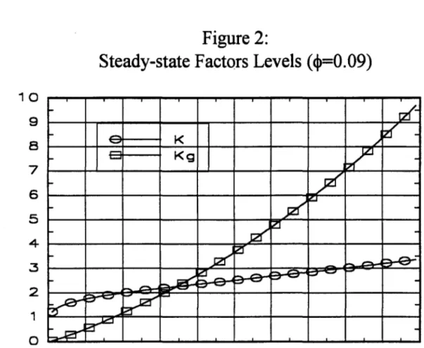
Figure 2 below plots the steady-state leveis of capital stock and governrnent investment against alpha leveis.
10 9 8 7 -+-' 6 :::::I o- 5 -+-' :::::I
o
4 3 2 1 OFigure 2:
Steady-state Factors Leveis (cp=O.09)
-
K-
... Kg ... ... ~....
~
~~
r-~ ~ 0.1 0.3J2I
JZf'
zr ~ r-0.5 Alphatzf
/zf
~
yJ'
;zI
~ íZI -~ -0.7 0.9Hours (not included in the above figure because of scale problems) increase with
a
because the return to labor increases with public investment. A greater number of hours worked leads to higher income and investment and therefore higher capital. The return to capital also increases with public investment so that there is an additional force pushing investment and capital stock to higher steady-state leveIs. However, a different behavior could be expected. Given G, the reduction of alpha causes a decrease in public consumption which leads to a decline in consumer's utility. This could induce an increase in private consumption to compensate for the loss of govemment consumption and, 'consequent1y, to a drop in private investment and capital stock. It turns out that this is never the case and the impact on private returns always dominates so that income, investment ( public and private), consumption, tax revenues and govemment expenditures grow with alpha, for any J..I. we use.
In the remaining part of this section we compare two economies similar in every aspect but the coefficient <1>, the output elasticity of public expenditures. Our motivation for this experiment is that the impact of tax changes on the steady-state path of the economy is high1y influenced by this elasticity. We take phi close to Aschauer's(l989) estimations, 0.35, as well as phi close to estimations from Ferreira(1993), 0.09. In the flrst case, public infrastructure is so productive that tax increases up to leveIs above or close to the American leveIs may in fact stimulate activity, accumulation and employment: the negative effect ofthe increased taxes on returns is smaller than the positive effect due to the investment they finance. Hence, the simulations qua1ify the findings in Aschauer, as they show that his estimations imply that ifthe govemment raises labor tax from 0.23 to 0.30, production will
rise, not falI. In this case the policy recommendation of the model would be to increase taxes during recessions and decrease them during booms.
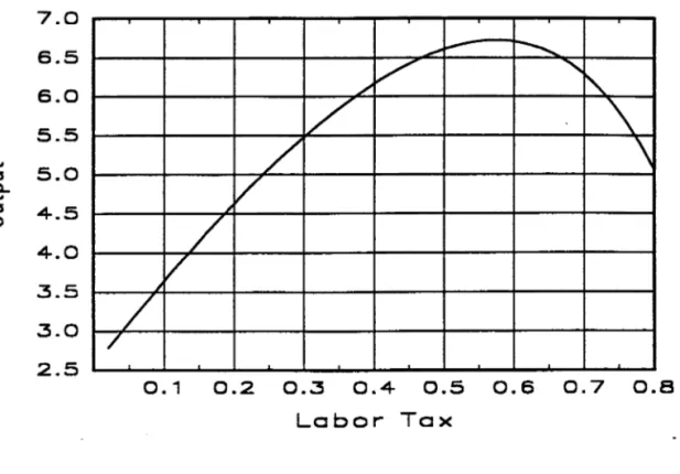
Figure 3 presents the steady-state leveIs of income for different labor tax rates for the "standard" economy (<I> = 0.09) for alpha equal to 0.12 ( the average value for the American economy), alpha equal to one half and equal to ninety percent. Figure four displays income leveIs for the "Aschauer" economy (<1>=0.35) when alpha is 0.12.
0.9 0.8 ~a-0.7 _G 0.6 -+-' ~ c... 0.5 -+-'
-~ O 0.4 0.3 0.2 lo- I-0.1Figure 3:
Steady-State Output LeveIs (Phi
=0.09)
A A A A ~
~
-'""""'-."
-
rts..~
l.~
-
...~
"'t .,. ~ rs. ~~
~~
e Alphc=O.12--~
~ El Alphc=O.50 é Alphc=O.90~
0.1 0.2 0.3 0.4 0.5 0.6 0.7 0.8 Labor TaxFor the standard economy any increase in the labor tax rate, when alpha is equal to 0.12, will reduce the output levei in the steady state. Tax rates as low as 2% are sufficient to induce a drop in output in the same way as in models without public capital in the production function. This is not the case for the "Aschauer" economy: Steady-state income starts to falI only when 'th is greater than 0.32. For values below this threshold, income leveI actually goes up with the labor tax rate. In this case, public investment is so productive that its impact on capital and income is strong enough to overcome the negative effect on retums due to higher taxes.
7.0 6.5 6.0 5.5 -'" 5.0 ::::s c... -'" ::::s 4.5 O 4.0 3.5 3.0 2.5
Figure 4:
Steady-State Income LeveIs
(<j)
=
0.35,
a
=
0.12)
/
-
-
...V
... ~ . // '
'\
/
\
/
/
/
/
0.1 0.2 0.3 0.4 0.5 0.6 0.7 0.8 Labor TaxFor ratios of public investment well above 0.12, the behavior of these economies is somewhat harmonized but only up to a certain extent. The two upper curves in figure 3 display the steady-state income leveIs in the standard economy when alpha is 0.5 and 0.9. In
the last case, steady-state income grows with th for rates below 0.32 and for alpha equal to 0.5 it remains barely constant for rates below 0.08 and then it falls. However, for the "Aschauer" economy in the case of ex
=
0.9 and ex=
0.5 income grows with th for rates up to 0.62 and 0.42, respectively. In other words, in an economy where output elasticity to public capital is around 0.35, labor tax-rate raises up to certain limits increase the income leveI in the steady state. For smaller elasticities ( cI>=
0.09 in the present case), this is onlythe case when the proportion of investment out of total public expenditures is considerable higher than the actual ratio for the USo economy.
Figure five below tries to clarify these relationships. It shows the steady-state leveIs of factors of production for the case where ha1f the expenditures goes to investment and phi is 0.35 (labor was excluded because its scale is toa small compared with the other factors).
180 160 140 120 100 80 60 40 20
o
Figure 5:
Steady-state Factor LeveIs
(</>
=
0.35,
a
=
0.12)
,.-/ ~
~
J;V
L./
-~
./;zf
-
I</
......
k G /~ -~ ~- -
-
-
-
-
-
-
-c: -~ 0.1 0.2 0.3 0.4 0.5 0.6 0.7 0.8 Labor TaxAs 'th increases, total tax collection and consequently public investment follow in the same direction. Everything else being the same, the retum to capital and labor would rise with public investment. However, the higher taxes reduce the retum to labor and dominate the investment effect so that hours worked decreases, in the steady state, with labor tax rates. Less hours would lead to lower income and investment and therefore to lower capital stock. For tax rates below some threshold (0.52 in this case), this force is weaker than the direct effect on capital retum due to higher public investment, so that steady-state capital stock increases initialIy. With capital and public investment increasing with labor tax, income also rises, although hours worked are smalIer. In the economy where cI> is 0.09, the direct effect on retums is never strong enough (unless we assume unreasonable high alphas) to compensate for the drop in hours, so that both capital and income steady-state leveIs falI with the labor-tax rate. The disincentive to work resulting from higher taxes exceeds the gain in retums induced by higher investments.
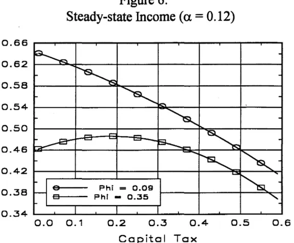
The behavior of these economies is even more distant when we look at the income .. responses to variations in capital tax rates displayed in the figure below.
Figure 6:
Steady-state Income (u
=0.12)
0.66 0.62 0.58 0.54 -+-' ~ c... 0.50 -+-' ~o
0.46 0.42 0.38~
-r~
,
~~
-=~
~-
-~-
~
~
...~'
o Phi=
0.09-
e Phi - 0.35"
0.34 I 0.0 0.1 0.2 0.3 0.4 0.5 0.6 Capital TaxFor the economy with the lower elasticity, steady-state income always falls with increases in 'tlc, no matter what parameter value of alpha is used in the simulations ( in the figure above it is 0.12). For the economy with <I>
=
0.35, there will always exist an interval oftax rates, for almost any alpha, where the steady-state income ( and capital stock) will be larger with higher capital tax rates. When alpha equals 0.12, the V.S. average, increases in
'tlc up to 0.221ead to rises in the steady-state income. In this case, as for the case oflabor tax increases, govemment investment is so productive that its effect on capital retums is stronger than the tax effect. For the case when phi is only 0.09, the tax effect always dominates, so that higher capital taxes always lead to decreases in the long-run leveI of mcome.
In summary: increases in the proportion of investment out of total public expenses lead to higher steady-state leveIs of capital, hours, income, labor productivity and attained utility. If the actual elasticity of output to public investment is closer to 0.35 then increases in both labor and capital tax rates lead, up to certain point, to increases insteady-state capital and income, so that higher taxes could actually stimulate the economy. However, if
that elasticity is closer to 0.09, higher taxes will always reduce the steady-state equilibrium leveIs of factors of production and output.
5 Welfare Comparisons
In this section we present two altemative estimates of the welfare costs of fiscal policies, while assuming different compositions of govemment expenditure and dilferent tax rates. Instead of comparing those alIocations with a Pareto optimal allocation for this economy, we compare welfare variations between two alternative policies'. BasicalIy we try to address the following question: what is the welfare loss ( or gain) for society of going from one given fiscal policy to another? Except for the fiscal policy parameters (
a,
'th and'tk), alI the parameters are the same as in the standard economy from the previous section, with alpha equal to 0.09.
5.a Steady-state Welfare
The fust welfare measure compares steady states and is due to Cooley and Hansen(1989). It is based on the change in total consumption ( private plus public) required to keep the consumer as well-off under the new policy as under the original one. The measure ofwelfare loss ( or gain) associated with the new policy is obtained by solving for x
in the following equation
(5. 1) U = ln( C· (1 + x))
+
A ln( 1- H·)In the above expression U is steady-state utility under the original policy, C* and H* are the total consumption and hours worked associated with the new policy. Total consumption is given by CPt + pCgt, IJ. being equal to one. Welfare changes will be expressed either as a percent of steady-state consumption (/lCI C) or as a percent of steady-state output (/l C/Y ) where /lC (= C* . x) is the total change in consumption required to restore an individual to the previous utility leveI.
For the steady-state welfare changes four dilferent groups of experiments are performed and displayed in table 1 below.
Table 1:
Steady-state Welfare
Simulation Original Policy NewPolicy áC/C áC/Y
a. tk th a. tk th One 0.50 0.50 0.23 0.88 0.50 0.23 12.26 9.12 One.b 0.85 0.50 0.23 0.90 0.50 0.23 5.0 4.2 Two 0.88 0.50 0.23 0.91 0.45 0.23 0.24 0.21 Three 0.88 0.50 0.23 0.76 0.45 0.23 -3.34 -2.97 Four 0.88 0.40 0.24 0.88 0.50 0.23 6.26 5.32 Four.b 0.88 0.50 0.23 0.88 0.45 0.23 -3.31 -2.80
The first simulation assumes a hypothetical economy with half of public expenditures going to investments, 'tk equal to 0.5 and th equal to 0.23. The welfare cost are considerable when alpha moves down to the U.S. average, which is 0.12, while keeping the tax rates constant. It is 12.26 when measured as a proportion of steady-state consumption ( áC/C) and 9.12 when measured as a proportion of steady-state output, still a significant value. From the previous section it is easy to understand the reasons for this fact. As the share of public investment out of total expenses drops, private investment, capital stock, hours worked and, consequently, output and consumption falI. With a smalIer steady-state output, tax collection also drops, so that not only private consumption but also total consumption steady-state leveIs end up being smalIer, despite the fact that the share of public consumption went up.
Even when values c10ser to the American experience are used, the welfare costs are substantial. From the beginning of the seventies to the end of the eighties expenditures in structures and equipment ofthe general govemment went from 14.3 % to 10.8% ofpublic expenses. In this case, the welfare costs of changing alpha from 0.15 to 0.1 ( simulation l.b) is 4.2 percent of GNP or 5 percent of consumption, when measured as áC/Y or áC/C, respectively. In other words, the slowdown of public investment in the seventies and eighties implied a sizable long run welfare loss to the population. At current leveIs, 4.2 percent of V.S. GNP amounts to approximately VS$ 250 billion, which is almost one thousand dollars per capita or the whole of Argentina's GNP.
The above results may be the most important lesson in this whole section: there is much to be gained by simply reallocating public expenses, without changing the tax structure, from non-productive consumption to investment in infrastructure and equipment. This is true even when it is taken into account that public consumption may affect individuals' well being.
Next, two stylized policy experiments are analyzed. In the first one ( simulation 2), the capital tax rate is reduced from the base value and, at the same time, t,he share of public consumption is increased. We can think of simulation 2 as a stylized conservative policy: capital-tax reduction and more expenditures on public goods such as defense, police and justice. The parameter 'tk goes from 0.5 to 0.45 while alpha falls from 0.12 to 0.09, which is slightly below where it stood in 1989. In this case the gains from the smaller taxes are canceled by the smaller investment share. There is a small welfare loss of 0.21 when measured as a proportion of output or 0.24 as a proportion of consumption. As a matter of fact, 'tk has to fall below 0.44 for there to be any welfare gains if the investment share of public expenditures drops to 0.09.
When keeping the share of investment constant at the base value, the gains from the reduction ofthe capital tax rate from 0.5 to 0.45 ( simulation 4.b) are considerable: 3.3% of steady-state consumption or 2.8% of steady-state output. As in standard real business cycle models, tax reduction is welfare improving, the difference in the present case being that there is a limit for tax reductions. Beyond this limit, welfare falls because the excessive decline in public investment, induced by lower taxes, negatively affects output and consumption. For instance, ifthe base policy is modified to one with a zero capital tax rate and labor tax close to zero, ( there is no equilibrium with both tax rates being exactly zero) the welfare cost as a percent change ofoutput is 321.4 !
The other stylized policy ( simulation 3) can be thought of as a stylized "liberal policy": relatively more investment in infrastructure and higher taxes. The liberal-style policy we simulate consists ofan increase of 10 percent in the capital-tax rate (from 0.50 to 0.55) and a twice-as-Iarge public-investment share (from 12% to 24%). The final result was a welfare gain of2.97 when measured by.1C IY and 3.44 when measured by.1C /C. As in the previous policy, there are two forces canceling each other out and part ofthe gains from the higher investment share is lost because of the increased taxes. If alpha alone changed, the welfare gains as a proportion of GNP would jump to 6.2%, more than twice the gains from the liberal-styled policy.
The last experirnent follows more directly the lines of Cooley and Hansen(1989) as we modified the mix of tax rates while keeping tax revenue, and alpha, constant. We start with a policy which has 'tk
=
0.4 and th=
0.24, and change it to the standard values, 'tk=
0.5 and th=
0.23. The welfare cost ofthis policy is 6.29 percent of steady-state consumption and 5.32 percent of steady-state output. The effect of the higher capital tax necessary to keep revenues constant in the face of smaller labor tax is strong enough to depress investment and income, and consequent1y private consumption, although public consumption remained the same. This is the expected outcome of capital tax increases in standard Neoclassical models.To sum up the steady-state experirnents, the simulations indicate that the reduction of public investment vis-à-vis public consumption observed in the American economy in the last two decades brought about a sizable welfare loss. Furthermore, policy proposals of increased investment financed by higher taxes ( the "liberal-style" experirnent) or reduced capital taxation accompanied by smaller investments (the "conservative-style" policy) need precise fine-tuning in order to prevent the gains from the change of one policy instrument from being lost with the modification of some other instrumento
The question we should ask whether those results still hold when we work outside the steady state and take transition paths into account. We answer this question in the next subsection.
S.b Welfare Changes and Transition Paths
The second welfare measure takes into account the transition from one policy to the other. Using methods due to Cooley and Hansen(1992), we construct for this model economy the transition between two steady states after a change in fiscal regime. We obtain
K, Kg and H for the entire path and with them we construct Cp, Gg and C. The welfare cost is calculated solving an equation like (5.1) for all the transition periods where C* and H* are substituted for the total consumption and hours for the period in questiono The welfare measure we use is the present value ofxCt over all periods of simulation as a percentage of the present value ofincome. Note that "x" above, as in the previous case, is the proportional change in total consumption required to keep consumers as well-off in the newpolicy as in the original one.
In the present method we first use a nonlinear equation solver to find the equilibrium capital leveI, hours worked and public investment in the transition path. The initial conditions are the steady-state values ofthe original policy. At every period we solve for the first order conditions and law of motion of public investment (given by equations 1.7 and
1.8):
(5.2) Ct+J - Ct
P
(rt (1-'t7J
+ (1-8)) = O(5.3) Wt (1--r;,) (1-HrJ - A Ct = O
(5.4) Kgt+J = (1-a)( TJcrtKt + 'rh WtHt )
To solve the above system, we first substitute the expressions for w, r, cp and Cg in order to obtain a system in terms on1y of K., H and Kg. The fiscal parameters are those for the new policy. This procedure is used from time zero to a given period T when the economy is close enough to the new steady state. From this period on the equilibrium decision rules obtained as explained in section three are used to simulate the economy for the remaining periods. In the present simulation T is 100 and the total number of periods is 2000.
In addition to welfare comparisons we will also use the equilibrium transition path for policy analysis. One possible objection to the policy comparisons of section four is that they are on1y stationary results. Hence, we cannot discuss the behavior of the economy during the path trom one steady state to another. This path, however, can have a long convergence period, implying that the full effect of a new fiscal policy would be felt many years or even decades later. It can also happen that variables can move for a large number of periods in the opposite direction of the final steady state. In the last case, a policy that for instance increased the income leveI in the long run via smaller alphas but "gets there" trom below because of higher taxes, may (if we discount future periods) be on the whole an undesirable policy because of the costs along the path to achieve the higher output leveI.
Table 2 presents the results of four groups of simulations reproducing most of the policy changes that were analyzed in the previous section. The welfare measure used is the present value of the consumption change over the simulation periods as a percentage of the present value of output, so that it roughly corresponds to L\C IY trom section 5.a.
•
Table 2:
Welfare in The Transition Path
Simulation Original Policy NewPolicy Welfare
Cost a. 'tk 'th a. 'tk 'th One 0.50 0.50 0.23 0.88 0.50 0.23 2.16 One.b 0.85 0.50 0.23 0.90 0.50 0.23 1.14 Two 0.88 0.50 0.23 0.91 0.45 0.23 0.23 Two.b 0.85 0.50 0.23 0.90 0.40 0.23 0.04 Three 0.88 0.50 0.23 0.76 0.45 0.23 -0.89 Four 0.88 0.40 0.24 0.88 0.50 0.23 0.13 Four.b 0.88 0.40 0.23 0.88 0.50 0.23 1.03
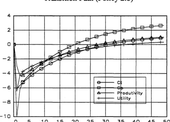
The first policy changes the public investment share from 0.5 to 0.12 while keeping alI other parameters constant. The welfare cost in this case is 2.16. When the change in alpha is from 0.85 to 0.9, modeling recent U.S. experience ( simulation one.b), the welfare cost is 1.14% of present value of output. Those values are considerable lower than the welfare costs of the corresponding steady-state policy. In both cases the reason is that utility approaches the new steady state from above. This is clear from figure seven below which measures the percentage chance in the variable in question from the original steady state. Utility rises initially and up to the fifteenth period is larger than the previous stationary leveI. The reason is that govemment consumption ( not displayed in the graph) rises initially due to the increase in alpha, and compensates the fall in private consumption. Later, with the continuous reduction in output and tax collection, public consumption ends up also falling, but never below the original steady-state leveI. Note also the continuous drop in labor productivity .
Q) 5
...
c...
(J') >.o
"'C C Q)...
-5 (J') c c -10 OI • i:: o -15 E o I.... -20-
Q) OI c -25 c ..c U N -30Figure 7:
Transition Path (Policy 1)
re-
~
t---=~
\
1:~ 13-.s '-=.. ~ I,..., ,...,'~
~
~ ~ ~~
L tilityA
il...
Cp Froduti ,itvI
~
~~
r-+--
~ ~ .~ ~ "-A~
P-s-
fs...c.
~ -.:::;ro
5 10 15 20 25 30 35 40 45 50 PeriodsSimulation two reproduces the conservative-style policy of the previous section: the share ofpublic consumption increases from 0.88 to 0.91 and capital tax decreases from 0.5 to 0.45. In this case, the total welfare cost is 0.23, almost the same as in the steady-state simulations. For this policy, steady-state income did not change much, going from 0.2611 to 0.2602 (less than 0.4%), while private consumption actualIy increased from 0.1539 to 0.1546. The drop in welfare is due, for the steady state case, to the fact that public consumption falIs proportionally more than private consumption rises, so that total consumption decreases3 . The welfare cost is higher in the present case because income and consumption first falI and then converge to the new steady state from below.
To emphasize the drawbacks of such conflicting measures (lower capital tax and lower alpha) and the necessity of fine-tuning the parameter change, simulation two.b exacerbates the parameter change, alpha now going from 0.15 to 0.1 and tk from 0.5 to 0.4.
3 Note that if ~ were set to be smaller than one so that individuaIs did not value public consumption at the same weight as private consumption, the final outcome of the present simulation might well be an increase rather than a reduction of welfare.
..
Figure 8 below displays the percentage change of selected variables with respect to the original steady state. Although utility and total consumption increase in the steady state, there is a welfare loss ofO.04 in tenns ofpresent value ofGNP when the transition path and long-run effect are taken into account. Immediately after the policy change, private consumption, total consumption and attained utility fall from the original steady state by 9%, 6.1 % and 6.4%, respectively. The convergence is not only from below but its pace is very slow in this case with private consumption taking 20 quarters to finally surpass the original steady-state levei, while attained utility takes almost 40 periods. AlI the long-run gains from the smaller capital tax are canceled out by the temporary drop in consumption and utility due to the reduction in alpha. The reason is that capital adjusts much slower than public investment, so that the reduction of the latter has short-run effects that, because of discounting, surpass the long-run effect ofhigher physical capital.
o c CTl lo..-o E o lo..- '+-Q) CTl C o .c U 4 2 o -2 -4 -6 -8 -10
Figure 8:
Transition Path (Policy 2. b)
,..., ..t:+
-~
~ 1-~
A .A...,.
~j;~
Ilr-~ ~l\~
~
r
~!J
po ~ c { ~ P oduti ity U ilityo
5 10 15 20 25 30 35 40 45 50 PeriodsAs expected, tax changes by themselves bring sizable welfare effects. In Simulation four.b only capital tax is modified. It rises from 0.4 to 0.5 and the welfare cost is 1.03.
•
However, when we keep steady-state revenue constant, by decreasing the labor tax trom 0.24 to 0.23 ( Simulation four), the welfare cost is now only 0.133. This is well below the welfare cost trom comparable steady-state exerci se, which was 5.32. As in Simulations one and one.b the reason is that the series converge trom above to the new steady-state. The relevant point, however, still is that although the new tax-mix induced a long-run increase in output while keeping revenue constant, welfare did not improve but declined. Govemment size ( total taxes in this mo dei) must decline for welfare to increase, or capital taxes must decrease and labor taxes increase.
Simulation 3 is what was called a liberal-style policy in the last section: the public investment share goes trom 12% to 24% and the capital tax rate goes trom 0.5 to 0.45. The effect over the economic series of this policy is displayed in figure 9 below.
Q} 16
....
o....
(/) >-~ o Q}....
(/) 8~
~ ... o c 01 '-o
(;
,~ ',...., E O o ~-
Q} 01 \,.... ,.... '-' C o ..c. U ~ -8 O 5Figure 9:
Transition Path (Policy 3)
-
K-
H-
Y Uti lity """ ~ '" .A. '" I""" ~ ~ Cp ... ...., ... ~ A JI.. A A A A A A A-
1 --
-
~ ..., ... ,..., ,..., ..., ..., ~ ~ ~ ~ ~-
-
- - - -
~ ~ ~ ~ ~ ,.... ... ,.... ,.... ... ,.... ,.... ,.... ... ... ... ... ~-
...., ~ I~-
-
--
~ 10 15 20 25 30 35 40 45 50 Periods•
..
'"
•
The first thing that catches our attention is the fast convergence as opposed to simulation three.b. In less than four quarters most of the series are very close to the new steady state. Also, given the relative magnitude of the change in parameters, hours worked (after an initial reduction) as well as consumption, labor productivity ( not displayed in the graph) and attained utility increase. We could expect that ifthe change in alpha were smaller and/or the increase in 'tk larger, the opposite might happen, as higher tax rates induce a reduction in these variables. As a matter of fact, capital stock falls with this policy change as expected. Nonetheless, output increases as the effect of higher hours and public investment dominates. Finally, the welfare gain of the present policy change is 0.89, as both consumption and utility rise, but it is smaller than the gain from the comparable policy for the steady state.
6 Conclusion
This paper addressed the welfare and macroeconomic effects of fiscal policy in a modified real business cycle framework where govemment not only chooses the tax rates but also the distribution of revenues between consumption and investment. The model is set such that public consumption affects individuals' utility, and public capital is part of the productivity process as a separate argument of the production function.
The policy simulations suggest that the larger the proportion of investments out of total public expenditures the larger the equilibrium leveI of capital stock, hours worked and output. It also increases labor productivity indicating that part of the slowdown of productivity growth in the seventies and eighties can be explained by the slowdown in public investment observed in this period. We showed that when investment goes trom 12% to 13% of public expenditures, labor productivity increases by 1.2%. In addition, reallocating expenditures to investment also induces higher attained utility leveis: the increase in output leads to higher private consumption and also public consumption, as the larger tax revenues offset the effect of the decrease in the proportion of public consumption in total govemment expenditures. Note that this result implies that the slowdown of public investment in the seventies and beginning of the eighties brought about sizable welfare losses to the V.S. population.
The effect of tax changes depends on the magnitude of the public-expenses elasticity of output. For large enough elasticities, increases in both the capital and labor tax rates can actually lead to increases in the capital stock and output. The effect on returns due to higher
)
•
t
..
-
..
public investment (boosted by the enlarged tax revenues) overcomes the reduction on returns due to the larger tax rates. For smaller elasticities, the distortionary effect dominates, and the usual neoclassical result of higher tax leading to smaller output and capital stock prevails.
The welfare exercises point to the fact that there is much to be gained merely by increasing the share of investment in total public expenditures. However, recent policy proposals that add tax increases to this need careful fine-tuning, otherwis~ what is gained by higher proportional investment is lost because of the increase in taxation.
Another important result indicates that govemment can be tempted to mcrease consumption while cutting tax because of run welfare gains. Govemments are short-lived and although the long run outcome at present value represents a welfare loss, the political benefits of 4 or 8 years of increased consumption could well decide in favor of this kind of policy. One of our next goals is to study in greater depth this type of trade-off in environments where policies are endogenous .
r
•
..
..
References
Aschauer, D., (1989) "Is Public Expenditure Productive?" Journal ofMonetary Economics, 23, March, pp. 177 - 200.
Barro and X. Sala-i-Martin, (1993) "Public Finance in Models of Economic Growth" , Review ofEconomic Studies, 59, pp. 645 - 661.
Barro, Rl, (1990) "Governrnent Spending in a Simple Model of Endogenous Growth " , Journal of Political Economy, 98, pp. S L03 - 25.
Baxter, M. and R King, (1993) "Fiscal Policy in General Equilibrium", American Economy Review, 83, pp. 315 - 334.
Christiano, L.l (1988) "Why Does Inventory Investment Fluctuate So Much?" Journal of Monetary Economics, 21, pp. 247 - 80.
Cooley, T. F. and G. D. Hansen (1989) "The Irrflation Tax in a Real Business Cycle Model", American Economy Review, 79, pp. 733 - 48.
Cooley, T. F. and G. D. Hansen (1992) "Tax Distortion m a Neoclassical Monetary Economy", Manuscript, Rochester University.
Ferreira, P.c. (1993), "The Impact of Public Investment and Public Capital on Economic Growth: an Empirical Investigation", Manuscript, University ofPennsylvania.
Greenwood, l, Hercowitz, Z. and P. Krussel (1992) "Macroeconomic Implications of Investment-Specific Technological Change", Manuscript, University ofRochester.
Hansen, G.D. and E.C. Prescott (1993) "Did Technology Shocks Cause the 1990-1991 Recession?" Manuscript, Federal Reserve Bank ofMinneapolis.
Hansen, G.D. and E.C. Prescott (1995) "Recursive Methods for Computing Equilibria Business Cycle Models", in Cooley, T.F. (org) Frontiers of Business Cycle Research, Princeton University Press.
Holtz-Eakin, D. (1992), "Public Sector Capital and Productivity Puzzle", NBER Working Paper # 4122.
Hulten, C. and R Schwab (1992), "Public Capital Formation and the Growth of Regional Manufacturing Industries", National Tax Journal, vol. 45, 4, pp. 121 - 143.
Kydland, F. and E.C. Prescott (1982) "Time to Build and Aggregate Fluctuations", Econometrica, 50, pp. 173 - 208.
•
Morrison, C. 1. and A. E. Schwartz (1992) "State Infrastructure and Productive Performance", NBER Working Paper nO 398l.
Nadiri, M. I. and T.P. Manuneas (1992), "The Effects of Public Infrastructure and R&D Capital on the Cost Structure and Performance of US Manufacturing Industries",
Working Paper: New York University .
, Prescott, E. C., (1986) "Theory Ahead of Business Cycle Measurement", Federal Reserve • Bank of Minneapolis Quartely Review, 10, 9 -22 .
...
•
: i
1
MARIO HENRIQUE SIMONSEN
N.Cham. P/EPGE SPE F383we
Autor: Ferreira, Pedro Cavalcanti.
Título: We1fare and fiscal policy with public goods and
1111111111111111111111111111111111111111