Modeling the creep behavior of GRFP truss structures with
Positional Finite Element Method
Abstract
This paper presents the development of a formulation, based on Positional Finite Element Method, to describe the viscoelastic mechanical behavior of space trusses. The numerical method used was chosen due to its efficiency in the applications concerning nonlinear numerical analyses. The formula-tion describes the posiformula-tional variaformula-tion over time under constant stress state (creep). The objective is to provide a way to quantify the creep be-havior for space truss structures and thus contribute to the encouragement of GFRP usage in such structural components. Time-dependent behavior of such materials is one the most important factors for their use in design of structures, demanding studies about the deformations expected within the operational life of the structural systems. To perform this study, the pro-posed methodology considers a standard solid rheological model to de-scribe stress-strain time-dependent law. This model is implemented in the formulation for quantify the total strain energy. The effects of the model parameters in the mechanical response of the structure with accentuated geometric nonlinearity were presented. In this analysis, it was possible to identify the influence of the elastic and the viscous moduli on the creep re-sponse. Model calibration was performed using test data obtained from lit-erature and a GFRP transmission line tower cross-arm was simulated to predict the evolution of displacements under real operational loads. From the results, it was possible to observe a fast evolution of displacements due to the creep effect in the first 7,500 h. This increase was close to 0.6% in relation to the displacement obtained in the elastic behavior. The present-ed methodology providpresent-ed a simple and efficient way to quantify the creep phenomenon in viscoelastic GFRP composites truss structures, as can be seen in the developed analyses.
Keywords
Creep, Positional Finite Element Method, Rheological Model, Nonlinear Analysis, GFRP.
1 INTRODUCTION
Composites have great potential to be employed in the field of Civil, Mechanical, Maritime and Aeronautical Engineering. Specific characteristics, such as high stiffness and strength, associated with low specific weight make their use very attractive, compensating the higher costs of production.
Glass Fiber Reinforced Plastics (GFRP) have been widely used in construction of structures, replacing the usual steel elements, particularly in truss structures such as electrical transmission lattice towers. These materi-als are essentially composed of glass-fibers embedded in a resin matrix polymer. GFRP prismatic components can be manufactured with different cross sections via the process of pultrusion, in which the fibers are wetted in a viscoelastic matrix (resin) and subsequently pulled through a die for compacting and curing.
Specific properties of these materials make them advantageous to be considered as an alternative to the usu-al metusu-allic materiusu-als. For instance, proprieties such as electricusu-al and magnetic insulation, controllable thermusu-al expansion, fatigue strength, damping characteristics, high strength-to-weight ratio and adequate tensile and com-pression strengths make GFRP a competitive material to be used in some applications to replace the usual steel components (Benmokrane et al., 1995). Furthermore, GFRP can be easily subjected to recycling: the waste could be incorporated, for example, into based mortars, as sand aggregates and filler replacements, which is a benefit to
João M. G. Rabelo a* Juliano S. Becho a Marcelo Greco a Carlos A. Cimini Jr. a
a Universidade Federal de Minas Gerais (UFMG),
Escola de Engenharia, Programa de Pós-Graduação em Engenharia de Estruturas. Belo Horizonte, MG, Brazil. E-mail: [email protected], [email protected],
[email protected], [email protected] *Corresponding author
http://dx.doi.org/10.1590/1679-78254432
Received: August 26, 2017
These characteristics make GFRP an excellent candidate for Transmission Line Towers (TLT). Selvaraj et al. (2012) and Selvaraj et al. (2013) developed experimental studies on X-braced panels made from GFRP pultruded sections and also on a composite cross arm for TLTs, encouraging the use of GFRP structural profiles as an alter-native material for steel members. The use of GFRP demonstrated to be efficient in reducing the hallway practiced in India for power utilities. Godat et al. (2013) also investigated the replacement of traditional materials (steel, wood and concrete) in TLTs by fiberglass pultruded members, leading to a better understanding of the behavior of GFRP in such structures. They analyzed the behavior of GFRP angle, square, rectangular, W and I sections under axial load. According Godat et al. (2013), the generalized buckling appears at low stresses and prevents FRP (Fi-ber Reinforced Plastic) profiles to reach their full-strength capacity. Izumi et al. (2000) developed a type FRP insulation arm for a 154 kV line post and tested it for mechanical and electrical performance. Yeh and Yang (1997) and Yeh and Yeh (2001) studied the feasibility of building a transmission tower from a composite material and indicated the need to look into the important aspects of creep.
One of the challenges faced in utilizing the GFRP designs is to evaluate the strains of pultruded elements un-der constant loading during the life of the structure. This time-dependent phenomenon, known as creep, is not simple to characterize and to quantify. The viscoelastic properties are of extreme importance, especially in the study of vibration damping (Melo and Radford, 2003), displacements and failure (Sá et al., 2011a; Sá et al., 2011b) of structures. Numerical techniques and analytical models have been employed, since experimental tests require long periods and are therefore costly.
Regarding the creep phenomenon, according to Benmokrane et al. (1995) and Ascione et al. (2012), in the creep behavior of GFRP strains due to viscoelastic effects are mainly caused by the resin, i.e., strains related to glass fibers are negligible, and further, the volume and the orientation of fibers have a great influence.
Some examples of techniques applying rheological formulations implemented in numerical models can be found in the specialized literature to predict the time-dependent behavior of these materials. Sá et al. (2011a) and Sá et al. (2011b) proposed a formulation considering the Maxwell rheological model and two rheological Kelvin models connected in series (Bruger-Kelvin model) to express the viscoelastic behavior of an I-section beam. This model, when compared with the experimental data, presented a similar behavior up to the first 1,000 h. Argyris et al. (1991) and Argyris et al. (1992) developed an appropriate numerical model using rheological models of Max-well and Kelvin-Voigt for the analysis of membrane structures in PVC-coated fabric. Fritsch et al. (2009) devel-oped a novel rheological material model that features a decomposition of the stress into a time independent qua-si-static component and a time and strain dependent viscous component, correctly reproducing the quaqua-si-static and dynamic stress-strain behavior of the fiber-reinforced polypropylene. Kaliske (2000) introduced an aniso-tropic constitutive formulation discretized into finite elements, using the generalized Maxwell model for applica-tion to transversely isotropic materials, performing static and dynamic analyses of U and laminates profiles, and extending the application for mechanical biology. Ascione et al. (2012) presented a program of creep tests to vali-date a mechanical model (based on Maxwell and Kelvin-Voigt rheological models) formulated for the analysis of viscous properties of FRP laminates.
Other recent works related to viscoelastic behavior, focused on the development of numerical formulations, adopt different rheological models and confirm the relevance and actuality of the theme.
Panagiotopoulos et al. (2014) use a formulation based on the Boundary Element Method for the analysis of three-dimensional solids to compare the responses of the Hooke, Kelvin-Voigt and Boltzmann solid models, which respectively represent the instantaneous elastic, the damped elastic and the creep behaviors. Besides these, the responses of the fluid models of Maxwell, Jeffreys and Burgers were also implemented and compared.
Kühl et al. (2016) propose a formulation based on integral equations to describe the nonlinear viscoelastic behavior of High Density Polyethylene (HDP). For the viscoelastic part of the strain, a generalized model of Kel-vin-Voigt is adopted, and for the viscoelastoplastic part the equation of Zapas-Crissman was considered. The vis-coelastic parameters are obtained through a curve fitting based on the method of Particle Swarm Optimization, whereas the viscoplastic parameters are obtained through a linear regression of the Least Squares Method.
Pascon and Coda (2017) propose an alternative solid finite formulation for large deformations analysis of viscoelastic materials. In this alternative methodology the neo-Hookean hyperelastic law is taken into account together with the standard solid rheological model. This new approach is based on positions and can be used to reproduce creep, stress relaxation and viscoelastic rate dependent stiffening at large strains, which are usually observed in polymeric materials.
The present paper proposes a model for the analyses of creep phenomenon in viscoelastic composites truss structures. For this purpose, a positional formulation of geometrical nonlinear analysis is used to introduce the rheological model and describe the behavior of viscoelastic materials in structures with time. The objective is to provide a simple and efficient way to quantify the creep behavior for space truss structures and thus contribute to the encouragement of the use of GFRP in such structural components. As an application example, it is presented the calibration of the model based on experimental tests performed by Youssef (2010) at different stress levels and the simulation of the time-dependent deformation evolution resulting from the viscoelastic effect for a typical structure of a power TLT cross-arm.
2 VISCOELASTIC COMPOSITE MATERIALS AND CREEP PHENOMENON
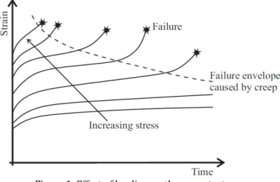
In general, polymeric matrix composites present viscoelastic behavior. This time-dependent behavior of such materials is one the most important factors for their use in design of structures, demanding studies about the deformations expected within the operational life of the structural systems. It is important to notice that fiber-matrix slippage may occur due the viscosity of the resins employed, causing additional plastic deformation over time (Scott et al., 1995). This viscoelastic behavior is a consequence of the Second Thermodynamics’ Law accord-ing to which a portion of the imparted energy of deformation is always dissipated as heat by viscous forces even while the rest is resiliently stored. Thus, once the material is loaded for a defined finite time, there is no return to its original position and permanent deformations occur. The process is neither instantaneous nor infinitely slow: it is a gradual process (Christensen, 1982). This phenomenon depends on the duration of loading and the envi-ronment conditions that structures are subjected, affecting their functionality and durability. Manufacturing con-ditions and exposition to temperature changes, pressure and humidity are examples that can affect the viscoelas-tic behavior of materials. The loading conditions can also interfere in the proprieties, and high stresses levels can lead to rupture by creep over time (Figure 1).
Figure 1: Effect of loading on the creep test.
The viscoelastic behavior sits between two extremes: purely elastic materials and purely viscous materials. However, for the developed model in this work, the contribution of the material plastic deformation due to the viscosity of it is not taken into account. All the strain attained in the loading procedure can be slowly recovered after the structural unloading.
Macro-mechanical theories concerning the viscoelastic behavior of FRP composites have attempted to pre-dict the behavior of these materials. For example, two theories are already consolidated: Findley power law, that describe the time-dependent behavior of FRP composites under a constant stress (Findley et al., 1976), and Schapery single integral equation (Schapery, 1969), that uses the principles of thermodynamics to describe the viscoelastic response of many polymers by four stress-dependent parameters. A thorough review on the creep phenomenon is performed in Scott et al. (1995).
es-strength. Therefore, it is possible to observe that there is a need to study this phenomenon in more detail and to consider the effect of creep in the design of composites structural components.
3 NONLINEAR POSITIONAL FORMULATION FOR VISCOELASTIC SPACE TRUSS ANALYSIS
The positional formulation of the Finite Element Method used for this paper is based on the formulations found in Coda and Greco (2004) and Greco et al. (2006). The method was selected due to its efficiency in the ap-plications and developments shown in recent published work concerning nonlinear numerical analysis (Car-razedo and Coda, 2010; Jian et al., 2012; Ma et al., 2012). It is supported by physics principles based on energy equilibrium that are both consistent and easy to understand. This formulation considers the nodal positions of a structure as variables, rather than nodal displacements, regarding a system of reference fixed in the space in or-der to describe the kinematics of the finite elements. The position description makes use of an intermediate non-dimensional space that enables the determination of a non-linear “engineering” strain calculated from a relative unitary length for different positions in the structure (Coda and Greco, 2004).
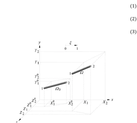
A geometric nonlinear formulation for the analysis of truss structures using spatial bar finite elements is fur-ther described. The kinematics of this adopted element can be seen in Figure 2.
This kinematics can be parameterized as a function of a non-dimensional variable ξ, that assumes values be-tween 0 and 1. Note that X1, Y1 and Z1 are the coordinates of the initial node and X2, Y2 and Z2 the coordinates of
final node of the bar finite element (Figure 2) and represent its six degrees of freedom. It is possible to write the parametric equations of the element as:
1 2 1
x X
X
X
(1)
1 2 1
y Y
Y Y
(2)
1 2 1
z Z
Z Z
(3)Figure 2: Parametrization of a bar element for trusses geometric configuration (Ω0 is the initial configuration and Ω is
the deformed configuration). Assuming ds as an infinitesimal linear dimension calculated by:
2 2 2
ds
dx
dy
dz
(4)the differential of ds in terms of ξ can be written as:
2 2 2
2 2 2
2 1 2 1 2 1
ds
dx
dy
dz
X
X
Y Y
Z
Z
l
d
d
d
d
(5)By varying the length of the element caused by the deformation of the structure it is possible to determine the Total Strain Energy U accumulated for each structural element. The term U is described by the integral of the deformation energy in a volume element, the Specific Strain Energy (u), which considers viscoelastic effects:
V V
U
udV
d dV
(6)where σ is defined as the Cauchy stress and ε is the engineering strain measure. The strain energy is assumed to be zero in a reference position or non-deformed position of the structure (Coda and Greco, 2004).
3.1 The standard solid rheological model
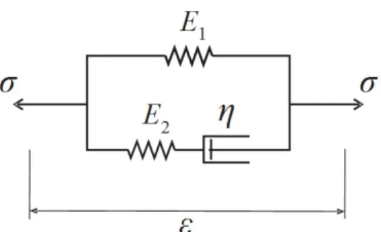
It was considered the standard solid rheological model to take into account the viscoelastic behavior of the material. This model is formed by the association of two elastic elements and one viscous element (Marques and Creus, 2012), as shown in Figure 3. The model describes the rheological law which relates stress, strain and time.
From Figure 3 it is possible to assume the following relations (Equations (7) and (8)) for the total stress and strain, respectively:
1 2
(7)1 2 2e 2v
(8)Figure 3: Standard solid rheological model (uniaxial representation).
The subscripts ()1 and ()2 refer to the path 1 (elastic element) and path 2 (elastic and viscous elements) of
the model (Figure 3) and the superscripts ()e and ()v refer to the elastic and viscous components, respectively.
The required terms of Equations (7) and (8) are given by:
1
E
1
(9)2 2e 2v
(10)2 2
2 e e
E
(11)2 2
2 v v
(12)where E1, E2 and η are physical parameters of elements presented in Figure 3 and represent the mechanical
properties of the material.
Deriving the Equation (8) as a function of time, combining the terms obtained by Equations (11) and (12), and considering the time-independent elastic modulus, results in:
2 2
2 2
E
(13)1 1 2 2
E
E
E
(14)and rearranging the terms of Equation (14) for σ, follows:
2 1 2 2
1
2 2
(
E E
)
E
E
E
(15)Equation (15) represents the rheological relation, which describes viscoelastic mechanical behavior of the model.
Considering the used nonlinear formulation, the total strain ε can be written as follows:
0
1
B
l
(16)where l0 is the initial length of the element, and B is defined as:
2
2
22 1 2 1 2 1
B
X
X
Y Y
Z
Z
(17)It is important to note that the positional formulation considers the nodal positions as variables of the prob-lem while the rheological relation is a function of the deformation rate. Thus, by using the chain rule, the strain rate
of the structure is replaced by the product between the derivative of the strain with respect to the nodal parameters of the positional formulation and the rate of variation of these parameters, as follows:,
i i ix
x
x t
(18)where
x
i represents the velocity of positional variation of the finite element in each degree of freedom. An auxiliary variable,x
axial, can be used to describe the length variation of the finite element at a time variation ∆t, as described by the following expression:
2 2 2
1 1 1 1 1 1
2 1 2 1 2 1
2 2 2
0 0 0 0 0 0
2 1 2 1 2 1
1
t t t t t taxial
t t t t t t
x
X
X
Y
Y
Z
Z
t
X
X
Y
Y
Z
Z
(19)where 1 1t
X , 1 1t
Y , 1 1t
Z , 1 2t
X , 1 2t
Y , and 1 2t
Z are the positions in the current instant moment and 0 1t
X , 0 1t
Y ,
0 1t
Z , 0 2t
X , 0 2t
Y , and 0 2t
Z are the positions in the previous instant. Thus, the terms of the velocity of positional
variation in each degree of freedom can be obtained by means of an appropriate matrix of transformation from the local (axial) system to the global system.
3.2 The deformation described in terms of time variable
The rheological model for the viscosity analysis of structural systems and the development of the positional formulation for the deformation described in terms of time variable is following presented. Rewriting Equation (6) using Equation (15):
1 2 1 2 2
(
)
VE E
U
E d
d
d dV
E
E
(20)
2 2 2
1 2
1 1
2
2 2
0 0 2 0 0 2
,
,
1
1
2
i4
i i i e i4
i i iV X X
E E B
B
E
B
B
E
U
x dX
x dX dV
l
l E
B
l
l E B
(21)Considering the cross-section area (A) invariant, and a simple mapping in the dimensionless variable ξ do-main, it is possible to achieve the integration of Equation (21) along the length of the finite element, as follows:
2 2 2
1 2
1 1
0 2 2 2
0 0 2 0 0 2
,
,
1
1
2
i4
i4
e
i i
i i i i
X X
E E B
B
E
B
B
E
U l A
x dX
x dX d
l
l E
B
l
l E B
(22)Equation (22) can be rewritten in a compact form;
1 0 0 l
U
l u d
(23)where the variable ul is a term associated with the specific energy of deformation per unit of length.
For a conservative structural problem associated with a reference system fixed in space, it is possible to write the stationary Total Potential Energy (П) as a function of the Total Strain Energy (U) and the Potential En-ergy of Applied Forces (P) acting on each node of a finite element, as follows:
Π U P
(24)The principle of Minimum Potential Energy is applied, in which the equilibrium of the structure will occur when the differential of the Total Potential Energy (П) for each degree of freedom of the structure is equal to 0, i.e., when the change rate of the Total Potential Energy is equal to zero. Writing in indicial notation (i = 1, 2, ..., 6):
1 0
0
l o i i iu
Π l
d
F
X
X
(25)The Equation (25) represents a system with six equations whose adopted solution consists in a numerical strategy in which the derivatives are developed within the integral and analytically integrated for the dimension-less variable ξ. It can be noticed that the resulting numerical integral is nonlinear for the nodal positions and cor-responds to a system of six equations by finite element due to its the six degrees of freedom (Greco et al., 2006). Therefore, the system of Equation (25) can be written using indicial notation (free index i = 1 to 6 and dummy index j = 1 to 6):
( , )
( )
0
i j i i j i
i
Π
g X F
f X
F
X
(26)or in a tensor representation:
( )
0
i i i
g X
f F
(27)Note that, in this study, the applied forces are independent of coordinates (i.e. conservative forces). The vec-tor function gi(X) is nonlinear regarding the nodal parameters. To solve Equation (27), the Newton-Raphson
pro-cedure can be used (Kleiber, 1989):
0,
00
i i i k
g X
g X
g
X
X
(28)where X is any nodal position and X0 is the initial nodal position.
The iterative Newton-Raphson process is summarized as follows (Greco et al., 2006):
1) Assume X0 as the initial configuration. Calculate gi(X0) by Equation (29):
0 1
0 0 0
( )
,
i l i X i
g X
l u d
F
(29)0 1
0 0 0
, ( )
,
i k l ik X
g
X
l u d
(30)3) Solve the system of Equation (28) and determine ∆X.
4) Update position X0 = X0 + ΔX. Return to step (1) until ΔX to be less than the tolerance.
3.3 Necessary algebraic development
To implement this formulation, the variables involved must be numerically determined, thus, the term l0ul of
Equation (23) is rewritten as:
2 2 2
1 2
1 0 1
0 0 2
0 0 2 0 0 2
,
,
1
1
2
i4
i e i4
il i i i i
X X
A E E
E Al
B
B
B
AE
B
l u
x dX
Al
x dX
l
l E
B
l
l E B
(31)The first derivative of Equation (31), related to the nodal parameter i, is expressed by:
2 21 2 2 1
1 0
0 2 0 0 2
,
,
,
,
,
1
2
4
2
4
e
i i i i i i
l i
E E
B
B x
A B
AE B x
E A
B
A
l u
l
E
l
B
l E B
B
B
(32)Analogously the derivative of Equation (32) related to the nodal parameter k is given by:
1 2 1 0 0 2 2 2(
) ,
A
,
2 ,
1
, ,
2 ,
, ,
, ,
4
2
,
,
, ,
,
i
l ik ik i k ik i i i k i k i
o
e e
i k i k ik
E E B
E
B
l u
BB
B B
BB x BB x
B B x
B
B
l
Bl E
BB
B B
BB
B
(33)With these equations and the iterative Newton-Raphson process, all of the terms required for obtaining the nodal parameters X1, Y1, Z1, X2, Y2 and Z2 can be calculated, taking into account the effects of viscoelastic behavior.
Thus, it is possible to define the equilibrium positions of a truss structure of GFRP over time by adopting suitable material parameters (E1, E2 and η). These parameters for describing the viscoelastic behavior can be obtained by
calibrating the proposed formulation by means of experimental results of traction creep tests of GFRP bars. It should be noted that no coordinate transformation was performed using this formulation, since no local coordinate systems are used. Therefore, the derivatives are calculated in a single coordinate system. Normal loads acting on the elements can be calculated by the Cauchy equation (Greco et al., 2006).
4 NUMERICAL EXAMPLES AND ANALYSIS OF RESULTS
For the analyses presented, two assumptions were adopted. The first is that the rate of stress
in Equation (15) is set equal to zero. This approximation is valid for the study of creep behavior, in which the stress is kept constant over time. For relaxation, this assumption is not valid because, in this case, the deformation is taken as constant and the stress is varying in time. The second refers to the elastic parameters shown in Equation (34). It is assumed that the sum of the modules E1 and E2 is always constant and represents the material longitudinalelasticity modulus E.
1 2
E E E
(34)4.1 Analysis of viscoelastic parameters
Figure 4: Truss geometry (dimensions in m).
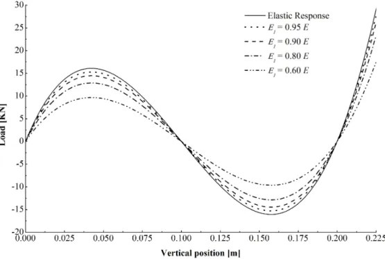
A variation in the elastic modulus E1 was considered in the first case. Figure 5 presents the results obtained
for the labeled node where the prescribed position was applied. It can be noted that as the elastic modulus E1
decreases, the force required to achieve the same position is smaller. This follows from the simple fact that the effect of this viscoelastic parameter causes a lower structural stiffness and therefore the structure comes into instability to a lower stress level. The elastic curve is represented by E1 = E, i.e., without considering the viscosity
of the material. The other fixed parameters used were A = 0.0009 m2, E = 46.9 GPa, η = 10.0 GPa·s and Δt = 100 s.
In the second case, a variation in the viscous modulus η was considered, while the elastic moduli, E1 and E2,
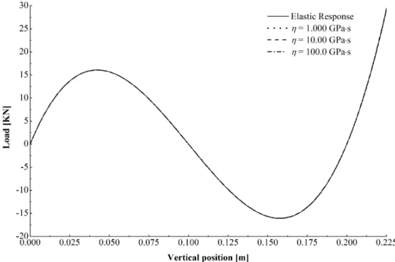
were kept respectively fixed as 0.999 and 0.001 of the material longitudinal elasticity modulus E. Furthermore, the other parameters were considered the same as in the previous case. Figure 6 presents the results obtained for the node where the prescribed position is applied. The elastic curve was represented with η tending to infinity, i.e., the dashpot was considered as a rigid bar in the rheological model. Figure 7 is a detail of Figure 6, magnifying the region of the snap-through first peak. It is possible to note that the variation in the viscous modulus causes slight changes on the obtained results, mainly due to the influence of the viscous modulus on the velocity to obtain the equilibrium position for a given applied load, while the value of the equilibrium position is defined by the elastic modulus E1.
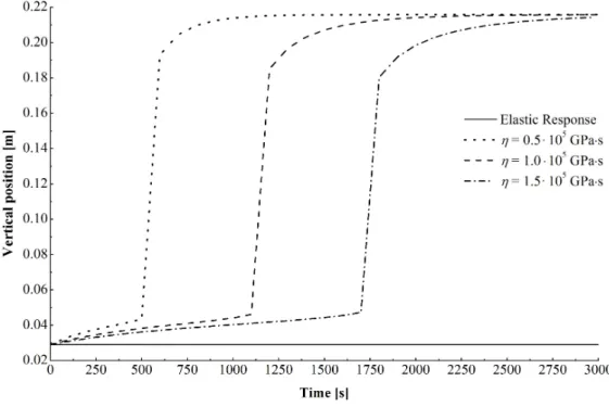
Figure 8 shows the contribution of the viscous modulus to the viscoelastic behavior, in the analysis of the same structure. In this analysis, a downward static load of P = 14.7 kN was applied and maintained constant dur-ing 30 time steps of Δt = 100 s. The elastic modules, E1 and E2, were kept respectively 0.9 and 0.1 of the material
longitudinal elasticity modulus E. The influence of the viscous modulus on the velocity to obtain the equilibrium position can be clearly seen. The equilibrium position is reached faster for lower viscous moduli materials. Fur-thermore, it is possible to notice the phenomenon of the snap-through for load levels lower than expected in the elastic snap-through behavior, considering the creep behavior.
Figure 6: Influence of the viscous modulus η on the equilibrium path (prescribed position).
Figure 8: Influence of the viscous modulus η on displacement over time.
4.2 Model calibration
In order to access the viscoelastic behavior of GFRP, a model calibration was performed based on the test da-ta obda-tained by Youssef (2010). In his work, he performed an experimenda-tal study on the creep behavior of GFRP rods for concrete reinforcement over the first 10,000 hours at different stress levels: 15%, 30%, 45% and 60% of ultimate strength. The tested bar is made of high-strength E-glass fibres (77.3% fibres by volume; 59.9% fibres by weight) impregnated in vinylester resin. The bar's circular cross section has 9.5 mm diameter; manufactured by a process that involves pultrusion with sand-coating along the external surface of the bar. The surrounding envi-ronment whilst conducting the long-term creep tests is standard laboratory atmosphere (23 ± 3 °C and 50 ± 10% relative humidity).
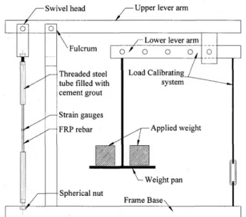
As presented in Youssef (2010), all samples were prepared according to CAN/CSA S806-02 (Canadian Stand-ards Association, 2002) and ACI 440.3R-04 (American Concrete Institute, Committee 440, 2004). The GFRP bars were cut into a variety of lengths (1170 mm, 1270 mm and 1470 mm) to fit into three different frame sizes of heights 1550 mm, 1750 mm and 1880 mm, respectively. Each one of the bar sample extremities was fitted into a 410 mm-long steel tube (grip) using Bristar 100 expansive grout. The steel pipe that grips on both ends have a 50 mm hollow portion, threaded on the inside, to screw/fit onto spherical nuts that keep the sample intact with the frame. Two Kyowa 10-mm strain gauges (120 ohm resistance and a gauge factor of 2.10) were attached on oppo-site sides at the middle of the free portion of each sample. For gauge installation, M-bond AE adhesive was used and gauges were properly aligned in the longitudinal direction of the bar.
Figure 9: Schematic of bar sustained load frame (Youssef, 2010).
Youssef (2010) noticed that the failure of the material by creep in this time range occurred for stresses close to 60% of the tensile strength of the material. The properties of the GFRP samples extracted from Youssef (2010) are shown in Table 1.
Table 1: Mechanical and geometrical properties (Youssef, 2010).
Ultimate tensile stress MPa 854
Modulus of elasticity GPa 46.9
Cross-section área m2 7.09 ·
10
5Length m 1
The calibration of the formulation was performed by obtaining the relations between the viscoelastic param-eters (E1, E2 and η) and the stress level (σ) to which the material was exposed. Thus, suitable parameters were
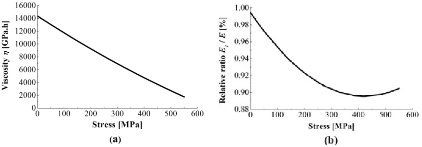
numerically adjusted to approximately match the experimental results obtained by Youssef (2010). For this, from the suitable viscoelastic parameters for each stress level, a quadratic regression was performed, using the least squares method, obtaining the following relations:
13 4 -6 2
( ) 1.4375 10
2.7127 10
7.6175 10
(35)-10 -19 2
1( ) (0.9945 4.6972 10 5.5717 10 )
E
E (36)where σ is the acting stress in Pascal (Pa). Figures 10(a) and 10(b) show the curves describing the behavior of the parameters η and E1 as function of the applied stress level σ, described respectively by Equations (35) and (36).
The results of the model calibration using Equations (34, 35 and 36)))) are shown in Figure 11, comparing the different experimental Ultimate Stress levels from Youssef (2010) with the model predictions of the strain time-depending behavior.
Figure 10: (a) Relation between the viscous modulus η and the stress level σ for GFRP material; (b) Relation between the relative ratio E1/E and the stress level σ for GFRP material.
Figure 11: Calibration of the evolution of the displacements caused by the creep phenomenon based on Youssef (2010) experimental tests.
4.3 Analyzing the viscoelastic behavior of TLT cross-arm structure
Figure 12: Cross-arm transmission line suspension tower (dimensions in m).
Table 2: Structure elements.
Bars Type of stress Cross-section area (10-4 m) stress Active
(MPa)
1, 2, 3, 4 tension 4.00 15.9
5, 6, 7, 8 compression 9.48 6.1
9, 10, 11, 12, 13, 14, 15, 16 tension or compression 2.77 < 0.1
The structure was modeled with 16 bar finite elements and 9 nodes, from which 4 are restricted, resulting in 15 degrees of freedom. The load, with magnitude of 5,394 N, is applied instantaneously in the vertical direction (negative Z axis) at the tip of the structure. It corresponds to the dead weight of the conductor cables, insulation chain, and accessories for the class of the TLT considered (138 kV lines). The cross-sections of the bars were stat-ically dimensioned for tensile loading according to the Tsai-Wu criteria (Tsai and Wu, 1971), for local buckling according to the methodology defined by Pecce and Cosenza (2000) and for global buckling according to Engesser’s equation (Zureick and Scott, 1997).
The vertical displacement at the loading node is shown in Figure 13. To generate this response, it was used Δt = 100 h and the viscoelastic parameters η, E1 and E2 obtained by Equations (34, 35 and 36)))). Table 3 shows
the value of the displacement evolution for different increasing times.
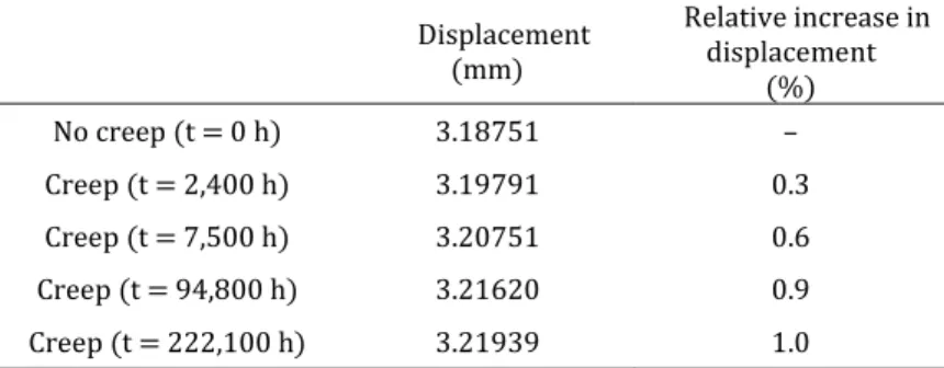
Table 3: Displacements after varied times.
Displacement (mm)
Relative increase in displacement
(%)
No creep (t = 0 h) 3.18751 –
Creep (t = 2,400 h) 3.19791 0.3
Creep (t = 7,500 h) 3.20751 0.6
Creep (t = 94,800 h) 3.21620 0.9
Creep (t = 222,100 h) 3.21939 1.0
From Figure 13 and Table 3, it is possible to observe a fast evolution of vertical displacement due to the creep effect in the first 7,500 h. This increase is close to 0.6% in relation to the displacement obtained in the elastic be-havior. After 7,500 h (~ 313 days) the evolution of displacement decreases considerably, reaching 1% only after 25 years, after which the structure is considered stable. More pronounced creep contributions can be obtained for higher stress levels, i.e., for a load of 100 kN (~ 20 times higher) an increase of approximately 9% of the dis-placement is predicted over 2,000 h (83 days). In this case, the maximum stress is 297 MPa (~ 35% of the materi-al ultimate stress).
The analysis was performed for the first 300,000 h and the results obtained are of considerable relevance for the designers to realistically access the behavior of viscoelastic structural components. However, for considerably long-time interval other aspects such as environmental conditions (moisture, temperature, radiation, etc.) must be introduced into the model to represent the behavior of the material with more reliability. Furthermore, it is important to note that the creep behavior was considered symmetric with respect to the stress level for simplifi-cation, i.e., the creep behavior for the tensile rods is equal to the compressed rods.
5 CONCLUSIONS
A formulation of geometrical nonlinear analysis was successfully implemented to analyze the creep phenom-enon in viscoelastic GFRP composites truss structures. A standard rheological model was used together to the Positional Finite Element Method to predict the evolution of deformation of viscoelastic structural components over time. The formulation was applied in a relatively simple way, since it is based on physical concepts of Total Potential Energy balance, which make it easy to understand. The viscoelastic behavior was introduced in a natural way through the implementation of a rheological relation for obtaining the Total Deformation Energy, since this relation is based on the physical behavior of springs and dashpots associations that provides equations known as phenomenological.
A parametric study was conducted to identify the influence of the elastic and the viscous moduli on the creep response of a structure with snap-through behavior. From the obtained results, it was concluded that elastic modulus is clear responsible to represent the structural stiffness. Thus, the elastic modulus decrease leads to a reduction in the force required to achieve the same position and therefore the structure presents a snap-through instability with a lower stress level. On the other hand, the variation in the viscous modulus causes slight changes on the obtained equilibrium position. This is due to the influence of the viscous modulus is mainly related to the velocity necessary to obtain the equilibrium position for a given applied load. Thus, the viscous modulus decrease leads to a reduction in the time required to achieve the same equilibrium position and, therefore, the snap-through instability phenomena can be anticipated.
In order to model the viscoelastic behavior of GFRP, a calibration of the model was performed in a simple way based on tensile creep test results obtained from the literature. The results of the calibration demonstrated fairly good approximation between numerical and experimental results.
However, special caution must be taken, because a pronounced creep contribution was obtained for higher stress levels, even though relatively less than the material ultimate stress.
Acknowledgements
The authors acknowledge the financial supports granted by CNPq (National Council for Scientific and Tech-nological Development), CAPES (Coordination of Improvement of Higher Education Personnel), FAPEMIG (Foun-dation for Research Support of Minas Gerais State) and Federal University of Minas Gerais (UFMG), under Grant Numbers 302376/2016-0, TEC-PPM-00354-14 and TEC-PPM-00409-16.
References
American Concrete Institute, Committee 440, (2004). Guide Test Methods for Fibre Reinforced Polymers (FRPs) for Reinforcing or Strengthening Concrete Structures. ACI 440.3R-04, American Concrete Institute, Farmington Hills, Mich., 40p.
Argyris, J., Doltsinis, I.S., da Silva, V.D. (1992). Constitutive modelling and computation of non-linear viscoelastic solids. Part II: Application to orthotropic PVC-coated fabrics. Computer Methods in Applied Mechanics and Engi-neering, 98(2): 159–226.
Argyris, J., Doltsinis, I.S., da Silva, V.D. (1991). Constitutive modelling and computation of non-linear viscoelastic solids. Part I: Rheological models and numerical integration techniques. Computer Methods in Applied Mechanics and Engineering, 88(2): 135–163.
Ascione, L., Berardi, V.P., D’Aponte, A. (2012). Creep phenomena in FRP materials. Mechanics Research Communi-cations, 43: 15–21.
Bahraini, S.M.S., Eghtesad, M., Farid, M., Ghavanloo, E. (2013). Large deflection of viscoelastic beams using frac-tional derivative model. Journal of Mechanical Science and Technology, 27(4): 1063-1070.
Benmokrane, B., Chaallal, O., Masmoudi, R. (1995). Glass fiber reinforced plastic (GFRP) rebars for concrete struc-tures. Construction and Building Materials, 9(6): 353–364.
Borges, A.S., Faria, A., Rade, D., Sales, T. (2017). Time Domain Modeling and Simulation of Nonlinear Slender Vis-coelastic Beams Associating Cosserat Theory and a Fractional Derivative Model. Latin American Journal of Solids and Structures, 14(1): 153-173.
Canadian Standards Association, (2002). Design and Construction of Building Components with Fibre Rei forced Polymers. CAN/CSA S806-02, Rexdale, Ontario, Canada, 177p.
Carrazedo, R., Coda, H.B. (2010) Alternative positional FEM applied to thermomechanical impact of truss struc-tures. Finite Elements in Analysis and Design, 46(11) 1008-1016.
Ciniello, A.P.D., Bavastri, C.A., Pereira, J.T. (2017). Identifying Mechanical Properties of Viscoelastic Materials in Time Domain Using the Fractional Zener Model. Latin American Journal of Solids and Structures, 14(1): 131-152.
Coda, H.B., Greco, M. (2004). A simple FEM formulation for large deflection 2D frame analysis based on position description. Computer Methods in Applied Mechanics and Engineering, 193(33): 3541–3557.
Christensen, R.M. (1982) Theory of Viscoelasticity: An Introduction. 2nd ed., Academic Press (New York).
Fritsch, J., Hiermaier, S., Strobl, G. (2009). Characterizing and modeling the non-linear viscoelastic tensile defor-mation of a glass fiber reinforced polypropylene. Composites Science and Technology, 69(14): 2460–2466.
Godat, A., Légeron, F., Gagné, V., Marmion, B. (2013). Use of FRP pultruded members for electricity transmission towers. Composite Structures, 105: 408–421.
Greco, M., Gesualdo, F.A.R., Venturini, W.S., Coda, H.B. (2006). Nonlinear positional formulation for space truss analysis. Finite Elements in Analysis and Design, 42(12): 1079–1086.
Izumi, K., Takahashi, T., Homma, H., Kuroyagi, T. (2000). Development of line post type polymer insulation arm for 154 kV. IEEE Transactions on Power Delivery, 15(4): 1304–1310.
Jian, L., Shenjie, Z., Meiling, D., Yugin, Y. (2012). Three-node Euler-Bernoulli beam element based on positional FEM. Procedia Engineering, 29: 3703-3707.
Kaliske, M. (2000). A formulation of elasticity and viscoelasticity for fibre reinforced material at small and finite strains. Computer Methods in Applied Mechanics and Engineering, 185(2): 225–243.
Kleiber, M. (1989). Incremental Finite Element Modeling in Non-linear Solid Mechanics, Ellis Horwood (England).
Kühl, A., Muñoz-Rojas, P.A., Barbieri, R., Benvenutti, I.J. (2016). A procedure for modeling the nonlinear viscoelas-toplastic creep of HDPE at small strains. Polymer Engineering and Science, 57(2): 144-152.
Ma, L.Z., Liu, J., Diao, X.L., Yan, Y.Q. (2012). The Nonlinear Static Formulation of Variable Cross-Section Beam Ele-ment Based on Positional Description. Advanced Materials Research, 557: 2367-2370.
Marques, S.P.C., Creus, G.J. (2012). Computational viscoelasticity. Springer (Heidelberg).
Meira Castro, A.C., Ribeiro, M.C.S., Santos, J., Meixedo, J.P., Silva, F.J., Fiúza, A., Alvim, M.R. (2013). Sustainable waste recycling solution for the glass fiber reinforced polymer composite materials industry. Construction and Building Materials, 45: 87–94.
Melo, J.D.D., Radford, D.W. (2003). Viscoelastic Characterization of Transversely Isotropic Composite Laminae. Journal of Composite Materials, 37(2): 129–145.
Panagiotopoulos, C.G., Mantič, V., Roubíček, T. (2014). A simple and efficient BEM implementation of quasistatic linear visco-elasticity. International Journal of Solids and Structures, 51(13): 2261-2271.
Pascon, J.P., Coda, H.B. (2017). Finite deformation analysis of visco-hyperelastic materials via solid tetrahedral finite elements. Finite Elements in Analysis and Design, 133: 25-41.
Pecce, M., Cosenza, E. (2000). Local buckling curves for the design of FRP profiles. Thin-Walled Structures, 37(3): 207–222.
Pérez Zerpa, J., Canelas, A., Sensale, B., Santana, D.B., Armentano, R.L. (2015). Modeling the arterial wall mechanics using a novel high-order viscoelastic fractional element. Applied Mathematical Modelling, 39(16): 4767-4780.
Sá, M.F., Gomes, A.M., Correia, J.R., Silvestre, N. (2011a). Creep behavior of pultruded GFRP elements - Part 1: Lit-erature review and experimental study. Composite Structures, 93(10): 2450–2459.
Schapery, R.A. (1969). On the Characterization of Nonlinear Viscoelastic Materials. Polymer Engineering and Sci-ence, 9(4): 295-310.
Scott, D.W., Lai, J.S., Zureick, A. (1995). Creep Behavior of Fiber-Reinforced Polymeric Composites: A Review of the Technical Literature. Journal of Reinforced Plastics and Composites, 14(6): 588-617.
Selvaraj, M., Kulkarni, S., Babu, R.R. (2013). Analysis and experimental testing of a built-up composite cross arm in a transmission line tower for mechanical performance. Composite Structures, 96: 1–7.
Selvaraj, M., Kulkarni, S., Babu, R.R. (2012). Structural evaluation of FRP Pultruded Sections in overhead transmis-sion line Towers. International Journal of Civil Structural Engineering, 2(3): 943–949.
Tsai, S.W., Wu, E.M. (1971). A General Theory of Strength for Anisotropic Materials. Journal of Composite Materi-als, 5(1): 58–80.
Yeh, H.Y., Yang, S.C. (1997). Building of a Composite Transmission Tower. Journal of Reinforced Plastics and Com-posites, 16(5): 414-424.
Yeh, H.Y., Yeh, H.L. (2001). A Simple Failure Analysis of the Composite Transmission Tower. Journal of Reinforced Plastics and Composites, 20(12): 1054–1065.
Youssef, T.A. (2010). Time-Dependent Behavior of Fibre Reinforced Polymer (FRP) Bars and FRP Reinforced Con-crete Beams Under Sustained Load. Doctor’s Thesis. University of Sherbrooke, Canada.