ScienceDirect
Available online at www.sciencedirect.com
ScienceDirect
www.elsevier.com/locate/procedia
Procedia Structural Integrity 5 (2017) 347–354
2452-3216 2017 The Authors. Published by Elsevier B.V.
Peer-review under responsibility of the Scientific Committee of ICSI 2017 10.1016/j.prostr.2017.07.181
ScienceDirect
Keywords: Modal analysis; vibrations; model updating
1.Introduction
This paper is devoted to characterize the dynamic properties (frequencies, modal shapes and damping) of an experimental mockup consists on a three-story structure in a shear frame configuration, which can be modeled as a three degrees-of-freedom (DOFs) structure with three lateral displacements representing the vibration of each mass.
* Corresponding author. Tel.: +351-273-303070; fax: +351-273-313051. E-mail address: [email protected]
ScienceDirect
2nd International Conference on Structural Integrity, ICSI 2017, 4-7 September 2017, Funchal,
Madeira, Portugal
Estimation of the dynamic modal parameters of a small-scaled
mockup
M. Braz-César
a*, J. Ribeiro
b, H. Lopes
caDep. of Applied Mechanics, Polytechnic Institute of Bragança, C. de Santa Apolónia, 5300- 253 Bragança, Portugal bDep. of Mechanical Technology, Polytechnic Institute of Bragança, C. de Santa Apolónia, 5300- 253 Bragança, Portugal cDep. of Mechanical Engineering, Polytechnic Institute of Porto, R. Dr. António Bernardino de Almeida, 431, 4200-072 Porto, Portugal
Abstract
This paper presents the experimental and numerical research carried out on a reduced-scaled model to obtain and simulate its dynamic modal properties. A roving impact hammer test was carried out to identify the dynamic modal properties of the structure. The measured input and output values were acquired using a Data Acquisition System (DAQ) in order to compute the corresponding Frequency Response Function (FRF) to characterize its dynamic response. Finally, the experimental results were used to optimize the parameters of a numerical model of the mockup. In this case, the model updating procedure is based on an optimization problem in which a set of parameters representing uncertainties in the modeling process of the mass, stiffness and damping is optimized to minimize the difference between the predicted and measured dynamics of the actual structure.
© 2017 The Authors. Published by Elsevier B.V.
Nomenclature
H(ω) transfer function F(ω) system input/forcing X(ω) output/response
φ mass-normalized mode vector
N number of nodes
f natural frequency in Hz X(t) displacement vector
Ẋ(t) velocity vector
Ẍ(t) acceleration vector M mass matrix K stiffness matrix C damping matrix
ẍg seismic acceleration
Г position vector
αi tuning coefficients
x vector with the updated parameters
xLB lower bound
xUB upper bound
fω(x) difference between numerical and reference frequencies
fφ(x) correlated mode shapes
ω natural frequencies in rad/s
𝛽𝛽 weighing factor (frequency)
δ weighing factor (modes)
λ weighing factor (damping)
φi experimentally measured mode shapes
φi* theoretically predicted mode shapes
ξ damping ratio
ξi experimentally measured damping ratios
ξi* analytically predicted damping ratios
I identity matrix
Modal testing represents a well-known experimental approach to study of the vibration or dynamic characteristics of mechanical systems (Ewins 1984, Schwarz and Richardson 1999). Experimental modal techniques include modal excitation techniques, Frequency Response Function (FRF) measurements processed within a Fast Fourier Transforms (FFT) analyzer, and also modal parameter estimation from a set of FRFs (using a curve fitting procedure). This paper highlights the application of a modal excitation technique with an impulse hammer to obtain the FRFs of the structural system. At first, the experimental setup of the structural model used in this investigation is presented. Then, the modal properties of the experimental model were estimated using a system identification procedure on the basis of the response to an impulse excitation. The results obtained with this procedure were then used to update a numerical model of the experimental mock-up.
2.Experimental model
columns consists of three aluminum plates with a total length of 250 mm and a rectangular cross-section of 50x1.5 mm. The diaphragm of each floor floors is made of a polycarbonate plate with 290x290x20 mm, which is monolithically attached to the columns through angle brackets. Each floor has a mass of approximately 3.65 kg and the whole mock-up has a total mass of around 19 kg.
3.System identification
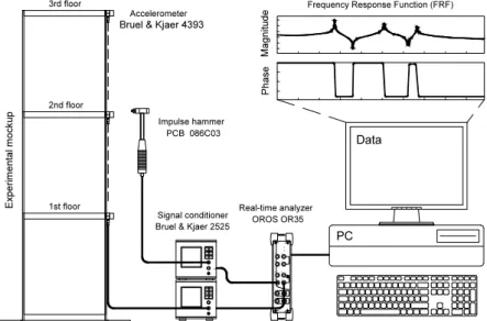
A modal analysis is carried out to obtain the dynamic characteristics of the structural model. Forced vibration testing and ambient vibration testing are two well-known dynamic system identification techniques to estimate modal parameters of civil structures. In this case, an impulse hammer test was carried out to determine the modal parameters. A schematic representation of the experimental setup used in the modal parameter estimation is shown in Fig. 1. As can be seen, the structure is excited using an impulse generated by an impact hammer at specific points on the structure. The response to this excitation is then measured together with the forcing signal. The system identification is made in the frequency domain using frequency response functions (FRF) or transfer functions H(ω) that define the casual relationship between the system input/forcing F(ω) and the output/response X(ω).
Fig. 1. Experimental setup to measure the dynamic properties of the structure.
The frequency response function may be given in terms of displacement, velocity or acceleration, which is referred as compliance, mobility and accelerance, respectively. For multiple input/output relationships, the set of FRFs between the response and the forcing function signals yields the so-called frequency response matrix Hi,j(ω). Denoting
Xii(ω) as the forcing vector and Fji(ω) as the response vector, the relationship between the force excitation (input) and
the vibration response (output) at different degrees-of-freedom (DOFs) of a linear system is given by
X ( )j i,
H ( )i j,
F ( )i i,
(1)where Hi,j(ω) is the frequency response matrix containing the FRFs between these DOFs. In this case, the frequency
response matrix of a three DOFs system is given by
,
1,12,1 1,22,2 1,32,33,1 3,2 3,3
H ( ) H ( ) H ( )
H ( ) H ( ) H ( ) H ( )
H ( ) H ( ) H ( )
i j
For lightly or proportionally damped structures, the frequency response function takes the form
, 2 2
1
1, 2, ,
( ) ( )
H ( )
1, 2, ,
( ) (2 )
N
i k j k i j
k k k k
i N
j N
i
(3)where (φi)k is the kth mass-normalized mode vector at the drive point, (φj)k is the response/output mode shape and N is
the number of modes. The modal analysis post-processing of the data was carried out through NVGate software. The frequency response functions for each input/output measurement are shown in Fig. 2 to Fig. 4.
Fig. 2. FRF magnitude and phase of H1,1.
Fig. 3. FRF magnitude and phase of H1,2.
In this case, a peak peaking method (half power method) can be used to estimate the modal properties at each peak. The dynamic parameters of the experimental mockup are listed in Table 1.
Table 1. Modal parameters of the experimental mockup.
Mode Frequency rad/s (Hz)
Damping ratio
Modal shape Modal participation
x1 x2 x3
1 12.023 (1.91398) 0.03157 -0.156 -0.218 -0.434 34.43248 2 35.354 (5.62777) 0.01198 -0.428 -0.108 0.203 35.25975 3 50.798 (8.08625) 0.00899 -0.210 0.404 -0.179 30.30777
4.Model updating
Model updating process is essentially an optimization problem that aims to update a set of parameters of a numerical model (usually, the natural frequencies and mode shapes) based on experimental data for better structural correlation results. The first step is to build a preliminary numerical model of the experimental mockup (Fig. 5).
Fig. 5. Numerical model of the three dof system under seismic excitation.
In this case the structural system is subjected to a generic earthquake ground excitation. Hence, the governing equation of motion is given by
MX( )t CX( )t KX( )t M x tg( ) (4)
where X(t), Ẋ(t) and Ẍ(t) are the displacement, velocity and acceleration vectors, respectively and M(3×3), C(3×3) and
K(3×3) are the mass, damping and stiffness matrices obtained from the geometrical and mechanical properties of the
structural elements. Finally, ẍg is the seismic acceleration and Г is a position vector.
In general, model updating techniques are based on direct or iterative methods depending on the approach used to update the parameters of the numerical model (Ewins 1984, Visser and Imregun 1991, Farhat and Hemez 1993, Mottershead and Friswell 1993, Nobari et al. 1994, Maia and Silva 1997, Rad 1997, Levin and Lieven 1998, Fritzen
et al. 1998, Carvalho et al. 2007). In this case, the updating procedure is considered as an optimization problem in which a set of parameters representing uncertainties in the modeling process of the mass, stiffness and damping is optimized in such a way as to minimize the difference between the predicted and measured dynamics of the real structure. Thus, it follows that
1 1
2 2 1 2 3 3 3
0 0
M 0 0 , ( , , )
0 0
m
m
m
(5)
4 1,1 7 1,2
7 2,1 5 2,2 8 2,3 4 5 6 7 8 8 3,2 6 3,3
0
K , ( , , , )
0
,
k k
k k k
k k
9 1,1 12 1,2
12 2,1 10 2,2 13 2,3 9 10 11 12 13 13 3,2 11 3,3
0
C , ( , , , )
0
,
c c
c c c
c c
(7)where αi represent tuning coefficients for each element of these matrices. To reduce the number of optimization
parameters, the damping can be assumed as a linear combination of the mass and stiffness matrices. Thus, the optimization problem will be formulated with the Caughey damping matrix defined as
1 9 10 11
CM K KM K (8)
The objective function also includes a cost function related with the damping coefficients. Thus, it follows that
( ) ( ) ( ) ( )
f x f x f x f x (9)
where fω(x) accounts for the difference between numerical and reference frequencies, fφ(x) is related with the correlated mode shapes and fξ(x) is related with the damping ratio. These functions are given by
2 * * 1
( ) , 0 1
N
i i
i i
i i
f x
(10)2
1
1 MAC
( ) , 0 1
MAC
N
i i
i i
i
f x
(11)2 * * 1
( ) , 0 1
N
i i
i i
i i
f x
(12)where 𝜔𝜔𝑖𝑖 and 𝜔𝜔𝑖𝑖∗ are the 𝑖𝑖th analytical and measured frequencies, respectively, 𝛽𝛽𝑖𝑖 and δi are the weight factors and ξi
and ξi* are the ith experimentally measured and analytically predicted damping ratios, respectively. MAC𝑖𝑖 represents
the 𝑖𝑖th Modal Assurance Criterion (MAC) defined as
2 * * * MAC T i i T Ti i i i
(13)
where φiand φi* are the ith experimentally measured and theoretically predicted mode shapes, respectively. Values
close to unity indicate good correlation between the between measured and predicted mode shapes while zero means no correlation at all. The optimization parameters were constrained to ensure that the resultant matrices have physical meaning and also to be compatible with the actual range of values of the experimental model (Table 2).
Table 2. Model parameters to be updated.
Num. Parameter Initial value Upper limit Lower limit
1 to 3 mi (kg) 4.50 6.65 3.65
The symmetric condition of the stiffness and damping matrices is already ensured. Besides, the eigenvector matrix (mode shapes) must be orthogonal with respect to the mass matrix. Thus, it follows that
M I
T
(14)In this case, weighting factors β= 0.4, δ= 0.4 and λ= 0.2 were selected as the reference values for the optimization process. The numerical optimization was carried out using a constrained nonlinear optimization algorithm (fmincon
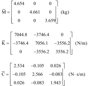
function) in MATLAB optimization toolbox. Based on these results, the updated mass, stiffness and damping matrices are given by
4.654 0 0
M 0 4.661 0 (kg)
0 0 3.659
(15)
7044.8 3746.4 0
K 3746.4 7056.1 3556.2 (N/m)
0 3556.2 3556.2
(16)
2.534 0.105 0.026
C 0.105 2.566 0.083 (N s/m)
0.026 0.083 1.943
(17)
The measured and updated FRFs are shown in Fig. 6.
The correlation between the measured data and the updated model is carried out by means of the modal assurance criterion to evaluate the effectiveness of the model updating procedure.
0.9659 0.4826 0.2466
MAC 0.6689 0.9533 0.0302
0.0282 0.0402 0.9121
(18)
The MAC matrix shows that the correlation between the updated and measured mode shapes is acceptable since all diagonal elements are close to unity (paired modes). There is however a high value in two off-diagonal elements related with the discrepancy between the experimental and analytical first and second mode shapes. The results show that there is a weak correlation between test and analytical FRFs at antiresonances. For instance, the antiresonance between the first and second natural frequency for H1,1 and H1,2 are not properly correlated.
Based on these data, there is a strong indication that the modal properties of the second DOF were not properly defined, which may contribute to the relatively large off-diagonal term in the MAC matrix. Although the model updating procedure could be improved adjusting some optimization parameters (e.g., upper and lower limits, initial value, additional constraints, etc.) or either by using a global optimization routine, the error achieved between the experimental and numerical model is relatively small. Hence, the updated model is globally satisfactory and it is assumed as being representative of the dynamic behavior of the experimental model.
5.Conclusions
This paper presents an experimental modal analysis carried out to determine the dynamic properties of a small-scale structural model. An impulse hammer test was used to determine the natural frequencies, mode shapes and also the corresponding damping ratios. An optimization procedure was implemented to update the parameters of a numerical model of the structure in order to represent the experimental system. It was found that the updated frequencies are very close to the values found with the experimental analysis displaying an error rate of less than 1% for all modes. In general, the estimated mode shapes are in line with those experimentally measured although it is visible a slight mismatch in all modes, particularly between the first and second mode shapes. Despite the slight error between the updated and measured data observed, it is assumed that the numerical model is able to represent with sufficient accuracy the dynamic characteristics of the experimental model.
References
Carvalho, J., Datta, B., Gupta, A., Lagadapati, M., 2007. A direct method for model updating with incomplete measured data and without spurious modes. Mechanical Systems and Signal Processing 21(7): 2715–2731.
Ewins, D., 1984. Modal Testing: Theory and Practice. Research Studies Press.
Farhat, C., Hemez, F., 1993. Updating finite element dynamic models using an element-by-element sensitivity methodology. AIAA Journal 31(9): 1702–1711.
Friswell, M., Inman, D., Pilkey, D., 1998. Direct updating of damping and stiffness matrices. AIAA Journal 36(3): 491–493.
Fritzen, C., Jennewein, D., Kiefer, T., 1998. Damage detection based on model updating methods. Mechanical Systems and Signal Processing 12(1): 163–186.
Levin, R., Lieven, N., 1998. Dynamic finite element model updating using simulated annealing and genetic algorithms. Mechanical Systems and Signal Processing, 12(1): 91-120.
Maia, N., Silva, J., 1997. Theoretical and experimental modal analysis. Research Studies Press, Taunton.
Mottershead, J., Friswell, M., 1993. Model updating in structural dynamics: a survey. Journal of Sound and Vibration 167(2): 347–375.
Nobari, A., Imregun, M., Rad, S., 1994. On the uniqueness of updated model. Proc. of the 19th International Seminar on Modal Analysis, Leuven, Belgium, pp. 151–163.
Rad, S., 1997. Methods for updating numerical models in structural dynamics. PhD thesis, Imperial College of Science, Technology and Medicine London, UK.
Schwarz, B., Richardson, M., 1999. Experimental Modal Analysis. Proceedings of the CSI Reliability Week, Orlando, FL.