Contents lists available atSciVerse ScienceDirect
Mathematical and Computer Modelling
journal homepage:www.elsevier.com/locate/mcmMulti-band remote sensing based retrieval model and 3D
analysis of water depth in Hulun Lake, China
Changyou Li
a, Biao Sun
a,∗, Keli Jia
a, Sheng Zhang
a, Weiping Li
b, Xiaohong Shi
a,
Claudia M.d.S. Cordovil
c, Luis S. Pereira
caCollege of Water Conservancy and Civil Engineering, Inner Mongolia Agricultural University, Hohhot, 010018, PR China bCollege of Environment & Energy Resources, Inner Mongolia Science & Technology University, Baotou, 014010, PR China cCEER - Biosystems Engineering, Institute of Agronomy, Technical University of Lisbon, Tapada da Ajuda, 1349-017 Lisbon, Portugal
a r t i c l e i n f o Article history:
Received 23 October 2012 Accepted 10 December 2012
Keywords:
Cold and arid region Inner Mongolia Lake depth Multi-band merging TIN
a b s t r a c t
Hulun Lake, a large lake located on the cold and arid Hulunbeir grassland in the Inner Mongolia Autonomous Region, is the fifth largest in China and the largest in the north of the country. However, the information on the lake’s characteristics (e.g., water depth versus surface area) is scarce in literature. Based on the lake’s physiographic features, this study developed and used a model that merges the sunlight reflection band with the thermal infrared radiation band to simulate the lake’s characteristics. The model verification and error analysis indicated an optimal model structure of logarithm. Thus, this logarithmic model was selected to analyze the spectral data. The results indicated that the model did a good job in reproducing observed water depths and accurately predicted the depths on 24 September 2007. This showed that this model can be reliably applied to the cold and arid region. Subsequently, the results were used to generate a triangular irregular network (TIN) model, which in turn was used to compute the functional relations between water level, surface area, and volume. The correlation between water level and volume is superior to that between water level and area. The regression equation developed in this study can be used to estimate the volume when water elevation is known.
Crown Copyright© 2012 Published by Elsevier Ltd. All rights reserved.
1. Introduction
Water depth, one of the basic parameters for the study of a lake environment, is conventionally measured using a positioning device mounted on a boat. The example devices are a surveying rod, plummet, ecosounding, and sonar. However, because the number of measuring points (i.e., nodes) cannot be too large and may limit conditions of field operations, the measured data have general limitations in representing the true terrain of the lake bottom. With the 3S (i.e., remote sensing, global positioning system, and geographic information system) technology advancement and maturing, its has been applied to many fields (e.g., [1–3]). One of applications is to use remote sensing to indirectly measure water depth. This indirect method uses space satellite sensors to receive the sunlight’s reflection and the self-thermal radiation of a water body. Subsequently, the satellite data are processed to retrieve water depth.
The available retrieval models can be classified into theoretical, semi-theoretical–empirical, and statistical correlation [4]. The first two types of models have not been widely used in practice because the optical parameters relevant to water body and required by those models cannot be determined and because the timings of other measurable parameters may not be coincident with those of satellite data. As a result, the current literature is dominated by researches conducted using
∗Corresponding author. Tel.: +86 13404843412.
E-mail addresses:[email protected],[email protected](B. Sun).
0895-7177/$ – see front matter Crown Copyright©2012 Published by Elsevier Ltd. All rights reserved.
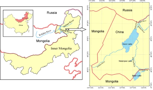
Fig. 1. Map showing the location of Hulun Lake.
statistical correlation models (e.g., [5–8]). These researches were mainly conducted for shallow seas located in humid areas (e.g., [9,10]), using images taken in summer and with wavelengths of solar radiation. In contrast, there are few research literatures about lakes in cold and arid regions, and few literatures about retrieving the water depth using the thermal infrared band. Currently, the applications about thermal infrared remote sensing are mainly concentrated on soil moisture and drought monitoring, etc. [11].
Three-dimensional terrain analysis/visualization is the new development trend of the 3S technology [12] and can more intuitively and accurately present true terrains than the information of two-dimensional data. Nowadays, the visualization is mainly applied to the fields of virtual geographic environments, digital city construction and land management and utilization, among others [13,14].
The study area was Hulun Lake located in the cold and arid region of northern China. Using the Landsat TM/ETM
+
satellite images taken in periods between late autumn and early winter and the corresponding measured data on water depth, this study developed a water depth retrieval model that merges the solar reflection band and infrared thermal radiation band. After the simulation for verification and error analysis, the bottom topography data of Hulun Lake was further calculated. The modeling results and the measured point data on the terrain were conjunctively used to generate a 3D TIN model, which to the visual operation and spatial analysis, obtain the relationships between the bottom topography of the lake and the hydrologic characteristics.2. Materials and methods
2.1. Study area
Hulun Lake, the fifth largest lake in size in China, has geographical coordinates between 116°58′E and 117°48′E and between 48°33′N and 49°20′N (Fig. 1). Towards the east are the Xing’anling Mountains and the west and south is the Mongolian Plateau. The lake has a geometric shape of an irregular oblique rectangle, with a northeast–southwest axis. The lake has a maximum length of 93 km and a maximum width of 41 km, an annual average surface area of 2054 km2, and an average water depth of about 5 m. The area is located in the semi-arid continental temperate monsoon zone, which has an annual average precipitation of 233 mm and an annual average evaporation of 1446 mm [15]. Hulun Lake is part of the Argun River water system and the majority of water is supplied by precipitation as well as by several rivers including the Kelulun River with headwaters in the Kente Mountains of the Mongolian People’s Republic, the Wuerxun River shared by Beier Lake and Hulun Lake, and the Xinkai River (nicknamed Dalaneluomu River). The Xinkai River, located in the northeast of Hulun Lake, can have dual flow directions: towards Hulun Lake when the Hailar River has a higher water level but towards the Argun River when Hulun Lake has a higher level [16].
Hulun Lake, with a large water surface area and nicknamed the ‘‘Prairie Pearl’’, is located on the Hulunbeir grassland of the Inner Mongolia Autonomous Region. The Hulunbeier grassland had plenty of water and lush grass, and is one
of the Chinese high-quality natural pastures and an important animal husbandry production base. Hulun Lake and the surrounding grasslands, totally about 7400 km2 in size, were designated a Provincial Nature Reserve in 1990, approved as a National Nature Reserve in 1992, listed by the United Nations as an International Importance Wetland in January 2002, and were nominated as a World Biosphere Reserve member by the United Nations Educational Scientific and Cultural Organization (UNESCO) Man and the Biosphere Program in November 2002 [17,18]. Along with the Hulunbeier grassland and Daxinganling forest, Hulun Lake functions as an important ecological protection barrier in northern China and plays important roles in maintaining the regional biological diversity, protecting the ecological security of northern China and even Huabei District, and promoting sustainable economic and social development [19,20]. Since 2000, because of the interactive impacts of various natural and human factors, the water supplement to Hulun Lake has become much less than the water consumption. As a result, the lake level has been dropping from year to year, which has seriously impacted the lake’s fisheries and its surrounding ecological health. This also resulted in the continuous deterioration of the Hulunbeier grassland environment. The objective of this study was to determine the water depths and the bottom terrains of Hulun Lake, providing the scientific information that can be used to develop lake protection measures.
2.2. Model principles 2.2.1. Sunlight reflection
The light radiation to a water body is either absorbed or reflected by water. As a result, the radiation tends to fade away with the increase of water depth. The radiation that reaches the lake bottom and is reflected back is subject to further losses to water absorption and reflection, and the remaining radiation will pass through the atmosphere to reach the space sensor. These processes can be mathematically described as [21]:
Li
=
Li∞+
CiRB(λ)
e−kifZ (1)where Li is the i band radiation received by the sensor; Ciis a constant dependent on solar irradiance, atmospheric and water transmittance, and water surface refraction; Li∞is the radiation into the deep water zone; RBis the reflectance at the bottom of the water body;
λ
is the solar radiation; kiis the attenuation coefficient of the water body; f is the path length of the water body (usually taken as 2); Z is the water depth.This model assumes that the light radiation received by the sensor is inversely proportional to water depth. The premises of the model are that the bottom reflectance is large and that the water is clear and shallow. These premises can impose application limitations of the model. To relax these limitations, Wei et al. [22] proposed a new remote sensing based retrieval method expressed as:
Z
= −
1 kln
1−
Li−
B A
(2) where A and B are two coefficients, which can be determined based on observed Z and Li.Based on the e exponential an optical exponential attenuation model was proposed. This model requires two or more different bands and assumes a constant reflectance at the bottom. This multi-band retrieval model is independent of the bottom geometry and expressed as:
Z
=
A0+
A1B1+
A2B2+ · · ·
AnBn (3)where Bi
=
ln(
Li−
L∞)/
ki; Aiare coefficients and can be defined by regressing measured water depths and radiation pixel values.2.2.2. Lake thermal radiation
In terms of the principle of thermal convection and because the atmosphere temperature in autumn is lower than the lake surface water temperature, the heat in the water will be transferred into the atmosphere through the water–air interface. The lowered temperature of lake surface water will increase the density and then sink, at the same time, causing the warmer and lighter water in the deep lake to rise. This will result in the vertical convection and mixing between the upper and lower lake water layers. This convection process can make the surface water temperature of a deep water area higher than that of shallow water area. The variation of lake surface water temperature with water depth can be described using the following mathematic equations [23].
Assume the heat is transferred from lake water to the ambient atmosphere and that the transferring rate per unit area is proportional to the water–air temperature difference, i.e.,
dQ
dt
= −
γ (
T−
Ta)
(4)where
γ
is a heat exchange coefficient related to air temperature and wind speed; T and Taare the temperatures of the lake water and the ambient atmosphere, respectively.Fig. 2. The map showing the measurement points.
The temperature of lake water will fall due to the heat loss. The water cooling rate is proportional to the heat exchange rate and the relationship can be expressed as:
dT dt
=
1 cZ·
dQ dt
(5)where c is the specific heat of water; Z is the water depth. Solving Eqs.(4)and(5)simultaneously gives:
T
=
Ta+
(
T0−
Ta0) ·
exp −
γ
tcZ
(6) where T0and Ta0are the initial temperatures of the water and atmosphere, respectively.
To more clearly comprehend the physical significance of Eq.(6), take the increment of surface lake water temperature distribution rewritten to the increment of water depth, expressed as:
1T
(
Z) =
A(
Z)
1Z;
A(
Z) = (
T0−
Ta0) ·
γ
t cZ2·
exp
−
γ
t cZ
(7) where A(
Z)
is the temperature–water depth resolution coefficient, defined as the water surface temperature change as a result of per unit change of water depth. It is an indicator of the ability to use thermal infrared images to determine water depth.2.3. Data and preprocessing
In terms of the physiographic features of Hulun Lake, this study used a multi-band statistical model to retrieve water depth. The number of samplings (i.e., the number of measurement nodes) determines whether the measured data can represent the true terrains of the lake bed. However, the data on water depth were scarce for Hulun Lake: 8 measurements in 1988; 9 in 1991; 13 in September 2008; and 11 in December 2008. These 41 measurements have no replicate in the position (Fig. 2). The 1988 and 1991 data were measured in the winter by the Hulun Lake Fishery; while the 2008 data were measured in September and December using a surveying plummet by an Inner Mongolia Agricultural University research team.
Table 1
The water level differences of the adjustment years relative to the year of 2008.
Adjustment period Winter 1988 Winter 1991 18 Oct. 1990 15 Sep. 1998 17 Oct. 2001 7 Oct. 2006 24 Sep. 2007 Water level variation (m) 2.8 3.7 3.68 3.68 2.9 0.82 0.4
Table 2
The pooled data on the adjusted water depths. Year Point Original
measurement (m)
Adjusted water depth (m)
Adjusted water depth for the other years (m)
18 Oct. 1990 15 Sep. 1998 17 Oct. 2001 7 Oct. 2006 24 Sep. 2007
Winter 1988 1 5.1 2.3 5.98 5.98 5.2 3.12 2.7 2 6.55 3.75 7.43 7.43 6.65 4.57 4.15 3 5.4 2.6 6.28 6.28 5.5 3.42 3 4 6.3 3.5 7.18 7.18 6.4 4.32 3.9 5 6.55 3.75 7.43 7.43 6.65 4.57 4.15 6 5.8 3 6.68 6.68 5.9 3.82 3.4 7 4.1 1.3 4.98 4.98 4.2 2.12 1.7 8 6.05 3.25 6.93 6.93 6.15 4.07 3.65 Winter 1991 1 6 2.3 5.98 5.98 5.2 3.12 2.7 2 4.6 0.9 4.58 4.58 3.8 1.72 1.3 3 5.4 1.7 5.38 5.38 4.6 2.52 2.1 4 7.5 3.8 7.48 7.48 6.7 4.62 4.2 5 7.2 3.5 7.18 7.18 6.4 4.32 3.9 6 7.2 3.5 7.18 7.18 6.4 4.32 3.9 7 7.18 3.48 7.16 7.16 6.38 4.3 3.88 8 5.9 2.2 5.88 5.88 5.1 3.02 2.6 9 6.4 2.7 6.38 6.38 5.6 3.52 3.1 Sep. 2008 D71 3.38 3.38 7.06 7.06 6.28 4.2 3.78 D72 3.26 3.26 6.94 6.94 6.16 4.08 3.66 D73 3.28 3.28 6.96 6.96 6.18 4.1 3.68 F51 3.42 3.42 7.1 7.1 6.32 4.24 3.82 F52 3.24 3.24 6.92 6.92 6.14 4.06 3.64 F53 3.3 3.3 6.98 6.98 6.2 4.12 3.7 G22 2.64 2.64 6.32 6.32 5.54 3.46 3.04 G23 3.16 3.16 6.84 6.84 6.06 3.98 3.56 H41 3.22 3.22 6.9 6.9 6.12 4.04 3.62 G81 3.1 3.1 6.78 6.78 6 3.92 3.5 F7 2.92 2.92 6.6 6.6 5.82 3.74 3.32 C8 3.52 3.52 7.2 7.2 6.42 4.34 3.92 D9 3.31 3.31 6.99 6.99 6.21 4.13 3.71 Dec. 2008 A10 1.88 1.88 5.56 5.56 4.78 2.7 2.28 D11 3.1 3.1 6.78 6.78 6 3.92 3.5 D7 3.36 3.36 7.04 7.04 6.26 4.18 3.76 E8 3.7 3.7 7.38 7.38 6.6 4.52 4.1 F5 3.67 3.67 7.35 7.35 6.57 4.49 4.07 F9 2.9 2.9 6.58 6.58 5.8 3.72 3.3 G8 3.08 3.08 6.76 6.76 5.98 3.9 3.48 H3 3.12 3.12 6.8 6.8 6.02 3.94 3.52 I2 0.85 0.85 4.53 4.53 3.75 1.67 1.25 I5 1.96 1.96 5.64 5.64 4.86 2.78 2.36 H5 3.47 3.47 7.15 7.15 6.37 4.29 3.87
As mentioned above, Hulun Lake is located on the Inner Mongolia Plateau. The strong wind in summer can induce large waves, whereas, the lake temperature rapidly drops by the end of September and in early October because the weather starts to cool down. Based on the aforementioned retrieval principle (Eqs.(4)and(5)), the thermal infrared remote sensing images taken between late autumn and early winter are preferred because of the large water–air temperature difference as well as the rapid drop of the lake water temperature. Hence, this study used the high-quality Landsat TM images taken on 18 October 1990, 15 September 1998, 7 October 2006 and 24 September, 2007, and the ETM
+
image taken on 17 October 2001.Once measured data of water depth was less and not enough to constitute a modeling point, and its timings of measure-ment were hardly coincident with the generated time of satellite images. In order to increase the number of modeling points and using all water depth data to generate a time of satellite images, in the case of neglecting the sedimentation velocity of the lake’s bottom, the water level variation for different times in 2008 (Table 1) was calculated. Then water level variation for a year (e.g., 1988) was subtracted from the original measurements on the dates of that year (the third column inTable 2) to get the adjusted water depths (columns 4–9 inTable 2), while the original measurements for 2008 were not adjusted. The adjusted 30 data points in the years of 1988, 1991, and September 2008 were used to build the model, while the 11
Table 3
Correlation coefficients of the water depths with bands.a
Image time Band 1 Band 2 Band 3 Band 4 Band 5 Band 6 Band 7 1990-10-18 0.618 0.634 0.617 0.311 0.046 0.320 0.116 1998-09-15 0.673 0.646 0.707 0.459 0.079 0.518 −0.466 2001-10-17 0.610 0.559 0.661 0.510 −0.012 0.530 −0.163 2006-10-07 0.369 0.518 0.452 0.564 0.094 0.671 0.080 2007-09-24 0.898 0.889 0.865 0.799 −0.215 0.748 0.107
aBands 1–5 and 7 are the sunlight reflection; bands 1, 2, and 3 are the blue–green, green,
and red, respectively; band 4 is the near-infrared; bands 5 and 7 are the short-infrared; band 6 is the thermal infrared.
adjusted data points in December 2008 were used to verify the model. The water level data were measured by the Hulun Lake experiment station.
3. Results and discussion
The five-year water depths were found to be well correlated with bands 1, 2, 3, 4, and 6 (Table 3). These correlations were stronger than those between the water depths and the ratios of any one band to another (e.g., bands 1–2, bands 3–4, etc.). The final model was selected by examining the combinations of logarithmic (or arithmetic) values of the reflection bands (i.e., bands 1, 2, 3, and 4) with logarithmic (or arithmetic) values of the thermal infrared band (i.e., band 6). That is, the final model was selected by evaluating four initial models, designated Model I, Model II, Model III, and Model IV, respectively.
Model I: Arithmetic Values of the Reflection Bands + Arithmetic Values of the Thermal infrared band:
Z
=
A0+
A1B1+
A2B2+
A3B3+
A4B4+
A6B6.
(8)Model II: Arithmetic Values of the Reflection Bands + Logarithmic Values of the Thermal Infrared Band:
Z
=
A0+
A1B1+
A2B2+
A3B3+
A4B4+
A6ln B6.
(9)Model III: Logarithmic Values of the Reflection Band + Arithmetic Values of the Thermal Infrared Band:
Z
=
A0+
A1ln B1+
A2ln B2+
A3ln B3+
A4ln B4+
A6B6.
(10)Model IV: Logarithmic Values of the Reflection Bands + Logarithmic Values of the Thermal Infrared Band:
Z
=
A0+
A1ln B1+
A2ln B2+
A3ln B3+
A4ln B4+
A6ln B6.
(11)The results from using a least-square method to fit each of these four models to the five-year data are presented in
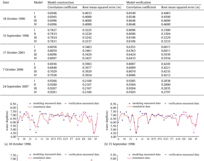
Table 4. Although the correlation coefficients for the model construction periods were generally lower than those for the model verification period, the root mean squared errors for the model construction periods were consistently smaller. The higher correlation coefficients for the model verification period are because of the fewer verification sample points. Overall, all four models had a comparable performance while Model IV (Fig. 3) was superior to the other three models and thus selected as the final optimal model. The sequential performance of the final optimal model (i.e., Model IV) was 24 September 2007, 15 September 1998, 7 October 2006, 18 October 1990, and 17 October 2001, consistent with correlation coefficient inTable 3.
For the five years, the final model has the following structures: (1) 18 October 1990: Z
=
4.
85 ln B1+
7.
01 ln B2+
5.
02 ln B3+
0.
85 ln B4+
1.
78 ln B6−
63.
05.
(12) (2) 15 September 1998: Z=
0.
18 ln B1−
0.
84 ln B2+
5.
82 ln B3−
2.
32 ln B4+
30.
67 ln B6−
150.
23.
(13) (3) 17 October 2001: Z=
12.
37 ln B1+
9.
06 ln B2+
2.
5 ln B3+
0.
32 ln B4+
10.
22 ln B6−
139.
44.
(14) (4) 7 October 2006: Z= −
5.
73 ln B1+
3.
56 ln B2+
5.
41 ln B3+
1.
17 ln B4+
28.
26 ln B6−
137.
92.
(15) (5) 24 September 2007: Z=
4.
5 ln B1+
2.
28 ln B2+
3.
08 ln B3−
1.
39 ln B4+
11.
02 ln B6−
81.
76.
(16)Table 4
Performance statistics of the final model.
Date Model Model construction Model verification
Correlation coefficient Root mean squared error (m) Correlation coefficient Root mean squared error (m)
18 October 1990 I 0.6946 0.4033 0.8549 0.4483 II 0.6945 0.4000 0.8548 0.4500 III 0.6996 0.4000 0.8648 0.4600 IV 0.6996 0.4000 0.8648 0.4600 15 September 1998 I 0.7827 0.3225 0.8096 0.3300 II 0.7833 0.3220 0.8096 0.3304 III 0.7824 0.3242 0.8106 0.3229 IV 0.7831 0.3237 0.8106 0.3233 17 October 2001 I 0.8058 0.3463 0.6355 0.6017 II 0.8059 0.3461 0.6363 0.6011 III 0.8096 0.3429 0.6424 0.5939 IV 0.8097 0.3427 0.6433 0.5934 7 October 2006 I 0.6936 0.3983 0.8087 0.4245 II 0.6840 0.3977 0.6009 0.4221 III 0.7029 0.3929 0.8070 0.4235 IV 0.7038 0.3924 0.8086 0.4212 24 September 2007 I 0.9266 0.2168 0.9285 0.2838 II 0.9280 0.2167 0.9304 0.2800 III 0.9267 0.2167 0.9284 0.2835 IV 0.9281 0.2166 0.9303 0.2797 4.00 4.50 5.00 5.50 6.00 6.50 7.00 7.50 8.00 8.50 6 16 21 4 11 16 D72 F52 G23 F7 A10 E8 G8 I5 water depth(m)
modeling measured data verification measured data simulation data 4.00 4.50 5.00 5.50 6.00 6.50 7.00 7.50 8.00 8.50 water depth(m) 6 16 21 4 11 16 D72 F52 G23 F7 A10 E8 G8 I5 modeling measured data verification measured data simulation data
(a) 18 October 1990. (b) 15 September 1998.
3.00 3.50 4.00 4.50 5.00 5.50 6.00 6.50 7.00 7.50 water depth(m) 6 16 21 4 11 16 D72 F52 G23 F7 A10 E8 G8 I5 modeling measured data verification measured data simulation data 1.00 1.50 2.00 2.50 3.00 3.50 4.00 4.50 5.00 5.50 water depth(m) 6 16 21 4 11 16 D72 F52 G23 F7 A10 E8 G8 I5 modeling measured data verification measured data simulation data (c) 17 October 2001. (d) 17 October 2006. 1.00 1.50 2.00 2.50 3.00 3.50 4.00 4.50 5.00 water depth(m) 6 16 21 4 11 16 D72 F52 G23 F7 A10 E8 G8 I5 modeling measured data verification measured data simulation data
(e) 24 September 2007.
Fig. 3. Plots showing the measured vs. predicted water depths by the final model (i.e., Model IV).
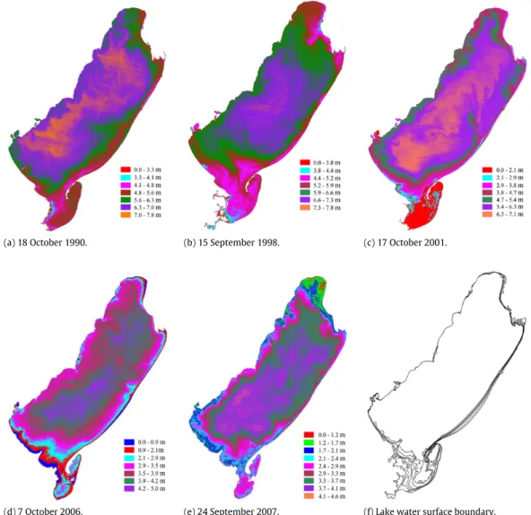
Separation of the land and water for satellite image data used masks in ENVI software, receiving image data of pure water area in Hulun Lake, then to do Band Math using Eqs.(12)–(16), acquiring the water depths distribution maps (Fig. 4(a)–(e)).
(a) 18 October 1990. (b) 15 September 1998. (c) 17 October 2001.
(d) 7 October 2006. (e) 24 September 2007. (f) Lake water surface boundary.
Fig. 4. The modeled water depths and lake water surface boundary.
Because the inflow into Hulun Lake has been decreasing since 1999, the lake level has been noticeably dropping from year to year and the cumulative decrease from 1999 to 2008 was 4 m. In accordance, the lake water surface boundary has been shrinking as well, as evidenced by the six lines inFig. 4(f) that from the outside to the inside show the lake surface extension in 1999, 2002, 2004, 2005, 2007, and 2008, respectively. The modeled water depth distributions across the lake were similar except for 15 September 1998 (Fig. 4(a)–(e)). The noticeable discrepancies occurred in the lower-left half-closed lake bays, where the constrained flow convection and distinctly different water solutes might distort the spectral characteristics. As a result, the retrieved water depths were likely to have large errors. Nevertheless, the retrieved water depths for 24 September 2007 were close to the measured values and thus can be considered as the true water depths in Hulun Lake.
The retrieved water depths for 24 September 2007 (Fig. 4(e)) were vectorized using Arc GIS 9.2, with a 0.3 m water depth interval to achieve maximum accuracy. The lake bottom elevation beneath a given water depth contour was computed as the subtraction of the lake surface elevation to the contour value. The vectorized map was stored in a shape file format.
The water–land boundaries presented by the Landsat TM/ETM
+
images taken from 1999 to 2009 were extracted using the method maximum likelihood provided by the ENVI software and stored as another shape file.These two shape themes were overlaid in Arc GIS 9.2 to generate a TIN model of the lake (Fig. 5). The TIN model is displayed with a vertical exaggeration factor of 400 because the horizontal dimensions of 90 km long and 40 km wide are a magnitude larger than the maximum water depth of 8 m.
Analysis TIN model used 3d analysis tool in Arc GIS, to calculate area and volume in different water levels (Table 5), the relationships of water level, area, and volume shown inFig. 6.
The quadratic regression equations presented inFig. 6(b) can be used to more accurately determine the volume of Hulun Lake for a given water level. As an example application, the lake surfaces for the water levels of 545, 544, 543, 542, 541, 540, 539, and 538 m were derived and are shown inFig. 7.
Fig. 5. The TIN model of the Hulun Lake bottom.
Table 5
The computed relationships of water level, area, and volume of Hulun Lake.
Water level (m) Area (km2) Volume (108m3)
545.0 2086.11 121.04 544.5 2072.65 110.64 544.0 2054.20 100.33 543.5 2031.30 90.10 543.0 1997.33 80.03 542.5 1954.74 70.15 542.0 1913.16 60.49 541.5 1844.46 51.09 541.0 1761.67 42.14 540.5 1724.21 33.43 540.0 1667.66 24.95 539.5 1546.92 16.89 539.0 1348.65 9.60 538.5 846.19 3.87 538.0 328.07 1.17 3000 2500 2000 1500 1000 500 0 area(km 2) 536 538 540 542 544 546
a
water level(m) y = 228.3x-121992 R2 = 0.747 536 538 540 542 544 546 water level(m) 140 120 100 80 60 40 20 0 volume(10 8m 3) y = 0.778 x2 - 824.896 x + 218588.883 R2 = 0.999b
Fig. 6. Plots showing (a) water level vs. area and (b) water level vs. volume.
4. Conclusion
In terms of the physiographic characteristics of lakes in cold and arid regions, this study developed a multi-band water depth retrieval model that merges the sunlight reflection band with the thermal infrared radiation band. The thermal infrared band was selected because between late autumn and early winter the water–air temperature difference is large
(a) 545 m. (b) 544 m. (c) 543 m. (d) 542 m.
(e) 541 m. (f) 540 m. (g) 539 m. (h) 538 m.
Fig. 7. 3D maps showing the derived lake surfaces of Hulun Lake at various water levels.
and the lake temperature drops more dramatically. The model merges four reflection bands 1, 2, 3 and 4, and one thermal infrared band 6. The final model took the logarithmic of these five bands as independent variables. The simulation results indicated that the model performed best for 24 September 2007 and that the model is applicable for the cold and arid region of northern China. In addition, this study derived a TIN model of the Hulun Lake bottom and regression equations of elevation, area, and volume of Hulun Lake. Compared with the existing computational method, these equations can be used to more accurately compute the lake volume for a given level. Further, this study first mapped the lake bed terrain as well as boundaries of various water levels.
Acknowledgments
We would like to thank the lakes research team at the Inner Mongolia Agricultural University for their persistent efforts in collecting/measuring the data used in this study.
The study is financially supported by the National Natural Science Foundation of China (No. 51169017, 51169011, 40901262, 50669005, 51069007); Natural Science Foundation of Inner Mongolia (No. 2012MS0612, 20091408, 20080105); International cooperation collaboration projects (2011DFA90710); Scientific and technical assistance project with develop-ing countries; Public welfare research project of Ministry of Water Resources (201101021, 201001039).
References
[1] M.C. Paul, G.B. David, Remote sensing of the coastal zone of tropical lakes using synthetic aperture radar and optical data, Journal of Great Lakes Research 29 (2) (2003) 62–75.
[2] P.C. Jennifer, L.C. Kendall, Estimating chlorophyll a concentrations from remote-sensing reflectance in optically shallow waters, Remote Sensing of Environment 101 (1) (2006) 13–24.
[3] H.D. Seelig, A. Hoehn, L.S. Stodieck, D.M. Klaus, W.W. Adams, W.J. Emery, Relations of remote sensing leaf water indices to leaf water thickness in cowpea, bean, and sugarbeet plants, Remote Sensing of Environment 112 (2) (2008) 445–455.
[4] Y.J. Wang, W.J. Dong, P.Q. Zhang, F. Yan, Progress in water depth mapping from visible remote sensing data, Marine Science Bulletin 26 (5) (2007) 92–101 (in Chinese).
[5] D.G. George, Bathymetric mapping using a Compact Airborne Spectographic Imagery (CASI), International Journal of Remote Sensing 18 (2) (1997) 2067–2071.
[6] J.C. Sandidge, R.J. Holyer, Coastal bathymetry from hyper spectral observations of water radiance, Remote Sensing of Environment 65 (1998) 341–352. [7] N.K. Tripathi, A.M. Rao, Bathymetric mapping in Kakinada Bay, India, using RS-1D LISS-III data, International Journal of Remote Sensing 23 (6) (2002)
1013–1025.
[8] R.H. Yu, Y.P. Xu, T.X. Liu, C.Y. Li, Reversing water depth in shallow lake of arid area using multi-spectral remote sensing information, Advances in Water Science 20 (1) (2009) 111–117 (in Chinese).
[10] Q.J. Tian, J.J. Wang, X.D. Du, Study on water depth extraction from remote sensing imagery in Jiangsu Coastal zone, Journal of Remote Sensing 11 (3) (2007) 373–379 (in Chinese).
[11] Y.C. Li, Z.H. Wang, Present research on monitoring drought with thermal IR remote sensing techniques in China, Agricultural Research in the Arid Areas 17 (2) (1999) 98–102.
[12] P.P. Du, W.P. Li, S.X. Sang, L.X. Wang, X.Z. Zhou, Application of 3D visualization concept layer model for coal-bed methane index system, Procedia Earth and Planetary Science 1 (1) (2009) 977–981.
[13] A.H. Mohamed, A.N. Muhammad, H.T. Yu, K. Hyoungkwan, Integrating 3D visualization and simulation for tower crane operations on construction sites, Automation in Construction 15 (5) (2006) 554–562.
[14] G. Tassilo, D. Jürgen, Abstract representations for interactive visualization of virtual 3D city models, Computers, Environment and Urban Systems 33 (5) (2009) 375–387.
[15] H.Y. Zhao, L.J. Wu, W.J. Hao, Influences of climate change to ecological and environmental evolvement in the Hulun Lake wetland and its surrounding areas, Acta Ecologica Sinica 28 (3) (2008) 1064–1071 (in Chinese).
[16] C. Li, W. Ma, X.X. Shi, W.G. Liao, Reconstruction of the hydrology series and simulation of salinity in Lake Hulun, Journal of Lake Sciences 18 (1) (2006) 13–20 (in Chinese).
[17] S.H. Wang, H.W. Liang, Y.S. Yang, Hulun wetland water environmental management measures, Inner Mongolia Water Resources 35–36 (1) (2006) 41 (in Chinese).
[18] W.B. Yan, H.H. Zhang, C.D. Zhang, Hulun lake nature reserve wetland habitats protection, Territory & Natural Resources Study (2) (2006) 47–48 (in Chinese).
[19] G.X. Yu, W.H. Wang, Y. Ma, J. Ma, The impact of grassland ecological environment by Hulunbeier wetland, Inner Mongolia Water Resources (2) (2006) 49–50 (in Chinese).
[20] H.Y. Zhao, C.C. Li, H.H. Zhao, H.C. Tian, Q.W. Song, Z.Q. Kou, The climate change and its effect on the water environment in the Hulun Lake wetland, Journal of Glaciology and Geocryology 29 (5) (2007) 795–801 (in Chinese).
[21] F.J. Tanis, H.J. Byrne, Optimization of multispectral sensors for bathymetry applications, in: Proceeding of 19th International Symposium on Remote Sensing of Environment, Ann Arbor, Michigan, 1985, pp. 865–874.
[22] J. Wei, L.C. Daniel, C.K. William, Satellite remote bathymetry:a new mechanism for modeling, Photogrammetric Engineering and Remote Sensing 58 (5) (1992) 545–549.
[23] P.C. Chu, J.C. Gascard, Deep convection and deep water formation in the oceans, in: Proceedings of the International Monterey Colloquium on Deep Convection and Deep Water Formation in the Oceans, 1991, pp. 1–382.