A parsimonious bootstrap method to model natural inflow energy series

(1)

Research Article

A Parsimonious Bootstrap Method to Model

Natural Inflow Energy Series

Fernando Luiz Cyrino Oliveira,

1

Pedro Guilherme Costa Ferreira,

2

and Reinaldo Castro Souza

3

1_{Department of Industrial Engineering, Pontifical Catholic University of Rio de Janeiro (PUC-Rio), Rua Marquˆes de S˜ao Vicente 225,}

G´avea, 22451-900 Rio de Janeiro, RJ, Brazil

2_{Brazilian Institute of Economics (IBRE-FGV), Rua Bar˜ao de Itambi 60, Botafogo, 22231-000 Rio de Janeiro, RJ, Brazil} 3_{Department of Electrical Engineering and Postgraduate Metrology for Quality and Innovation Programme,}

Pontifical Catholic University of Rio de Janeiro (PUC-Rio), Rua Marquês de São Vicente 225, Gávea, 22451-900 Rio de Janeiro, RJ, Brazil

Correspondence should be addressed to Fernando Luiz Cyrino Oliveira; [email protected] Received 19 June 2013; Revised 22 September 2013; Accepted 23 September 2013; Published 12 January 2014 Academic Editor: Youqing Wang

Copyright © 2014 Fernando Luiz Cyrino Oliveira et al. This is an open access article distributed under the Creative Commons Attribution License, which permits unrestricted use, distribution, and reproduction in any medium, provided the original work is properly cited.

The Brazilian energy generation and transmission system is quite peculiar in its dimension and characteristics. As such, it can be considered unique in the world. It is a high dimension hydrothermal system with huge participation of hydro plants. Such strong dependency on hydrological regimes implies uncertainties related to the energetic planning, requiring adequate modeling of the hydrological time series. This is carried out via stochastic simulations of monthly inflow series using the family of Periodic Autoregressive models, PAR(p), one for each period (month) of the year. In this paper it is shown the problems in fitting these models by the current system, particularly the identification of the autoregressive order “p” and the corresponding parameter estimation. It is followed by a proposal of a new approach to set both the model order and the parameters estimation of the PAR(p) models, using a nonparametric computational technique, known as Bootstrap. This technique allows the estimation of reliable confidence intervals for the model parameters. The obtained results using the Parsimonious Bootstrap Method of Moments (PBMOM) produced not only more parsimonious model orders but also adherent stochastic scenarios and, in the long range, lead to a better use of water resources in the energy operation planning.

1. Introduction

The Brazilian electrical energy production and transmission system is unique in the world, due to its continental dimen-sion and the strong participation of hydro plants (about 80% of the energy produced in the country comes from hydro plants with various owners). The national grid, also known as National Interconnected System (NIS from now on) embodies generation utilities of the following geographical regions: Southeast/Midwest, South, Northeast, and North. Only 3.4% of the generated energy in Brazil is outside the pool of the NIS; they are formed by isolated generators located, mainly, in the Amazonas region [1].

It is well known that generation systems with strong hydro share are highly dependent on the hydrological regimes. Therefore, the energy operational planning consists of deter-mining what would be the optimal amount of hydro and thermal generation for the planning horizon, that meets the projected demand and takes into account the constraints of the generation plants as well as the electrical constraints of the system [2].

As a consequence of this strong hydrological dependence, the uncertainty associated with the energy planning in Brazil requires the use of robust and reliable stochastic modeling of the hydrological time series. Hence, the need of generating

Volume 2014, Article ID 158689, 10 pages http://dx.doi.org/10.1155/2014/158689

(2)

syntheticseries from such stochastic models is required in order to produce the optimal operating costs and, at the same time, to increase the reliability of the system as a whole [3].

The energy planning in Brazil is carried out via a chain of mathematical model sand corresponding computer pro-grams, aiming at producing the optimal operation and expan-sion programs [4].

The medium range operation computer program used in the country is the so-called NEWAVE. This software produces for each month of the planning horizon (that may vary from 5 to 10 years, on a monthly basis) the optimal share of hydro and thermal resources that minimize the expected operational costs of the system. The hydro plants are represented in an aggregate manner and the estimation of the optimal opera-tional policy is carried out via a Stochastic Dynamic Dual Programming (SDDP from now on) [5].

To produce the optimal policy, NEWAVE considers a range of scenarios of energy inflows, all of them obtained by stochastic simulations having as the base models the Periodic Autoregressive structure, PAR(𝑝) models, one for each month of the year. The problem formulation is based on equivalent energy systems, that is, the four geographical sub-systems that constitute the NIS. In this approach, the hydro logical series are transformed into Natural Inflow Energy (NIE, for short) [6].

This way, the stochastic models employed to generate hydrological scenarios to be used by NEWAVE should pre-serve, as close as possible, the main features of the historical records, in order to guarantee that the produced optimal policy is reliable and satisfactory. In this paper, it is shown that the current approach to set the order and the parameters estimates of the PAR(𝑝) structures is, somehow, limited and may be improved. Indeed, the existing approach tends to identify less parsimonious AR structures and the correspond-ing parameters are estimated by the classical method of moments. The proposed improvement described in this paper uses a nonparametric technique, known as Bootstrap, which allows, among other facilities, the estimation of more reliable confidence intervals for the model parameters. The dataset used in this paper corresponds to four monthly NIE time series related to the four regions of the country (subsystems Southeast/Midwest, South, Northeast, and North), covering the period ranging from January 1931 to December 2010.

The remaining part of the paper is organized as follows. Section2presents a short overview of the existing approaches to model NIE series, including the current approach used in the Brazilian Electrical System (BES), which is, in a sense, the main criticism of the paper. It is then followed by Section3

where the proposed use of Bootstrap as an improvement tool to the existing model is thoroughly described. Finally, in the last section, the main results are presented and discussed, followed by suggestions for future researches on the subject.

2. Modeling NIE Series: A Review including

the Model in Current Use in Brazil

According to [7], the time series models applied to hydro-logical series are an important tool for the planning and

the operation of hydrothermal systems. There are a great number of papers in the specialized literature dealing with this problem for all possible types of time series observations, that is, yearly, monthly, weekly, daily, and so forth.

Among the models cited in the literature, the following are the most used: (i) Autoregressive Moving Average ARMA (𝑝, 𝑞); (ii) Pure Autoregressive AR(𝑝); (iii) Multivariate Autoregressive Moving Average MARMA(𝑝, 𝑞); (iv) Periodic ARMA(𝑝, 𝑞), (v) Periodic Autoregressive PAR(𝑝); (vi) Autoregressive Fractional Integrated Moving Average ARFIMA(𝑝, 𝑑, 𝑞); (vii) Gamma Autoregressive GAR(𝑝); (viii) Periodic Additive Autoregressive Gamma PAGAR(𝑝); (ix) Periodic Multiplicative Autoregressive Gamma PMGAR (𝑝); (x) Periodic Autoregressive Gamma PGAR(𝑝).

Concerning the use of the Box & Jenkins family of mod-els, in particular the AR structures, they can be considered as the pioneers to model hydrological series. Indeed [8] pro-posed an AR(1) to model inflows and [9] used a similar struc-ture to model monthly rainfall in Australian rivers covering the period from 1859 to 1952.

After these pioneer proposals, the following works on the area were related to improvements in their applications to hydrology problems as, for instance, in the models identifica-tion structure and parameters estimaidentifica-tions. Some important papers using AR(𝑝) and ARMA(𝑝, 𝑞) structures to model daily, monthly, and yearly hydrological series were published, such as [7, 10–16]. In the case of the two contributions by Beard mentioned above, it is addressed the question related to the inflow simulations for a particular inflow station and the extension of this result to more than one inflow station that may have a correlation structure among them.

More recently, [17] uses the AR(𝑝) and ARMA(𝑝, 𝑞)

structures to model the average monthly inflows of Goksu river, located in the Southern region of Turkey. The inter-esting aspect dealt by the author is the use of three possible ways to arrive at the model structure identification: via the Autocorrelation Function, Minimum Residual Variance, and the Akaike Information Criterion. Such analysis showed that it should be considered more than one approach to select the model order, differently of what is used in the BES that uses only one structural identification method.

Concerning the periodic class of models, the emphasis has been put on the PAR(𝑝) and PARMA(𝑝, 𝑞) structures. The PAR(𝑝) structure fits a single AR(𝑝) to each period of the series and, similarly, a PARMA(𝑝, 𝑞) structure fits an ARMA(𝑝, 𝑞) structure to each period of the series.

The extension from PAR(𝑝) into PARMA(𝑝, 𝑞) structures is not trivial, as pointed out by [18]. Besides, it is also men-tioned that the PAR(𝑝) structures have produced rather good fit to hydrological series and this would not encourage the use of more elaborated structures, such as PARMA(𝑝, 𝑞). How-ever, one can find in the literature a considerable number of papers where the adopted structure was the more elaborated PARMA(𝑝, 𝑞) as, for instance, the works by [16,19–22]. Par-ticularly, in [22] the author presents two possible ways to make the parameters estimation: via Method of Moments

(3)

(MOM) and via Maximum Likelihood (ML) and concluded that the latter produces better results than the former. On the other hand, [19] proposes an alternative way to estimate the model parameters of a PARMA(𝑝, 𝑞) model through a more parsimonious formulation and apply the approach to a monthly inflow series of Frazer river (British Columbia) and Salt river (Arizona).

In Brazil, the paper by [23] is the main reference concern-ing the production of weekly forecasts based on ARMA(𝑝, 𝑞) models, considering periodic and nonperiodic parameters. They use the software PREVIVAZ [24], developed by CEPEL (Brazilian Electrical Research Center) [25] and used by ONS, the Brazilian National System Operator [1], on the nationwide operation planning.

The model used in the BES to produce the NIE scenar-ios is the Periodic Autoregressive PAR(𝑝) structure. These scenarios are used in a SDDP, that produces the Cost to Go Functions [26,27]. As a result of this approach adopted officially in Brazil, a large number of papers have been devoted to the subject, discussing and proposing alternatives to improve this statistical procedure.

Although the use of PAR(𝑝) models has been widely used in Brazil, it is important to bear in mind that they were first proposed by [8] and have been discussed ever since in the international literature; see, for instance [28,29], that have made substantial contributions to the implementation of such models. Also it is important to mention the contributions of other authors on the discussion concerning the best way to estimate the model parameters (Method of Moment, Max-imum Likelihood, and Bayesian Inference Methods, among others) [16,22,30].

Therefore, this paper aims to propose methodological advances in the PAR(𝑝) model regarding the structure iden-tification and the model parameters estimation.

2.1. The PAR(𝑝) Model. Assuming that a time series is

com-posed of𝑛 years and 𝑠 seasonal periods of observations (in this work,𝑠 = 12 months) and that 𝑌_𝑟,𝑚is a realization of this series in year𝑟 and month 𝑚 (𝑟 = 1, 2, . . . 𝑛; 𝑚 = 1, 2, . . . , 𝑠), the Periodic Autoregressive model, PAR(𝑝), where 𝑝 is the model order (𝑝 = 𝑝₁, 𝑝₂, . . . , 𝑝_𝑚), obtained by assuming a simple AR structure for each seasonal period. The analytical expression for the PAR(𝑝) model is given by

𝑌_𝑚,𝑟− 𝜇_𝑚=∑𝑝𝑚

𝑖=1

𝜙𝑚_𝑖 (𝑌_{𝑚−𝑖,𝑟}− 𝜇_𝑚−𝑖) + 𝑎_𝑚. (1) 𝜇𝑚: expected mean for seasonal period𝑚.

𝜑𝑚

𝑖 :𝑖th autoregressive coefficient for seasonal period

𝑚.

𝑎_𝑚: independent noise series with zero mean and variance𝜎_𝑎2

𝑚for seasonal period𝑚.

Denoting𝜌_𝑘𝑚as the correlation between𝑌_𝑚,𝑟and𝑌_{𝑚−𝑘,𝑟}, and considering that (1) is an autoregressive model of the Box & Jenkins family, the parametric estimation can be conducted

by solving the Yule-Walker system [31]. For any period𝑚 we have [ [ [ [ [ [ [ [ [ [ 1 𝜌₁𝑚−1 𝜌₂𝑚−1 ⋅ ⋅ ⋅ 𝜌_𝑝𝑚−1_𝑚₋₁ 𝜌𝑚−1 1 1 𝜌1𝑚−2 ⋅ ⋅ ⋅ 𝜌𝑝𝑚−2𝑚−2 𝜌𝑚−1 2 𝜌1𝑚−2 1 ⋅ ⋅ ⋅ 𝜌𝑝𝑚−3𝑚−3 .. . ... ... ⋅ ⋅ ⋅ ... 𝜌_𝑝𝑚−1_𝑚₋₁ 𝜌_𝑝𝑚−2_𝑚₋₂ 𝜌𝑚−3_𝑝_𝑚₋₃ ⋅ ⋅ ⋅ 1 ] ] ] ] ] ] ] ] ] ] [ [ [ [ [ [ [ [ [ [ 𝜙𝑚 1 𝜙₂𝑚 𝜙₃𝑚 .. . 𝜙_𝑝𝑚_𝑚 ] ] ] ] ] ] ] ] ] ] = [ [ [ [ [ [ [ [ [ [ 𝜌𝑚 1 𝜌₂𝑚 𝜌₃𝑚 .. . 𝜌_𝑝𝑚_𝑚 ] ] ] ] ] ] ] ] ] ] . (2)

Denoting by 𝜙𝑚_𝑘𝑗 the 𝑗th autoregressive parameter of a process of order𝑘, 𝜙𝑚_𝑘𝑗 is the last parameter in this process. The Yule-Walker equations to each period𝑚 can be rewritten as follows: [ [ [ [ [ [ [ [ 1 𝜌₁𝑚−1 𝜌₂𝑚−1 ⋅ ⋅ ⋅ 𝜌_𝑘−1𝑚−1 𝜌𝑚−1 1 1 𝜌1𝑚−2 ⋅ ⋅ ⋅ 𝜌𝑘−2𝑚−2 𝜌𝑚−1 2 𝜌1𝑚−2 1 ⋅ ⋅ ⋅ 𝜌𝑘−3𝑚−3 .. . ... ... ⋅ ⋅ ⋅ ... 𝜌𝑚−1 𝑘−1 𝜌𝑘−2𝑚−2 𝜌𝑘−3𝑚−3 ⋅ ⋅ ⋅ 1 ] ] ] ] ] ] ] ] [ [ [ [ [ [ [ 𝜙𝑚 𝑘1 𝜙𝑚 𝑘2 𝜙𝑚 𝑘3 .. . 𝜙_𝑘𝑘𝑚 ] ] ] ] ] ] ] = [ [ [ [ [ [ [ 𝜌𝑚 1 𝜌𝑚 𝑘2 𝜌𝑚 𝑘3 .. . 𝜌_𝑘𝑘𝑚 ] ] ] ] ] ] ] . (3)

If the model orders were previously known, the param-eters could be obtained directly by solving the equation system (3). However, as one has to first identify the order of the model, the system (3) can be solved sequentially for each value of 𝑝_𝑚, obtaining the values for the parameters 𝜙𝑚

𝑝𝑚,1⋅ ⋅ ⋅ 𝜙

𝑚

𝑝𝑚,𝑝𝑚for each model order𝑝𝑚.

At this stage, it is important to discuss some questions regarding the model identification and parameters estima-tion. Concerning the identification of the model order, it is usually used the 95% confidence interval for𝜙𝑚_𝑘,𝑘given by the asymptotic result1.96/𝑁, where 𝑁 is the number of years of the time series. Such asymptotic interval was proposed by [32,

33]. In [34], the authors defined a Quasi White Noise process for series with this asymptotic approximation. This study was further developed by [35] for Periodic Autoregressive structures.

In practical terms, there are various ways to identify the Box & Jenkins model structure. One possible way consists of incrementing the value of𝑝_𝑚, starting from 1 until a value “𝑘+1,” for which the parameter 𝜙𝑚_{𝑘+1,𝑘+1}is no more significant. In this case, the last value of𝑝_𝑚for which𝜙𝑚_𝑝

𝑚,𝑝𝑚is significant

will be the model order; that is, 𝑝_𝑚 = 𝑘. The model parameters become𝜙_𝑘,1𝑚 ⋅ ⋅ ⋅ 𝜙_𝑘,𝑘𝑚. This criterion will be referred to here as “left to right” identification procedure (LR from now on).

The second possibility, that is, “right to left” identification procedure (RL from now on), as opposed to what happens with the LR procedure is such that the order of the model is defined as the value𝑘∗ such that, for all𝑘 > 𝑘∗, 𝜙𝑚_𝑘𝑘 is not significant. As an example, if the Partial Autocorrelation Function (PACF) shows that the lag 6 is significant and for all lags greater than 6 is not significant, the identified order will be 6, even if intermediate values for the parameters𝜙𝑚_𝑘𝑘 are nonsignificant. In actual fact, this is the way the model orders are identified in the current BES implemented in the NEWAVE computer system.

(4)

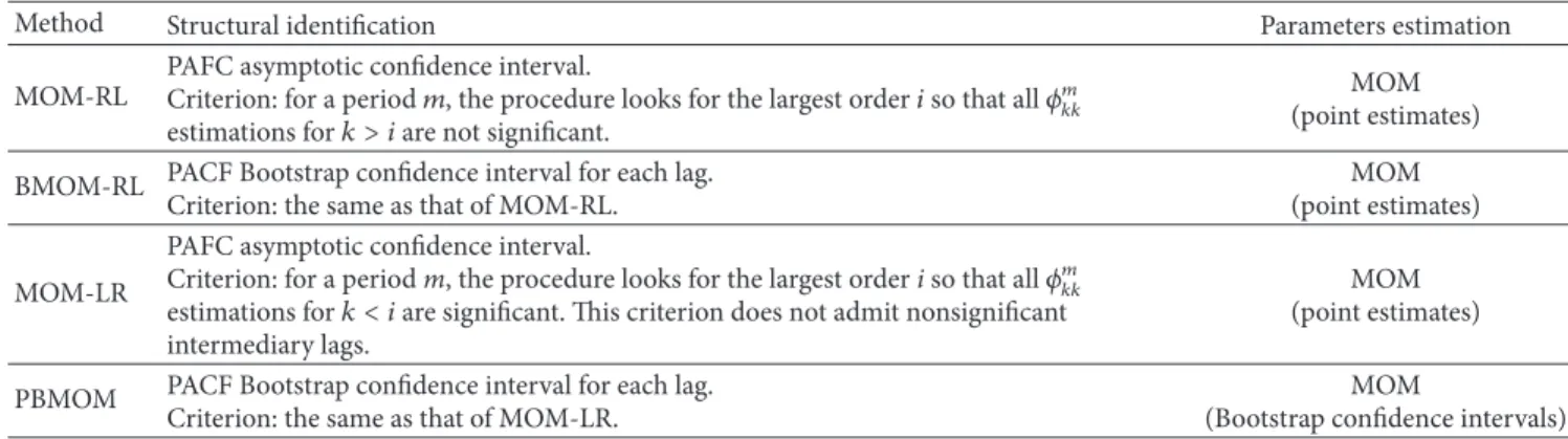
Table 1: Methods tested.

Method Structural identification Parameters estimation

MOM-RL

PAFC asymptotic confidence interval.

Criterion: for a period𝑚, the procedure looks for the largest order 𝑖 so that all 𝜙_𝑘𝑘𝑚

estimations for𝑘 > 𝑖 are not significant.

MOM (point estimates)

BMOM-RL PACF Bootstrap confidence interval for each lag.

Criterion: the same as that of MOM-RL.

MOM (point estimates) MOM-LR

PAFC asymptotic confidence interval.

Criterion: for a period m, the procedure looks for the largest order i so that all𝜙_𝑘𝑘𝑚

estimations for𝑘 < 𝑖 are significant. This criterion does not admit nonsignificant

intermediary lags.

MOM (point estimates)

PBMOM PACF Bootstrap confidence interval for each lag.

Criterion: the same as that of MOM-LR.

MOM

(Bootstrap confidence intervals)

A third way to identify the PAR(𝑝) model order was proposed recently by [35]. The authors use the resampling technique known as Bootstrap to arrive at the model order identification. It was observed that the proposed Bootstrap based approach produces results very close to that of the LR method.

Another possibility, mentioned in the appropriate litera-ture, is the minimization of some information criteria to iden-tify the model order. The most cited criteria are the Akaike Information Criterion [36] and Schwarrz Criterion [37]. The advantage of this approach is the equilibrium between the fitted model and the model parameter parsimony. In the spe-cific case of using these criteria for time series, the estimated parameters of any model will not be used if they do not con-tribute to the good fitting of the model to the series. Accord-ing to the recent literature, this is the most adequate structural identification procedure of the Box & Jenkins models; see [38]. In [39], it is emphasized the importance of this proce-dure for periodic models.

Finally, with respect to the parameters estimation, it is worth mentioning that the technique proposed in this paper is somehow similar to the one adopted in the BES; that is, it used the Method of Moments (MOM), where the sampling moments are equated to the theoretical moments obtained directly from the model analytical specification.

Once the model structure has been identified, the next step consists of obtaining estimates for the model parameters. The recommended approach to obtain these estimates is the Maximum Likelihood (ML) method. In the case of pure AR structures, like PAR(𝑝), one can also use the Method of Moment estimate procedure, as it produces similar results to ML estimation, [29].

Having the model identified and the parameters esti-mated, the next step consists of the application of a set of goodness of fit tests to check if the model has produced resid-uals that resemble a white noise process, as well as check on possible underfitting or overfitting of the model structure.

As mentioned in the introductory section, the goal of this paper is to propose improvements in the current stochastic approach used in BES, regarding the identification and estimation phases of the PAR(𝑝) model. This way, it will be possible not only to estimate parsimonious models, as the LR identification does [39,40], but also to fit the confidence

intervals to the model parameters. As a result of that, only significant parameters will be estimated by the models. There-fore, the main objective here is to raise the discussion about this subject and propose a new way to produce confidence intervals for the parameters of the PAR(𝑝) models, as well as improve on the structural identification.

Finally, four models were tested in order to evaluate the performance of the proposed approach. For each one of them, it was carried out both parameters estimates and structural order identification using different schemes, as shown in Table1. The last one, called Parsimonious Bootstrap Method of Moments (PBMOM), is the main contribution of this paper.

3. The Bootstrap Technique

Bootstrap is a computationally intensive statistical technique that allows the evaluation of the variability of estimators based on a unique sample. The technique is recommended for problems where the conventional statistical procedures are not straight forwardly implemented. It is recommended for situations with small and/or large samples, provided the results obtained are close to those obtained via the usual asymptotic analysis in large samples.

Operationally, the technique consists of drawing with replacement the elements of a finite random sample, produc-ing the so-called Bootstrap sample of the same size of the original sample. This way one can obtain a set of Bootstrap samples, enough to generate the Bootstrap distribution of the statistics of interest. Thus, the set of Bootstrap observations corresponds to an estimate of the true sampling distribution of the statistics of interest. As shown in [41], as the original sample size tends to infinity the Bootstrap distribution of the statistics converges to the true distribution of these statistics.

Let𝑋 = (𝑥₁, 𝑥₂, . . . , 𝑥_𝑛−1, 𝑥_𝑛) be the original finite sample of size 𝑛 obtained from an unknown probability model described by its distribution function 𝐹 and 𝜃 = 𝑆(𝑋) particular statistics of interest. Denote𝑋∗_𝑖,𝑖 = 1, 2, . . . , 𝐵, as the𝑖th Bootstrap sample of size 𝑛 obtained from the original sample𝑋 by means of a drawing with replacement procedure. For each sample one can obtain the corresponding Bootstrap estimate of the statistics of interest:𝜃_𝑖∗= 𝑆(𝑋∗_𝑖).

(5)

The mean, variance, and standard error of the Bootstrap estimator of𝜃 is defined by 𝜃∗₌ ∑𝐵𝑖=1𝜃∗𝑖 𝐵 , Var(𝜃_𝑖∗) =∑ 𝐵 𝑖=1(𝜃∗𝑖 − 𝜃∗)2 𝐵 − 1 , SEboot= √Var (𝜃_𝑖∗). (4) As shown in [41],

Var(SEboot) ≅

𝐶₁ 𝑛2 +

𝐶₂

𝑛𝐵, (5)

where𝐶₁and𝐶₂are constants that depend on the population distribution 𝐹, but do not depend on 𝑛 and 𝐵. The result shown in (5) illustrates that the uncertainty of the Bootstrap estimators depends, mainly, on the original sample size, no matter how big is the number of Bootstrap samples one takes (i.e., the value of𝐵). In fact, in the present application, it was not necessary to estimate explicitly this expression.

Some of the published methods to build confidence inter-vals using Bootstrap are Nonstudentized Pivotal, Bootstrap-t, Percentile, Bias Corrected Percentile, Bias Corrected and Accelerated Percentile, Inversion, and Studentized Test-Inversion. For details, see [41–43]. In this paper, it will be used the Percentile method, which is based on the percentiles of the estimated Bootstrap distribution and is adequate for paramet-ric and nonparametparamet-ric simulations, according to [42].

Denoting by ̂𝐺 the distribution function of ̂𝜃∗, then the (1−2𝛼) percentile confidence interval is defined by the 𝛼 and the (1 − 𝛼) percentiles of ̂𝐺. Hence, the lower bound value of the interval is given by ̂𝐺−1(𝛼) while the upper bound value is ̂𝐺−1(1 − 𝛼). By considering ̂𝐺−1(𝛼) = ̂𝜃∗(𝛼), then the confi-dence interval of the Bootstrap distribution can be written as [̂𝜃_%,inf, ̂𝜃_%,sup] = [̂𝜃∗(𝛼), ̂𝜃∗(1−𝛼)] . (6) It is important to emphasize that this result is theoretical and it refers to the case where the number of samples is infinite. According to [44], on the Bootstrap case, this number is finite and is given by (𝑛 being the original sample size)

(2𝑛 − 1_{𝑛 ) .} (7) Therefore, according to the previous equation, for a sample size equal to 10, it would be possible to obtain𝐵 = 92378 Bootstrap samples. In real terms, 𝐵 should be big enough to allow the calculation of the statistics of interest. On the other hand, the Bootstrap sample size 𝐵 does not necessarily need to be obtained as a result of (7). This was the case in the present application. These statistics are ordered in ascending order and, as such, the percentiles of interests are estimated. Let ̂𝜃_𝐵∗(𝛼) and ̂𝜃_𝐵∗(1−𝛼) be the [𝛼 ∗ 100%] and [1 − 𝛼 ∗ 100%] percentiles (lower and upper bound, resp.) of the ascending ordered list of the𝐵 statistics coming from

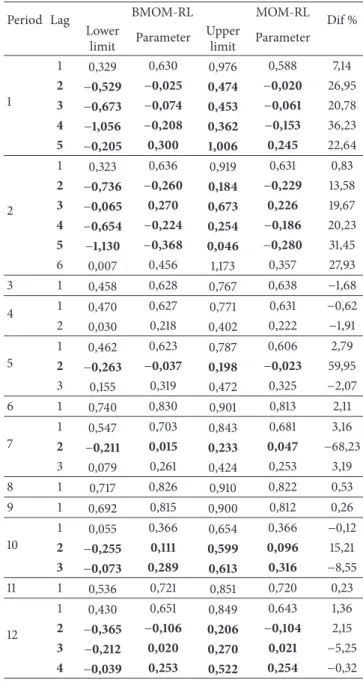
Table 2: Comparison between the parameters estimated: BMOM-RL and MOM-BMOM-RL—subsystem Southeast/Midwest.

Period Lag BMOM-RL MOM-RL Dif %

Lower limit Parameter Upper limit Parameter 1 1 0,329 0,630 0,976 0,588 7,14 2 −0,529 −0,025 0,474 −0,020 26,95 3 −0,673 −0,074 0,453 −0,061 20,78 4 −1,056 −0,208 0,362 −0,153 36,23 5 −0,205 0,300 1,006 0,245 22,64 2 1 0,323 0,636 0,919 0,631 0,83 2 −0,736 −0,260 0,184 −0,229 13,58 3 −0,065 0,270 0,673 0,226 19,67 4 −0,654 −0,224 0,254 −0,186 20,23 5 −1,130 −0,368 0,046 −0,280 31,45 6 0,007 0,456 1,173 0,357 27,93 3 1 0,458 0,628 0,767 0,638 −1,68 4 1 0,470 0,627 0,771 0,631 −0,62 2 0,030 0,218 0,402 0,222 −1,91 5 1 0,462 0,623 0,787 0,606 2,79 2 −0,263 −0,037 0,198 −0,023 59,95 3 0,155 0,319 0,472 0,325 −2,07 6 1 0,740 0,830 0,901 0,813 2,11 7 1 0,547 0,703 0,843 0,681 3,16 2 −0,211 0,015 0,233 0,047 −68,23 3 0,079 0,261 0,424 0,253 3,19 8 1 0,717 0,826 0,910 0,822 0,53 9 1 0,692 0,815 0,900 0,812 0,26 10 1 0,055 0,366 0,654 0,366 −0,12 2 −0,255 0,111 0,599 0,096 15,21 3 −0,073 0,289 0,613 0,316 −8,55 11 1 0,536 0,721 0,851 0,720 0,23 12 1 0,430 0,651 0,849 0,643 1,36 2 −0,365 −0,106 0,206 −0,104 2,15 3 −0,212 0,020 0,270 0,021 −5,25 4 −0,039 0,253 0,522 0,254 −0,32

the Bootstrap samples. For instance, in the case of𝐵 = 10.000 and𝛼 = 0.025, then lower bound value is the point in the position 250 and the upper bound value is the point in the position 9750. According to [34], this sample size is large enough to guarantee the minimum variance estimators, as shown in (5).

Hence, the approximate (1 − 2𝛼) interval is given by [̂𝜃_%,inf, ̂𝜃_%,sup] ≈ [̂𝜃∗(𝛼)_𝐵 , ̂𝜃∗(1−𝛼)_𝐵 ] . (8) The percentiles are computed from the empirical dis-tribution using the Bootstrap samples. Notwithstanding, according to [42], supported by the Central Limit Theorem, considering very large Bootstrap samples (𝐵 → ∞),

(6)

Table 3: Comparison between the parameters estimated: PBMOM and MOM-LR—subsystem Southeast/Midwest.

Period Lag PBMOM MOM-LR Dif %

Lower limit Parameter Upper limit Parameter 1 1 0,445 0,596 0,722 0,591 0,78 2 — — — — — 3 — — — — — 4 — — — — — 5 — — — — — 2 1 0,385 0,587 0,740 0,581 1,08 2 — — — — — 3 — — — — — 4 — — — — — 5 — — — — — 6 — — — — — 3 1 0,460 0,626 0,769 0,638 −1,90 4 1 0,472 0,627 0,770 0,632 −0,68 2 0,027 0,216 0,398 0,222 −2,68 5 1 0,689 0,789 0,870 0,791 −0,23 2 — — — — — 3 — — — — — 6 1 0,740 0,829 0,901 0,813 2,00 7 1 0,741 0,881 1,038 0,882 −0,06 2 — — — — — 3 — — — — — 8 1 0,716 0,826 0,909 0,822 0,50 9 1 0,693 0,814 0,903 0,812 0,19 10 1 0,440 0,658 0,837 0,668 −1,47 2 — — — — — 3 — — — — — 11 1 0,538 0,720 0,852 0,720 0,07 12 1 0,565 0,699 0,811 0,696 0,52 2 — — — — — 3 — — — — — 4 — — — — —

the Bootstrap histogram resembles a Gaussian distribution, justifying (8).

With these two intervals estimated, one can check their significance in the following way: if the zero value is within the interval[̂𝜃_%,inf, ̂𝜃_%,sup], then this parameter is nonsignif-icant and its value is zero. Otherwise, the parameter is stati-cally different from zero.

4. Results

Before presenting the results, it is important to call the attention of the reader to the correct understanding of the tables and figures containing the results of the analysis. In Tables2,4,6, and8are shown the estimated parameters and

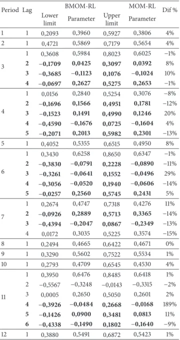
Table 4: Comparison between the parameters estimated: BMOM-RL and MOM-BMOM-RL—subsystem South.

Lower limit Parameter Upper limit Parameter 1 1 0,2093 0,3960 0,5927 0,3806 4% 2 1 0,4721 0,5869 0,7179 0,5654 4% 3 1 0,3608 0,5984 0,8023 0,6025 −1% 2 −0,1709 0,0425 0,3097 0,0392 8% 3 −0,3685 −0,1123 0,1076 −0,1024 10% 4 −0,0697 0,2627 0,5275 0,2653 −1% 4 1 0,0156 0,2840 0,5254 0,3076 −8% 2 −0,1696 0,1566 0,4951 0,1781 −12% 3 −0,1523 0,1491 0,4990 0,1246 20% 4 −0,4590 −0,1676 0,0725 −0,1604 4% 5 −0,2071 0,2013 0,5982 0,2301 −13% 5 1 0,4052 0,5355 0,6515 0,4950 8% 6 1 0,3430 0,6258 0,8650 0,6347 −1% 2 −0,3830 −0,0791 0,2228 −0,0890 −11% 3 −0,3261 −0,0641 0,1552 −0,0496 29% 4 −0,3056 −0,0520 0,1940 −0,0606 −14% 5 −0,0257 0,2560 0,5745 0,2431 5% 7 1 0,2674 0,4747 0,7318 0,4276 11% 2 −0,0926 0,2889 0,5713 0,3365 −14% 3 −0,4394 −0,2047 0,0867 −0,2349 −13% 4 0,0172 0,3035 0,5225 0,3574 −15% 8 1 0,2494 0,4665 0,6422 0,4671 0% 9 1 0,3290 0,5602 0,7522 0,5534 1% 10 1 0,2793 0,4709 0,6545 0,4530 4% 11 1 0,3950 0,6476 0,8485 0,6418 1% 2 −0,5567 −0,3248 −0,0143 −0,3315 −2% 3 0,0005 0,2650 0,5050 0,2601 2% 4 −0,3926 −0,0484 0,2668 −0,0168 189% 5 −0,1426 0,0900 0,3481 0,0813 11% 6 −0,4338 −0,1490 0,1802 −0,1640 −9% 12 1 0,3880 0,5491 0,6872 0,5423 1%

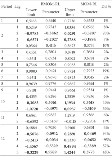
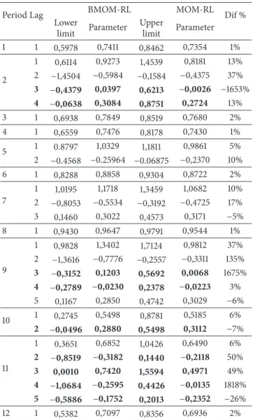
the identified orders for each one of the 12 months for both methods: BMOM-RL and MOM-RL. These procedures may result in high model orders, increasing, therefore, the risk of nonparsimonious models. The nonsignificant parameters, according to the Bootstrap significance level (that is used in the BES to generate the simulated series), are marked by bold. As a last point related to Tables2,4,6, and8, on the right hand side of them are produced the differences, expressed in percentages, between the estimated values from the BMOM-RL and the MOM-LR methods.

With respect to Tables3,5,7, and9, they show the results obtained with both PBMOM and MOM-LR. Besides produc-ing the results comproduc-ing from the two methods, there is also the comparison with the more parsimonious identification

(7)

Table 5: Comparison between the parameters estimated: PBMOM and MOM-LR—subsystem South.

Lower limit Parameter Upper limit Parameter 1 1 0,2068 0,3950 0,5896 0,3806 4% 2 1 0,4713 0,5859 0,7133 0,5654 4% 3 1 0,4563 0,6484 0,8042 0,6483 0% 2 — — — — — 3 — — — — — 4 — — — — — 4 1 0,2573 0,5004 0,7046 0,5187 −4% 2 — — — — — 3 — — — — — 4 — — — — — 5 — — — — — 5 1 0,4074 0,5355 0,6509 0,4949 8% 6 1 0,4301 0,6192 0,7740 0,6223 0% 2 — — — — — 3 — — — — — 4 — — — — — 5 — — — — — 7 1 0,5106 0,6374 0,7574 0,6126 4% 2 — — — — — 3 — — — — — 4 — — — — — 8 1 0,2442 0,4669 0,6434 0,4670 0% 9 1 0,3271 0,5573 0,7477 0,5534 1% 10 1 0,2802 0,4704 0,6523 0,4531 4% 11 1 0,4105 0,6506 0,8380 0,6467 1% 2 −0,5619 −0,3303 −0,0245 −0,3378 −2% 3 0,0112 0,2284 0,4185 0,2328 −2% 4 — — — — — 5 — — — — — 6 — — — — — 12 1 0,3905 0,5514 0,6894 0,5422 2%

method (MOM-LR) to show the importance of the reduction of the autoregressive order of the PAR(𝑝) models, specially concerning the convergence of the estimated parameters from the methods PBMOM and MOM-LR. This result, in a sense, points out the robustness of the PBMOM method.

In building the results for the BMOM-RL and PBMOM approaches,𝐵 = 10, 000 Bootstrap samples were generated. In this way, once the model order is obtained following the procedure described above, the lower and upper bounds percentiles were calculated, as well as the Bootstrap averages for each one of the lags corresponding to the autoregressive orders of the models.

Moving now to the presentation of the results by sub-systems, one can see from Table 2 that, in general, when

Table 6: Comparison between the parameters estimated: BMOM-RL and MOM-BMOM-RL—subsystem Northeast.

Lower limit Parameter Upper limit Parameter 1 1 0,5168 0,6610 0,7736 0,6533 1% 2 1 0,5249 0,7543 1,0334 0,6966 8% 2 −0,9783 −0,3862 0,0291 −0,3207 20% 3 −0,6571 −0,2027 0,2788 −0,1894 7% 4 0,0564 0,4116 0,8673 0,3731 10% 3 1 0,6551 0,7804 0,8718 0,7684 2% 4 1 0,5611 0,6934 0,8021 0,6781 2% 5 1 0,7546 0,8306 0,9083 0,8118 2% 6 1 0,9003 0,9421 0,9724 0,7923 19% 7 1 0,9511 0,9670 0,9843 0,9515 2% 8 1 0,9639 0,9776 0,9867 0,9661 1% 9 1 0,9101 0,9441 0,9661 0,9334 1% 10 1 0,4355 0,8286 1,2539 0,7836 6% 2 −0,3083 0,5061 1,1934 0,3618 40% 3 −1,0720 −0,4971 0,0937 −0,3109 60% 11 1 0,6861 0,9887 1,2919 0,9366 6% 2 −0,6892 −0,3469 −0,0115 −0,2954 17% 12 1 0,4884 0,7050 0,9160 0,6801 4% 2 −0,5076 −0,0912 0,2891 −0,0469 94% 3 −0,6113 −0,0034 0,5330 −0,0652 −95% 4 −1,4567 −0,5329 0,4884 −0,3389 57% 5 −0,3229 0,5589 1,4244 0,3773 48%

the identification is not carried out by the most parsimonious procedure, the difference between the estimated parameters by the two approaches was around 20% superior in average. Besides that, when one looks at the parameters estimated by the BMOM-RL, that allows for the estimation of confidence intervals, it can be noticed that the significant parameters obtained by the MOM-RL method (the one used in the BES) should have been classified as nonsignificant, once the value zero lies within the confidence interval. Such limitation could only be observed by the use of the Bootstrap estimation procedure.

As a counterpart to the identification criterion shown in Table2, in Table3are presented the results obtained when the identification and the estimation of the parameters are carried out using the PBMOM technique. The average difference between the estimated parameters from the PBMOM and the MOM-LR methods is less than 1%; a clear cut indication of the consistency of the method. Moreover, the recommended method, if adopted, makes the estimation of nonsignificant parameters in the models impossible.

Considering that the PBMOM produced more parsimo-nious formulations, such models were fitted and used to gen-erate scenarios, which, in a sense, reproduced the historical data for all subsystems. Mean, variance, distributional form, correlation, and negative sequence tests were performed [45].

(8)

Table 7: Comparison between the parameters estimated: PBMOM and MOM-LR—subsystem Northeast.

Lower limit Parameter Upper limit Parameter 1 1 0,5156 0,6589 0,7739 0,6532 1% 2 1 0,3713 0,5390 0,7163 0,5390 0% 2 — — — — — 3 — — — — — 4 3 1 0,6569 0,7813 0,8744 0,7683 2% 4 1 0,5608 0,6934 0,8001 0,6781 2% 5 1 0,7533 0,8301 0,9066 0,8117 2% 6 1 0,9018 0,9425 0,9720 0,9333 1% 7 1 0,9512 0,9669 0,9842 0,9514 2% 8 1 0,9642 0,9776 0,9867 0,9660 1% 9 1 0,9087 0,9439 0,9659 0,9333 1% 10 1 0,7769 0,8497 0,9031 0,8392 1% 2 — — — — — 3 — — — — — 11 1 0,6880 0,9856 1,2873 0,9365 5% 2 −0,6905 −0,3433 −0,0151 −0,2953 16% 12 1 0,4832 0,6371 0,7657 0,6233 2% 2 — — — — — 3 — — — — — 4 — — — — — 5 — — — — —

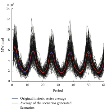
In all of them the null hypothesis of similarity with the his-torical observations was accepted at 95% level. As an example, Figure1shows that, for the Southeast/Midwest subsystem, the average of the generated scenarios and the historical series average almost coincide.

Based on the scenarios obtained by using the proposed model, the performance of these series was compared with the corresponding historical ones using Stochastic Dynamic Programming, as shown in [26]. The total expected operating costs for both sets of series were compared. This expected cost (for the whole system) is shown in Table10. It can be observed that the use of synthetic series (generated by PBMOM) allows for a cost nearly 7% lower than the one obtained with the historical series. Thus, one can state that, using this approach to produce synthetic series, it is possible to obtain more economical operation policies.

5. Final Remarks

This paper presents a new approach for the stages of structural identification and parametric estimation in order to simulate synthetic scenarios of NIE via PAR(𝑝) using the Bootstrap

Table 8: Comparison between the parameters estimated: BMOM-RL and MOM-BMOM-RL—subsystem North.

Lower limit Parameter Upper limit Parameter 1 1 0,5978 0,7411 0,8462 0,7354 1% 2 1 0,6114 0,9273 1,4539 0,8181 13% 2 −1,4504 −0,5984 −0,1584 −0,4375 37% 3 −0,4379 0,0397 0,6213 −0,0026 −1653% 4 −0,0638 0,3084 0,8751 0,2724 13% 3 1 0,6938 0,7849 0,8519 0,7680 2% 4 1 0,6559 0,7476 0,8178 0,7430 1% 5 1 0.8797 1,0329 1,1811 0,9861 5% 2 −0.4568 −0.25964 −0.06875 −0,2370 10% 6 1 0,8288 0,8858 0,9304 0,8722 2% 7 1 1,0195 1,1718 1,3459 1,0682 10% 2 −0,8053 −0,5534 −0,3192 −0,4725 17% 3 0,1460 0,3022 0,4573 0,3171 −5% 8 1 0,9430 0,9647 0,9791 0,9544 1% 9 1 0,9828 1,3402 1,7124 0,9812 37% 2 −1,3616 −0,7776 −0,2557 −0,3311 135% 3 −0,3152 0,1203 0,5692 0,0068 1675% 4 −0,2789 −0,0230 0,2378 −0,0223 3% 5 0,1167 0,2850 0,4742 0,3029 −6% 10 1 0,2745 0,5498 0,8781 0,5185 6% 2 −0,0496 0,2880 0,5498 0,3112 −7% 11 1 0,3651 0,6852 1,0426 0,6490 6% 2 −0,8519 −0,3182 0,1440 −0,2118 50% 3 0,0010 0,7420 1,5594 0,4971 49% 4 −1,0684 −0,2595 0,4426 −0,0135 1818% 5 −0,5886 −0,1752 0,2013 −0,2352 −26% 12 1 0,5382 0,7097 0,8356 0,6936 2%

technique. In particular, the Bootstrap technique was essen-tial in the estimation of the confidence interval for the PACF coefficients, leading to models far more parsimonious than the traditional asymptotic approach to set such intervals used previously. Besides this, synthetic scenarios were produced and these series were generated using the available monthly data for the four Brazilian subsystems to fit the PAR(𝑝) PBMOM structures. The obtained results using the PBMOM produced not only more parsimonious model orders but also adherent stochastic scenarios and, in average terms, lead to a better use of water resources in the energy operation planning.

As a consequence of these findings, one could state that the proposed approach in this paper is quite promising, spe-cially taking into account that it has been used for the highly complex Brazilian hydrothermal energy system. Therefore, the method could also be recommended to be used for any other large scale hydrothermal energy system.

(9)

Table 9: Comparison between the parameters estimated: PBMOM-and MOM-LR—subsystem North.

Lower limit Parameter Upper limit Parameter 1 1 0,5975 0,7403 0,8452 0,7354 1% 2 1 0,6730 0,8739 1,0839 0,8405 4% 2 −0,5967 −0,3656 −0,1490 −0,3317 10% 3 — — — — — 4 — — — — — 3 1 0,6953 0,7853 0,8530 0,7680 2% 4 1 0,6575 0,7481 0,8174 0,7430 1% 5 1 0,8797 1,0329 1,1811 0,9861 5% 2 −0,4568 −0,2596 −0,0688 −0,2370 10% 6 1 0,8313 0,8858 0,9286 0,8722 2% 7 1 1,0195 1,1718 1,3459 1,0680 10% 2 −0,8053 −0,5534 −0,3192 −0,4725 17% 3 0,1460 0,3022 0,4573 0,3171 −5% 8 1 0,9430 0,9647 0,9791 0,9544 1% 9 1 0,9721 1,3444 1,6998 1,1816 14% 2 −0,8561 −0,4723 −0,0695 −0,4080 16% 3 — — — — — 4 — — — — — 5 — — — — — 10 1 0,5242 0,7933 1,1201 0,7933 0% 2 — — — — — 11 1 0,5203 0,7075 0,8431 0,7080 0% 2 — — — — — 3 — — — — — 4 — — — — — 5 — — — — — 12 1 0,5326 0,7085 0,8351 0,6936 2%

Table 10: Expected total operating cost (R$) for the NIS.

Current model 2.1279 × 107

Proposed model: PBMOM 1.9780 × 107

Conflict of Interests

The two types of software mentioned in the paper (NEWAVE and PREVIVAZ) were developed by the Brazilian Electrical Research Center (CEPEL) to be used by the National Oper-ation System (ONS) to set the optimal dispatch of the hydrothermal Brazilian energy system. They are not commer-cial types of software and are only used by ONS and electrical energy agents. Therefore, there is no conflict of interests by any of the three authors of this paper; that is, the authors do not have direct financial relation with the commercial identities mentioned that might lead to a conflict of interests.

0 10 20 30 40 50 60 Period MW med 0 2 4 6 8 10 12 14×10 4

Original historic series average Average of the scenarios generated Scenarios

Figure 1: Average of the scenarios (red line) and historic average (blue line) for the Southeast/Midwest subsystem.

Acknowledgments

The authors would like to thank the R&D program of the Brazilian Electricity Regulatory Agency (ANEEL) for the financial support.

References

[1] ONS, 2012,http://www.ons.org.br/home/.

[2] M. V. F. Pereira, “Optimal stochastic operations scheduling of large hydroelectric systems,” International Journal of Electric

Power and Energy Systems, vol. 11, no. 3, pp. 161–169, 1989.

[3] M. V. F. Pereira, N. Campod´onico, and R. Kelman, “Long-term hydro scheduling based on sthocastic models,” in International

Conference on Electrical Power Systems Operation and Manage-ment, (EPSOM’1998), 1998.

[4] P. G. C. Ferreira, A estocasticidade associada ao setor el´etrico

brasileiro e uma nova abordagem para a geração de afluências via modelos periódicos gama [Tese de Doutorado], PUC-Rio, 2013.

[5] A. L. M. Marcato, Representac¸˜ao h´ıbrida de sistemas

equiva-lentes e individualizados para o planejamento da operação a médio prazo de sistemas de potência de grande porte [Tese de Doutorado], PUC-Rio, 2013.

[6] L. A. Terry, M. V. F. Pereira, T. A. A. Neto, L. F. C. A. Silva, and P. R. H. Sales, “Coordinating the energy generation of the Brazilian national hydrothermal electrical generating system,”

Interfaces, vol. 16, article 1, pp. 16–38, 1986.

[7] J. D. Salas and J. T. B. Obeysekera, “ARMA model identification of hydrologic time series,” Water Resources Research, vol. 18, no. 4, pp. 1011–1021, 1982.

[8] H. A. Thomas and M. B. Fiering, “Mathematical synthesis of streamflow sequences for the analysis of river basins by simula-tion,” Design of Water Resource Systems, pp. 459–463, 1962. [9] E. J. Hannan, “A test for singularities in Sydney rainfall,”

(10)

[10] L. R. Beard, “Use of interrelated records to simulate streamflow,”

Journal of Hydrology, vol. 104, pp. 13–22, 1965.

[11] L. R. Beard, “Hydrologic Simulation in water yield analysis,” Hydrology Engineering Center. US Army Corps of Engineers, 1967.

[12] J. R. Stedinger and M. R. Taylor, “Synthetic streamflow gen-eration: model verification and validation,” Water Resource

Research, vol. 18, no. 4, pp. 909–918, 1982.

[13] J. R. Stedinger, D. P. Lettenmaier, and R. M. Vogel, “Multisite ARMA(1, 1) and disaggregation models for annual streamflow generation,” Water Resources Research, vol. 21, no. 4, pp. 497– 509, 1985.

[14] N. C. Matalas, “Mathematical assessment of synthetic hydrol-ogy,” Water Resource Research, vol. 3, no. 4, pp. 937–947, 1967. [15] R. Srikanthan and T. A. Mcmahon, “A review of lag-one Markov

models for generation of annual flows,” Journal of Hydrology, vol. 37, no. 1-2, pp. 1–12, 1978.

[16] J. D. Salas, D. C. Boes, and R. A. Smith, “Estimation of ARMA models with seasonal parameters,” Water Resources Research, vol. 18, no. 4, pp. 1006–1010, 1982.

[17] U. G. Bacanli, “Stochastic modeling of monthly Streamflow data,” in Proceeding of the 5th International Scientific Conference

on Water, Climate and Environment (BALWOIS), Ohrid,

Repub-lic of Macedonia, 2012.

[18] P. F. Rasmussen, D. S. Jose, F. Laura, R. Jean-Claude, and B. Bernard, “Estimation and validation of contemporaneous PARMA models for streaflow simulation,” Water Resources

Research, vol. 32, no. 10, pp. 3151–3160.

[19] Y. G. Tesfaye, Seasonal time series models and their application to

the modelling of river flows [Ph.D. thesis], University of Nevada,

2005.

[20] Q. Shao and R. Lund, “Computation and characterization of autocorrelations and partial autocorrelations in periodic ARMA models,” Journal of Time Series Analysis, vol. 25, no. 3, pp. 359–372, 2004.

[21] A. V. Vecchia, “Maximum likelihood estimation for periodic autorregressive moving average models,” Techmometrics, vol. 27, article 4, pp. 375–384, 1985.

[22] A. V. Vecchia, “Periodic autoregressive moving avarege (PARMA) modeling with application to water resources,”

Water Resources Bulletin, vol. 21, no. 5, pp. 721–730, 1985.

[23] M. E. P. Maceira, J. M. Dam´azio, A. O. Ghirardi, and H. M. Dantas, “Periodic ARMA models applied to weekly streamflow ferecasts,” in Proceeding of the International Conference on

Electric Power Engineering (PowerTech ’99), Budapest, Hungary,

1999.

[24] Previvaz, Manual de Previs˜ao de Vaz˜oes Semanais, 2000.

[25] CEPEL, “Centro de pesquisas de energia el´etrica,” 2011,http://

www.cepel.br/.

[26] R. C. Souza, A. L. M. Marcato, B. H. Dias, and F. L. C. Oliveira, “Optimal operation of hydrothermal systems with hydrological scenario generaton through bootstrap and periodic autorre-gressive models,” European Journal of Operational Research, vol. 222, no. 3, pp. 606–615, 2012.

[27] M. E. P. Maceira, D. D. J. Penna, and J. M. Damazio, “Geração de cenários sintéticos de energia e vazão para o planejamento da operação energética,” in 16 Simpósio Brasileiro de Recursos

H´ıdricos, November, 2005.

[28] R. H. Jones and W. M. Brelsford, “Time series with periodic structure,” Biometrika, vol. 54, pp. 403–408, 1967.

[29] K. W. Hipel and A. I. McLeod, Time Series Modelling of Water

Resources and Environmental Systems, Elsevier, Amsterdam,

The Netherlands, 1994.

[30] M. Pagano, “On periodic and multiple autoregressions,” The

Annals of Statistics, vol. 6, no. 6, pp. 1310–1317, 1978.

[31] G. E. P. Box, G. M. Jenkins, and G. C. Reinsel, Time Series

Analy-sis: Forecasting and control, Prentice Hall, Englewood Cliffs, NJ,

USA, 3rd edition, 1994.

[32] M. S. Bartlett, “On the theoretical specification and sampling properties of autocorrelated time-series,” Journal of the Royal

Statistical Society, vol. 8, pp. 27–41, 1946.

[33] M. H. Quenouille, “The joint distribution of serial correlation coefficients,” Annals of Mathematical Statistics, vol. 20, pp. 561– 571, 1949.

[34] A. C. Neto and R. C. Souza, “A bootstrap simulation study in ARMA (p, q) structures,” Journal of Forecasting, vol. 15, no. 4, pp. 343–353, 1996.

[35] F. L. C. Oliveira and R. C. Souza, “A new approach to identify the structural order of par (p) models,” Pesquisa Opracional, vol. 31, no. 3, pp. 487–498, 2011.

[36] H. Akaike, “Factor analysis and AIC,” Psychometrika, vol. 52, no. 3, pp. 317–332, 1987.

[37] G. Schwarz, “Estimating the dimension of a model,” The Annals

of Statistics, vol. 6, no. 2, pp. 461–464, 1978.

[38] H. L¨utkepohl, Introduction to Multiple time Series Analysis, Springer, Berlin, Germany, 1991.

[39] R. Lund, Q. Shao, and I. Basawa, “Parsimonious periodic time series modeling,” Australian & New Zealand Journal of Statistics, vol. 48, no. 1, pp. 33–47, 2006.

[40] F. L. C. Oliveira, Nova abordagem para geração de cenários de

afluências no planejamento da operação energética de médio prazo [Dissertação de Mestrado], PUC-Rio, 2010.

[41] B. Efron and R. J. Tibshirani, An Introduction to the Bootstrap, vol. 57 of Monographs on Statistics and Applied Probability, Chapman and Hall, New York, NY, USA, 1993.

[42] J. Carpenter and J. Bithell, “Bootstrap confidence intervals: when, which, what? A practical guide for medical statisticians,”

Statistics in Medicine, vol. 19, pp. 1141–1164, 2000.

[43] D. N. Silva, O método bootstrap e aplicações à regressão múltipla

[Dissertac¸˜ao de Mestrado], IMEEC, UNICAMP, 1995.

[44] T. E. Unny and K. Cover, “Application of computer intensive statistics to parameters uncertainy in streamflow synthesis,” in

Proceeding of the Symposia on Statistics in Honours of Professor V. W. Josni’s 70th Birthdat, 1985.

[45] F. L. C. Oliveira, Modelo de séries temporais para construção

de árvores de cenários aplicadas à otimização estocástica [Ph.D. thesis], Pontifical Catholic University of Rio de Janeiro, Rio de

(11)

Submit your manuscripts at

http://www.hindawi.com

Hindawi Publishing Corporation

http://www.hindawi.com Volume 2014

Mathematics

Journal of

Mathematical Problems in Engineering

Hindawi Publishing Corporation http://www.hindawi.com

Differential Equations

International Journal of

Volume 2014

http://www.hindawi.com Volume 2014 Hindawi Publishing Corporationhttp://www.hindawi.com Volume 2014

Mathematical PhysicsAdvances in

Complex Analysis

Journal of

Optimization

Journal of

Combinatorics

Journal of Hindawi Publishing Corporation

Function Spaces

Abstract and Applied Analysis

http://www.hindawi.com Volume 2014 International Journal of Mathematics and Mathematical Sciences

Hindawi Publishing Corporation http://www.hindawi.com Volume 2014

The Scientific

World Journal

Discrete Dynamics in Nature and Society

http://www.hindawi.com Volume 2014 Hindawi Publishing Corporation

Discrete Mathematics

Journal of

http://www.hindawi.com Volume 2014 Hindawi Publishing Corporationhttp://www.hindawi.com Volume 2014

A parsimonious bootstrap method to model natural inflow energy series

Research Article