MASTER
ACTUARIAL SCIENCE
MASTER’S FINAL WORK
INTERNSHIP REPORT
Measuring the Impact of Mortality Experience on an
Actuarial Valuation
LAURA TCHOUACHE NDAYONG
MASTER
ACTUARIAL SCIENCE
MASTER’S FINAL WORK
INTERNSHIP REPORT
Measuring the Impact of Mortality Experience on an
Actuarial Valuation
LAURA TCHOUACHE NDAYONG
SUPERVISORS
: DANIEL ROSE
ONOFRE ALVES SIM ˜
OES
Abstract
For the past decades, mortality rates were observed to decrease faster than was projected. How-ever, after 2011, it experienced a slower decrease which has been significantly highlighted since the first quarter of 2015 (CMI and SIAS (2017)). Choosing appropriate mortality assumptions have therefore become of crucial importance to institutions whose liabilities are contingent on survival, like pension schemes.
In this essay, we explored the impact of a mortality experience analysis in conjunction with a postcode mortality analysis, in setting prudent mortality assumptions, wherein we discussed the recent unusual trend in mortality improvements and the fact that for the first time we may start to see mortality assumptions weakening than strengthening. We further quantified this impact with the gain (or loss) resulting from adopting the mortality assumptions agreed at the previous valuation. In particular, we focused our analysis on the funding valuation of an existing defined benefit pension scheme and, from our analysis, proposed mortality assumptions for the current valuation. We also analysed the historical mortality rates adopted by the scheme over the last seventeen years and the progression in life-expectancies of scheme members resulting from these assumptions. With this, we were able to capture the recent trend in mortality, which suggests the scheme’s mortality assumptions reflect the actual mortality observed in the general UK population. Statistical methods were used to test the validity of the results. We made use of the Demographic Agility tool and the EuVal software from Willis Towers Watson for our analysis, and the graphics were produced using the R software package.
Keywords: Mortality, Mortality Improvements, Postcode Analysis, Morality Experience.
Resumo
Ao longo das d´ecadas mais recentes, e at´e 2011, as taxas de mortalidade diminu´ıram muito mais rapidamente do que as proje¸c˜oes existentes levavam a crer. A partir de 2011, contudo, tem-se observado que o decr´escimo, embora continue, se processa agora a um ritmo muito mais lento, um fen´omeno que a partir de 2015 se tornou um t´opico relevante para todos os interessados nas quest˜oes demogr´aficas (CMI and SIAS(2017)). Entre estes interessados est˜ao as institui¸c˜oes cujas responsabilidades s˜ao dependentes de sobrevivˆencia, como a Seguran¸ca Social, ou os respons´aveis por planos de pens˜oes, para quem a escolha de hip´oteses de mortalidade adequadas s˜ao da maior importˆancia.
Neste estudo, explora-se o impacto de se considerar a pr´opria experiˆencia de mortalidade do plano,
em conjunto com a ainda incipiente an´alise da mortalidade por c´odigo postal, na defini¸c˜ao de pressupostos prudentes de mortalidade. Procura assim ter-se em aten¸c˜ao a tendˆencia recente, e inesperada, nas melhorias da mortalidade e capturar o facto de que tais melhoramentos podem estar a atenuar-se e n˜ao a robustecer-se. Adicionalmente, procura caracterizar-se o referido im-pacto com o ganho (ou perda) resultante da ado¸c˜ao dos pressupostos de mortalidade previamente estabelecidos. Num estudo de caso, procede-se `a avalia¸c˜ao do n´ıvel de financiamento de um plano de pens˜oes de benef´ıcio definido real e, em conformidade com a an´alise realizada, apresentam-se propostas para a revis˜ao dos pressupostos em vigor. Analisam-se ainda as taxas hist´oricas de mortalidade adotadas pelo plano nos ´ultimos dezessete anos e a progress˜ao da esperan¸ca de vida dos seus membros. Com isso, consegam-se a capturar a tendˆencia recente de mortalidade, o que sugere que os pressupostos de mortalidade do plano refletem a mortalidade observada na popula¸c˜ao geral do Reino Unido. Recorreu-se a m´etodos estat´ısticos para testar a validade dos resultados. Para a realiza¸c˜ao do trabalho, foi utilizado o software EuVal e Demographic Agility da Willis Towers Watson, e os gr´aficos foram produzidos usando o pacote de software R.
Contents
Abstract i
Abbreviations and Acronyms viii
Acknowledgements ix
1 Introduction 1
1.1 Objective and Layout . . . 2
2 Preliminaries on Pension Schemes 3 2.1 Occupational pension schemes . . . 3
2.1.1 Defined contribution schemes . . . 3
2.1.2 Defined benefit schemes . . . 4
2.1.3 Defined benefit lump sum at retirement . . . 5
2.2 Funding a defined benefit scheme . . . 5
2.2.1 The Trustees . . . 5
2.2.2 The sponsoring employer . . . 6
2.2.3 The scheme actuary . . . 6
2.3 Valuation of defined benefit pension scheme liabilities . . . 7
2.3.1 Actuarial assumptions . . . 7
2.3.2 Types of Valuation . . . 8
3 Setting Mortality Assumptions 11 3.1 Choosing the standard tables: Continuous Mortality Investigation . . . 11
3.1.1 Historical CMI tables . . . 11
3.1.2 The CMI SAPS Tables . . . 12
3.2 Adjusting a standard table - Scheme Mortality Experience . . . 14
3.2.1 General mortality experience methodology . . . 14
3.3 Adjusting a base table - Postcode Analysis . . . 17
3.3.1 The Methodology . . . 17
3.4 Combining the results of the postcode analysis with scheme’s experience . . . . 19
3.4.1 Bayesian analysis of the Normal distribution with known variance . . . 19
3.4.2 Applying the results to our analysis . . . 21
3.5 Future improvements in mortality . . . 22
3.5.1 The Cohort effect . . . 23
3.5.2 Floors or Underpins . . . 24
3.5.3 The CMI core projection model . . . 24
4 Analysis of Surplus 27 4.1 Reasons for an analysis of surplus and appropriate basis to use . . . 27
4.2 Analysis of surplus due to post retirement mortality . . . 28
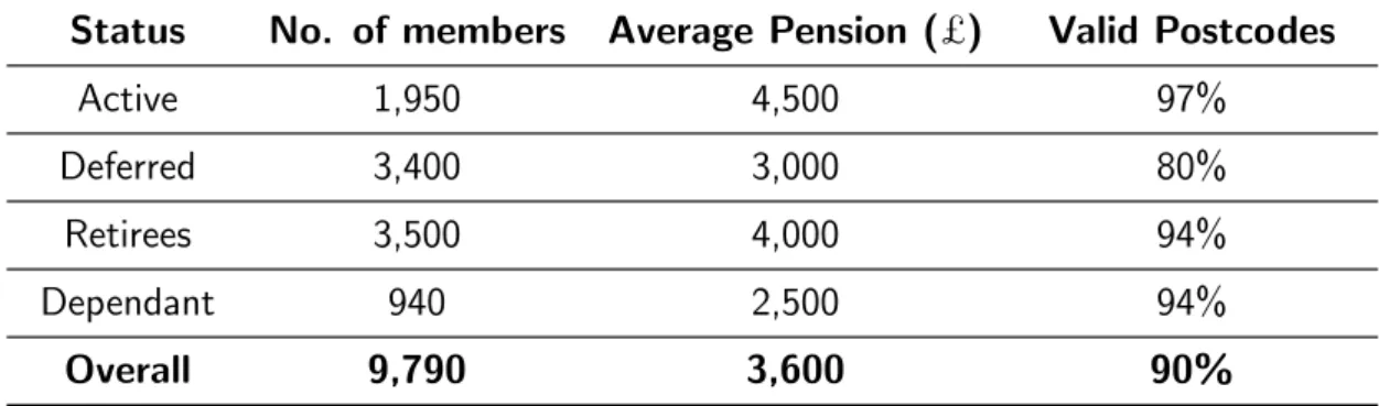
5 A Practical Example 30 5.1 Plan Information . . . 30
5.2 Fitting into the analysis of surplus . . . 31
5.2.1 The mortality assumptions . . . 31
5.2.2 Results . . . 32
5.3 Setting the mortality assumption . . . 33
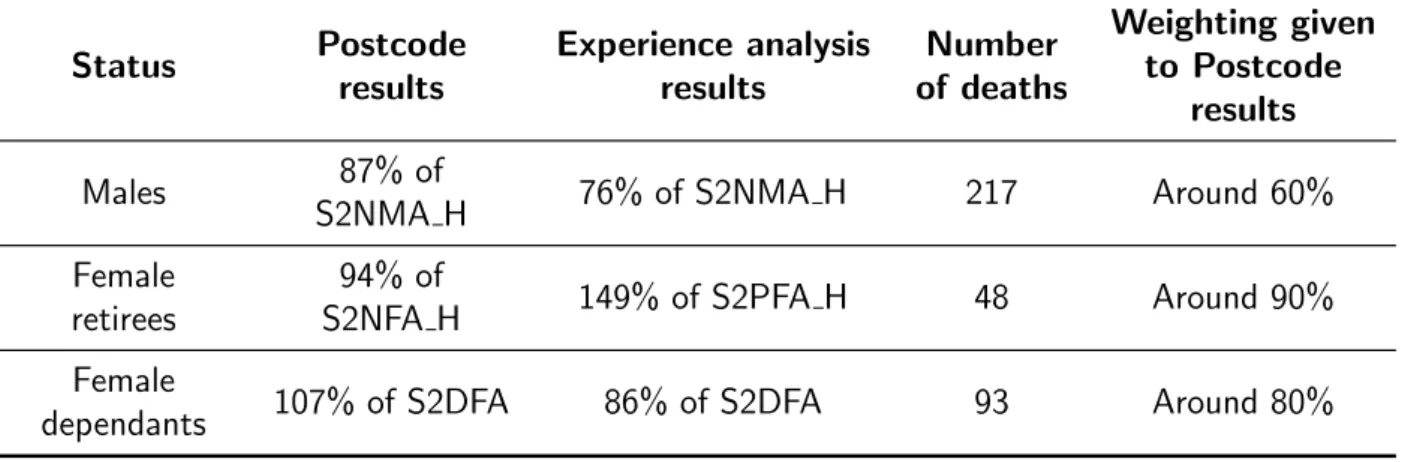
5.3.1 Actual and Expected deaths weighted by pension amount . . . 33
5.3.2 Proposed mortality assumption for the current valuation . . . 35
5.4 Historical experience analysis . . . 36
References 41
Appendix A Scheme historical mortality assumptions 42
A.1 Mortality assumptions . . . 43
Appendix B Setting mortality assumptions - credibility approach 46
List of Figures
3.1 Growth in life expectancy at birth. Source: Office of National Statistics . . . 23
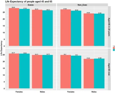
3.2 Average mortality improvement by age band. Source: CMI and SIAS(2017) . . . 26 5.1 Life expectancy using assumptions for 2014 versus 2016, for members aged 65
now and in 20 years time. . . 36
5.2 Change in life expectancy for males and females following scheme experience analysis. 37
List of Tables
3.1 Example of the SAPS S1 series. Source: (WTW,2014) . . . 13
3.2 Example of the SAPS S2 series. Source: (WTW,2014) . . . 13
3.3 Illustration of exposed to risk. . . 15
3.4 Illustration of exposed to risk contd. . . 15
5.1 Summary of Plan membership. Source: Scheme Data . . . 30
5.2 Mortality Assumptions used for Experience Analysis. Source: Scheme Experience form 31 5.3 Annuities for retirees and spouses . . . 32
5.4 A/E analysis results . . . 33
5.5 Credibility Weighting of results . . . 34
5.6 2016 Proposed 2016 mortality assumptions based on same base tables as 2014. . 35
A.1 Changes in life expectancy by year of valuation . . . 42
List of Abbreviations
Abbreviation Meaning
UK United Kingdom
CMI Continuous Mortality Investigation SIAS Staple Inn Actuarial Society PPF Pension Protection Fund DB Defined Benefit
DC Defined Contributions WTW Willis Towers Watson AoS Analysis of Surplus
ONS Office of National Statistics
SSFR Scheme Specific Funding Requirement A/E Actual to Expected
SFP Statement of Funding Principles SFO Statement of Funding Objectives SoC Statement of Contributions CPI Consumer Price Index RPI Retail Price Index MI Mortality Improvements tPR The Pensions Regulator TAS Technical Actuarial Standards IFOA Institute and Faculty of Actuaries GLM Generalized Linear Models
Acknowledgements
I give utmost gratitude to God Almighty for His constant inspiration, guidance, and protection, throughout this academic journey.
To Willis Towers Watson, for the opportunity to complete this internship under the guidance of my supervisor Daniel Rose, to whom I am grateful for his unmeasurable efforts in the accomplishment of this work.
I equally acknowledge Professor Onofre Alves Sim˜oes, for his availability, support and attention in getting this work to an acceptable academic standard.
Special thanks go to my family and friends, particularly Andree Nenkam and Hammed Fatoyinbo, for their constant motivation and moral support throughout the writing of this essay.
To everyone who gave me something to light my pathway, I say thank you.
1. Introduction
Mortality assumptions are essential in many areas of actuarial practice where the payment of benefits is contingent on survival, such as in the maintenance of private and public pension schemes, and for annuity providers. Until recent years, the actuaries’ concern was that people are living longer than they were expected to. However, in most countries, like in the United Kingdom (UK), a more prominent concern now arises regarding a different trend observed in mortality (CMI and SIAS,2017). Indeed, in the UK until 2011, mortality rates for both males and females reduced far more rapidly compared to the reduction factors implied a couple of decades ago (CMI, 2002), which translated to a rapidly increasing expectation of future lifetime. This trend has however been observed to taper as the Continuous Mortality Investigation (CMI) recorded negative results in the overall 2015 and 2016 year-on-year improvement rates, which suggests life expectancy may decrease. Nevertheless, since the CMI uses mortality data which dates back to 1975, their results show that life expectancy is still increasing, but at a slightly lower rate than in earlier CMI models. The underlying uncertainty, therefore, lies in how mortality will evolve and the future improvements in mortality rates.
Pension schemes, in particular, are exposed to this life expectancy risk, as they are in the business of funding for individuals’ retirement and often promise to make payments for the post-retirement lifetime of the individual, and after in case of a dependant contingency agreement. The impact that increasing life expectancy has on the pension plan sponsors, as well as on the UK government and the Pension Protection Fund is enormous. If the mortality improvements over time are significant, accounting for them in advance is critical. Nevertheless, setting aside too much for assumed mortality by being too conservative in the mortality assumptions may create unintended surpluses. Therefore, for pension plan Trustees, the challenge lies in correctly setting prudent mortality assumptions used to value their plan liabilities or insuring the risk.
Insuring part of the liabilities held by a scheme, by purchasing annuities, could be a possible way of mitigating the risk of fluctuating mortality rates. However, this approach induces counter-party risk and comes at a higher cost. As a result, schemes prefer to modify their mortality assumptions to reflect their current experience. The selection of mortality assumptions involves a two-step process: (i) choosing an appropriate set of base mortality tables and (ii) selecting the mortality improvement rates to be applied to these tables. In the UK, the CMI issues standard mortality tables, based on the experience of UK self-administered pension schemes. Schemes adopt and modify these standard tables to reflect their own scheme experience. The mortality improvement rates are also prescribed by the CMI and are produced each year with updated data received from the Office of National Statistics (ONS).
Section 1.1. Objective and Layout Page 2
Also, the valuation report prepared by the scheme actuary gives a comparison of how well the assumed mortality rates align to a specific scheme’s population. As part of a valuation, actuaries provide the Trustees with a gain and loss analysis (Analysis of Surplus - AoS) which reconciles the actual mortality experience of the plan to the expected experience from the last actuarial valuation. Several items fit into AoS, one of them being the post-retirement mortality experience. If the scheme consistently experiences unaccountable losses/gains because pensioner mortality is lower/higher than expected using the assumed mortality tables, this could indicate the need for a change of assumptions.
1.1
Objective and Layout
A mortality experience performed on a scheme can have two main impacts in the valuation process. In this project, our objectives are:
(i) to study how the mortality experience performed on a scheme, in conjunction with a postcode analysis, can be used in setting mortality assumptions;
(ii) and how the experience analysis fits in the AoS.
This work is a result of an internship carried out at Willis Towers Watson (WTW), and thus to make concrete our study, we consider a particular scheme XYZ1. We will show how the results got
from the scheme’s post-retirement mortality experience analysis and from the postcode analysis are aggregated to generate a set of mortality assumptions for the plan and how the experience analysis fits into the AoS. We also analyse how the mortality assumptions have changed along the years following experience analysis, and confirm the recent decreasing trend in life expectancy as recorded in (CMI and SIAS, 2017).
Most of the relevant work carried out on this topic is by the CMI. Therefore the literature review is included as references in the text from research done while completing this thesis. Other references used are internal documents available for WTW employees only.
The structure of this essay is as follows. In Chapter 2, we give a basic introduction to occupational pension schemes and the different types of valuation. We also introduce terms used throughout the text. We present, in Chapter 3, a general overview of how mortality assumptions are set considering the base tables and the mortality improvement rates. In Chapter 4, the mathematics underlying how post-retirement mortality experience fits as an item in the AoS is presented. In Chapter 5, we apply our theory to a particular scheme and give the results of our analysis. Finally, we close with some concluding remarks and propose openings for further research.
2. Preliminaries on Pension Schemes
This chapter introduces the basic notion of pension schemes which will be required throughout the text. The main references for this chapter are (Lee,1984) and (Pinsent Masons, 2011).
2.1
Occupational pension schemes
Employers set up occupational pension schemes to provide pensions for their employees. The benefits are usually paid for life, on retirement at normal retirement age of the members, but could also allow for other decrements, such as ill-health retirement, death-in-service, or withdrawals. Other benefits, usually a percentage of the total pension, could be offered such as a lump sum, or an annuity to the spouse and children (or other dependants), upon the death of the employee. There exist two primary type of occupational pension schemes, defined benefit (DB), and defined contribution (DC) schemes.
2.1.1 Defined contribution schemes
In a DC scheme, the contribution formula is defined, that is, there is a defined amount of contribution set aside yearly by the employer and (or) the employee, often as a specified percentage of the employee’s pensionable salary. This amount is saved into an account for each member. The benefit at retirement will correspond to the pension that can be bought (typically from an insurance company) with the value of the contributions made, plus any interest accrued on investments.
More formally, if the contribution is set as a percentage of pensionable salary, then
IR−x|IAx =IAx+α% Wx ¨aIR−x i,j, (2.1.1)
where
* IR is the normal retirement age;
* IR−x|IAx is the present value of the individual account for a participant aged x, at
retire-ment age;
* IAx is the value of the individual account, at age x;
* α%is the percentage of defined contribution established in the pension plan;
* Wx is the pensionable salary of the individual with age x;
Section 2.1. Occupational pension schemes Page 4
* a¨IR−x i,j is the present value of a financial annuity,iis the interest rate, and j is the salary increase rate.
The expected value of the level annual retirement benefit, BIR, for a participant with age x is
Ex[BIR] =
IR−x|IAx
aIR
(1 +i)IR−x, (2.1.2)
where aIR is expected present value of a whole life annuity at retirement age, and must be the
computed with the same actuarial assumptions used by the insurance company, to whom the risk of payment will be transferred.
In summary, we note that for a DC scheme, yearly contributions are defined, however, the benefit paid to the employee is not known for sure until retirement. The pension amount depends on the investment performance and the annuity factors available at retirement, with risk borne by the employee.
2.1.2 Defined benefit schemes
In a DB scheme, the benefit formula is defined. The pension is linked to the employee’s salary or earnings (this could be as a final salary, career average, or an average of best salaries) and years of service; thus the pension increases with an increase in wage/earnings and years of service rendered. The pension amount does not explicitly depend on any investment performance, and the employer bears all the risk.
In a final salary DB pension scheme, for example, the amount of the pension at retirement is expressed in the form:
BIR=β%x WˆIR x(IR−a), (2.1.3)
where
* BIR is the benefit at retirement age;
* β% is the accrual rate, i.e, the percentage of benefit achieved by year of service;
* (IR−a) is the number of pensionable years of service, ais the age at admission date into the scheme;
* WˆIR is the amount of projected final pensionable earnings;
Alternatively, the benefit at retirement age, BIR, could be calculated considering the entire career
average earnings. If we let Wi to be the actual earning at age i, revalued in line with a price
Section 2.2. Funding a defined benefit scheme Page 5
BIR =β%x (IR−a)x
PIR
i=a(Wi)
(IR−a) =β% x
IR
X
i=a
Wi, (2.1.4)
which is just a percentage of the cumulative wage earned during each year of service.
In a DB scheme, the employer bears all the risk (except the risk of default) and makes contributions which are expected to be sufficient to cover the benefits. The Trustees, however, may require a higher level of contribution from the sponsors, to reflect the actual scheme experience, or to cover any existing scheme deficit.
Another type of occupational pension schemes, although less frequent, is the DB lump sum at retirement.
2.1.3 Defined benefit lump sum at retirement
In this case, the employee, or dependant in case of death before retirement, receives a lump sum at retirement. The pre-retirement risk, as in the DB scheme, is borne by the employer. However, upon retirement, the members bear the risk as they are in charge of purchasing an annuity from an insurance company. Thus this is a hybrid scheme.
Given that in the company where we carried out this internship only valuations of DB schemes are performed, we will focus on DB pension schemes henceforth.
2.2
Funding a defined benefit scheme
A DB pension scheme is run by three main groups of people: the sponsoring employer, the Trustees, and the scheme actuary. Each of these is required to ensure the scheme is adequately funded. The sponsoring employer here represent the employer in charge of making contributions for the members as set by the scheme rules. The Trustees of a pension scheme are the people, acting independently from the employer, who hold the assets invested in the scheme for the benefit of the participants (Pinsent Masons, 2011). The scheme actuary, should be a fellow of the Institute and Faculty of Actuaries, and must be appointed by the Trustees to assist in carrying out its duties. At the time of writing, August 2017, useful information regarding a pension scheme funding can be found on the Pension Regulator (tPR) website http://www.thepensionsregulator. gov.uk/trustees/role-trustee.aspx.
2.2.1 The Trustees
Section 2.2. Funding a defined benefit scheme Page 6
Funding Requirement (SSFR), which replaced the minimum funding requirement in the Pensions Act 1995. One of the principal features of the SSFR is the Statutory Funding Objective (SFO). It states that a scheme must have sufficient appropriate assets to cover its technical provisions (plan’s liabilities). DB schemes need to meet the SFO which assesses their required level of funding.
Another fundamental feature of the SSFR is the statement of funding principles (SFP). The SFP is a document stating the Trustees’ policy for meeting the SFO. It includes the method and assumptions chosen by the Trustees for calculating the technical provisions and must be based on the advice of the scheme actuary. Following each valuation, the Trustees need to set up a Schedule of Contributions (SoC). The Trustees and employer must agree on the contribution rate which will be recorded on the SoC, and on a recovery plan if one is required. The SoC is to be reviewed at each subsequent valuation to reflect the current scheme experience and the changing financial conditions.
2.2.2 The sponsoring employer
The employer needs to work closely with the Trustees to ensure that the scheme meets the funding requirements. They are required to:
• Reach an agreement with the Trustee on the SFP, recovery plan and SoC.
• Provide information that the Trustee requests and reasonably needs to fulfil its duties (e.g., assessing the strength of the employer covenant). The employer covenant is the employer’s legal obligation and financial ability to support the scheme now and in the future. Depending on the strength of the covenant, Trustees will make appropriate investment and funding risk decisions.
2.2.3 The scheme actuary
The Trustees need to appoint a scheme actuary necessary to carry out actuarial valuations at least once every three years. A purpose of the valuation is to enable the actuary to advise on the contribution rate that needs to be made in future to achieve the scheme’s funding objectives. This rate must be consistent with the SFP and must meet the SFO.
Section 2.3. Valuation of defined benefit pension scheme liabilities Page 7
2.3
Valuation of defined benefit pension scheme liabilities
Financial institutions like DB pension plans, with liabilities contingent on survival, need to set aside reserves or funds to meet their payment obligations. Indeed, the scheme funding requirements of the Pension Act 2004 center on the value to be placed on a scheme’s liabilities. The amount necessary is dependent on when and for how long the benefits are to be paid for (demographic assumptions), and the amount of benefit to be paid (economic assumptions).
An actuarial valuation is an assessment which requires an actuary to advise the trustees on the choice of prudent actuarial assumptions to assess the financial health of the pension scheme (that is, a comparison of the valuation of assets and liabilities) and to determine an appropriate contribution rate to meet the cost of future benefits.
2.3.1 Actuarial assumptions
There are two main types of actuarial assumptions
1. Economic assumptions: Assumptions relating to future economic factors which will affect the funding position of the plan.
* Interest rate/discount rate: This assumption is set to discount future benefits, thus determines the plan liabilities, and should be a rational expectation of the future rate of return on the pension plan’s assets.
It is usual to have two separate assumptions for the discount rate: one for pre-retirement, and the other for post-retirement. The difference lies in the duration of the liabilities for pensioners and non-pensioners. The lower the discount rate, the more conservative the valuation of liabilities, and vice versa.
* Inflation: Benefits are often linked to price inflation (both pre and post-retirement), so projected benefits will depend on the level of inflation assumed for the future. The actuary must determine the evolution of the consumer price index (CPI) and the retail price index (RPI), and the inflation forecasts, when setting the inflation assumption.
* Salary scale: In case the benefit is dependent on the final salary on retirement (or on exit from the scheme, or on death), a salary scale assumption should be set to calculate the projected benefits. This assumption reflects expected inflation, productivity growth, merit scale, and other factors that affect wages.
Section 2.3. Valuation of defined benefit pension scheme liabilities Page 8
to meet its liability. We explore some components of demographic assumptions in more details below.
* Mortality: Analogous to a discount rate which accounts for the time value of money, the plan must assume mortality rates, both pre-retirement and post-retirement. A mortality rate is an assumed probability of dying within a year, whereas longevity refers to the future expected lifetime derived from any set of mortality rates. High mortality rates will either increase or decrease the total benefits to be paid, depending on how the value of the death benefits compares with the benefits payable should the member have survived.
Since mortality is mostly uncertain, the actuary must check the consistency of the mortality tables used in the valuation to the actual death experienced, and update the tables to reflect the plan’s mortality experience. An assumption that reflects the scheme’s experience ensures more certainty in the expected liabilities.
* Withdrawal rates: Assumptions which reflect the termination that can be expected to occur each year at each age. Schemes hope to profit from members leaving service, as the deferred benefit is only subject to price inflation and not to a salary increase. Thus, higher withdrawal rates reduce the amount of total expected liability. In case of vested rights, the law requires the transfer values to be at least equal to the cash equivalent of the deferred pension benefits accrued.
* Ill-health retirement: In case of allowance for an ill-health benefit, an assumption is needed to assess the amount to be paid. Depending on the benefit rules set on ill-health, lower assumed ill-health retirement rates might decrease the amount of expected liability. Ill-health retirement rates can be calculated partly through some analysis of national sickness rates. However, the nature of the industry and the terms of schemes vary significantly; thus a study of credible data from the scheme experience should be considered (when available) in developing the decrement table.
2.3.2 Types of Valuation
Section 2.3. Valuation of defined benefit pension scheme liabilities Page 9
Solvency Valuation: This valuation is required by the Pensions Act 2004. The solvency valu-ation is valued regarding ”discontinuance”. That is, it assumes the scheme discontinues at the valuation date (all active members are evaluated as deferred pensioners) with no further support from the company. The solvency calculation shows the cost of ‘buying out’ members’ benefits in full with an insurance company if the scheme were to be wound up.
The Trustees decide on the assumptions used for this valuation not based on the scheme’s experience, but on what is believed to be the assumptions used by the insurer. The discount rate set out is usually very low, as it often has reference to government bonds (risk-free), which results in a very high present value of the liability, when compared to that from other valuations. In summary, the solvency valuation assumes maximum prudence.
Accounting Valuation: The process of valuing the scheme’s assets for financial reporting pur-poses. The accounting valuation is valued on ”ongoing” basis, that is the scheme is assumed to be financially healthy and will continue to operate. It is required by the employer in the prepa-ration of the year-end accounts. The method used to set the assumptions is prescribed by the relevant accounting standards, which depend on where the accounts will be disclosed, but should be a ”best estimate”.
The discount rate for this valuation is set regarding ”high-quality corporate bonds”, and thus is higher compared to the discount rate used in the solvency valuation. The mortality assumptions set are usually the best estimate from the scheme experience. Accounting valuation is essential because the value of the assets on the company’s financial statement needs to be reliable. The report from this valuation allows users of the accounts, especially the shareholders, to study the financial position of the company.
Pension Protection Fund (PPF) Valuation: Schemes are required by the Pensions Regulator and the PPF to carry out, at least once in three years, a PPF valuation, according to Section 179 of the Pensions Act 2004. The purpose is to establish the level of the scheme’s assets and liabilities needed to set the PPF levy it will pay to the Pension Protection Fund (PPF (2017)). As with the solvency valuation, the PPF valuation is valued on ”discontinuance” basis.
In case of a qualifying insolvency event, and where the DB scheme meets the eligibility require-ments set by the Pension Act 2004, a valuation under Section 143 of the Act will determine whether the scheme has adequate funds to pay at least the PPF levels of compensation. This valuation should be carried out by an appointed actuary, with the valuation date set to the day before the insolvency event occurred.
com-Section 2.3. Valuation of defined benefit pension scheme liabilities Page 10
pensation (about 90% of total pension, subject to a cap, for members not yet over their normal pension age, but 100% for members who are already pensioners) and not pensions that members would receive from the plan.
Funding Valuation: This triennial valuation is required by the technical actuarial standards (Board for Actuarial Standards, 2009) and the Pensions Act 2004. We value the scheme lia-bilities on an ”ongoing” basis. The purpose of the valuation for funding purposes is to try to ensure that the plan sponsors control the costs of the scheme. If the funding position of the scheme appears unable to meet the promised benefits, the employer will have to increase the contributions; alternatively, a contribution holiday could be taken in case the funding position is higher than necessary. The assets are taken at market value, and the liabilities are valued using assumptions consistent with market conditions. The assumptions used to value the liabilities are to be determined by the scheme actuary and based on scheme-specific experience where possible.
The legislation requires Trustees to adopt assumptions which include a margin of prudence below the best estimate of mortality rates (Board for Actuarial Standards, 2009). There is no agreed definition of what prudence means; the Trustees must decide based on actuarial advice. The strength of the employer covenant is necessary for the Trustees in this valuation. If the Trustees believe that the covenant is strong, they might be willing to accept a lower level of prudence since the employer can meet any further deficit.
3. Setting Mortality Assumptions
One of the main impacts that an experience analysis can have on a valuation process is in the setting of new mortality assumptions, which reflect the scheme membership and experience, for future valuations.
Assumptions about future mortality rates play a vital role in the many actuarial calculations in the fields of life insurance and pensions. In particular, for DB pension schemes, mortality assumptions are used in projecting when, and for how long, the employers are expected to pay benefits. These assumptions help in the calculation of the pension scheme total liabilities (and thus contributions to be made by the employer to meet these), transfer values (vested rights upon withdrawal), mergers and acquisitions, and in the consolidation of the PPF.
For most schemes, the selection of a prudent mortality assumption generally involves a two-step process: (i) setting base mortality tables, which usually comprise of choosing a set of appropriate standard mortality tables (considering the average level of mortality across the scheme, and the shape of the tables), and deriving the multipliers necessary to adjust the standard tables for prudence; and (ii) applying future mortality improvement rates. In what follows, we explore ways in which the standard tables can be chosen and adjusted to reflect the scheme’s experience, and the allowance for future improvements in mortality.
3.1
Choosing the standard tables: Continuous Mortality
Investigation
The most common source of standard tables in the UK is the CMI. The Continuous Mortality Investigation Bureau was set up by the Institute and the Faculty of Actuaries in the 1920s to gather and analyse mortality data from life insurance offices and to publish the results. Since 1955, the CMI Bureau has been gathering statistics on the mortality of insured pension schemes (Wilkie (1992)).
3.1.1 Historical CMI tables
There are several pensioner’s mortality tables. The oldest tables are based on the 1967-1970 mortality experience collected from UK insurance companies. Examples include the life office pensioner male amount, PA(90)m, and the life office pensioner female amount, PA(90)f. These tables did not allow for any improvement in mortality. We also have the ”92 series”, based on the
Section 3.1. Choosing the standard tables: Continuous Mortality Investigation Page 12
experience of annuitants of UK insurance companies from 1991-1994. Examples of tables in this series include the PMA92 (male pension amounts) and the PFA92 (female pension amounts). The latest static tables were the ’00’ series, for example, the PNMA00, based on 1999-2002 experience and around 90,000 deaths, published in CMI Working Paper 22 (CMI,2006). Until recently, most pension scheme valuations were carried out based on the experience of life insurance companies.
The CMI Self-Administered Pension Scheme (SAPS) investigation collects data from actuarial consultancies, the PPF, and occupational pension schemes in respect of self-administered pension schemes (CMI, 2004). The data collected are analysed for reliability and consistency and then smoothed to create a series of tables. A proper description of the process can be found in Working paper 34 of CMI (CMI,2008a). The most significant change between the old tables and the graduated SAPS tables is the move from the initial exposed to risk to the central exposed to risk in the calculation of the exposure for the CMI rates. Due to the limitations associated with the use of initial exposed to risk calculations as pointed out in the paper CMI (2008c), the central exposed to risk is used. Thus the estimate of the crude rate is given by
µx+1 2 ≈
Dx
Ex
=mx, (3.1.1)
where Dx = deaths for age x last birthday, and Ex = exposure for age x last birthday. Simply
put age x last birthday is the curtate of the member. Since the central exposed to risk makes use of the Poisson model, an estimate for mortality rate (Alexander, C., 1998),qx is
qx = 1−e−
R1 0 µx+tdt.
3.1.2 The CMI SAPS Tables
In October 2008, the CMI published the first standard tables based on large data set relevant to most occupational pension schemes. These are called the SAPS ’S1’ series, published in CMI Working Papers 34 and 35 (CMI(2008a),CMI(2008b)), and were derived using pension scheme mortality experience between 2000 and 2006. The data collected includes about 10 million lives and around 380,000 deaths, and was collected from 350 separate pension schemes. This series comprises of 20 tables, covering a wide range of pension schemes. The tables are split by gender, lives, amounts, health status, and dependants status. The mortality rates, qx in this series apply
Section 3.1. Choosing the standard tables: Continuous Mortality Investigation Page 13
Table Explanation
S1NMA Normal health male pensioners (excluding dependants) by amount
S1NMA L Normal health Males (excluding dependants) with high pension amount, above £13,000pa (light tables)
S1NMA H Males with lower pension amount, below £1500pa (heavy tables)
S1DFA(or L) Female dependant by amounts (or lives)
Table 3.1: Example of the SAPS S1 series. Source: (WTW,2014)
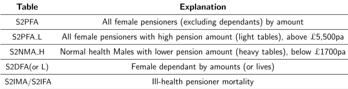
More recently, in February 2014, the CMI published the latest version of the SAPS tables - the final SAPS ‘S2’ series (comprising of 18 tables), published in CMI Working Paper 71 (CMI,2014) and based on experience between 2004 and 2011. These tables cover a wide range of pension schemes and are split like the S1 series. The Heavy, Light or All SAPS mortality tables provide users with a choice of shapes (that is, the progression of mortality rates from age to age). The range of the S2 tables is such that by adjusting with an appropriate scaling factor, it should be possible to achieve an acceptably good base mortality table for most schemes. The mortality rates, qxin this series apply from the 1 January 2007. Table 3.2 gives some examples of the ”S2”
series tables.
Table Explanation
S2PFA All female pensioners (excluding dependants) by amount
S2PFA L All female pensioners with high pension amount (light tables), above £5,500pa
S2NMA H Normal health Males with lower pension amount (heavy tables), below £1700pa
S2DFA(or L) Female dependant by amounts (or lives)
S2IMA/S2IFA Ill-health pensioner mortality
Table 3.2: Example of the SAPS S2 series. Source: (WTW,2014)
Section 3.2. Adjusting a standard table - Scheme Mortality Experience Page 14
3.2
Adjusting a standard table - Scheme Mortality
Experi-ence
According to the Regulation 5(4)(d) of the Scheme Funding Regulation , ”any change from the method or assumptions used on the last occasion on which the scheme’s technical provisions were calculated must be justified by a change of legal, demographic or economic circumstances (Parliament of the United Kingdom (2005)).” Trustees of pension schemes may thus request a mortality experience of the scheme, as one justification for changing the mortality assumptions from the last valuation.
A mortality experience examines if the mortality assumptions used in a valuation reflect the scheme’s actual experience at the time of the experience study. By this, the Trustees have a better feel of how the actual number of deaths compared to the number of expected deaths using the previously assumed mortality assumption. A scheme may decide to undertake post-retirement mortality experience (that is for the retirees and dependants) and (or) pre-retirement mortality experience (for the active and deferred members). Typically, the analysis is carried out using live and exit data from the three or six years preceding a valuation.
3.2.1 General mortality experience methodology
To carry out a mortality experience analysis, schemes undergo the following steps:
Step 1: Identify similar groups: Apart from groupings by gender and age cohorts, some schemes may choose to have the experience per other groups, say for executives, and staff members, or as a whole. These groups are justified since we expect the mortality for executive members, with a higher standard of living, and higher pension amounts, to be less than that for the general employee population.
Step 2: Calculate the amount weighted ”exposed to risk”: As earlier mentioned, the CMI SAPS tables make use of the central exposed to risk. The central exposed to risk Ec
x for a life
aged x is the time from date A to date B, where date A is the latest of
• the date of reaching age x,
• the start of the investigation (in this case, the last valuation date),
• the date of entry into the scheme,
and date B is the earliest of
Section 3.2. Adjusting a standard table - Scheme Mortality Experience Page 15
• the end of the investigation (in this case, the current valuation date),
• the date of exit (for whatever reason).
The age definition usually used is the ”age last birthday”, i.e, an individual is considered to be aged x until he/she reaches their x + 1 birthday. An illustration is given next to clarify the concept.
A mortality experience analysis covers the period 31 December 2001 to 31 December 2003. It is necessary to find the range of dates for which the lives in the following table contribute to the
Ec
34. Assume the day of entry counts in the exposure, but the day of exit does not.
Life Date of birth Date of Joining Date of exit Reason for exit
L1 25.04.69 07.08.99 30.10.03 Death
L2 30.07.68 12.09.02 -
-L3 04.09.68 22.07.03 4.10.03 Withdrawal
Table 3.3: Illustration of exposed to risk.
Applying the definition for date A and date B, it follows that:
Life Date A Date B Time in investigation L1 25.04.03 29.10.03 187 days
L2 12.09.02 29.07.68 320 days
L3 22.07.03 03.10.03 73 days
Table 3.4: Illustration of exposed to risk contd.
So for example, member Life 1 contributes to an exposure of 187/365 year for the year 2003 in age 34. For amounts exposure, the lives exposure for a particular age cell is multiplied by the (known or estimated) rate of pension applicable to that age cell. In a mortality experience, the total exposure is calculated by summing the amount of pension paid at each age.
Step 3: Divide the actual deaths by the Exposure: The actual number of deaths for each age, and in each age group is divided by the total exposure as in equation (3.1.1) to get crude rates for each age x.
Section 3.2. Adjusting a standard table - Scheme Mortality Experience Page 16
The adjustment could either be by age rating (treating members as older or younger than they are) or, more commonly, by assuming a multiplier (assuming mortality is a percentage heavier or lighter than the rates in the standard table) to reflect the scheme’s current experience analysis. So the actuary finds the multipliers needed to be applied to the best estimate tables as a margin of prudence.
The base table multiplier could result from the actual (A) to expected (E) deaths (weighted by amounts), A/E ratio. The expected deaths are calculated by multiplying the mortality rates from the assumed standard table in the last valuation, by the exposed to risk. However, it is important to note that the data used to carry out the mortality experience must be statistically credible, a notion we explain in more details in Appendix B.
Usually, at least 300 deaths are required during a three-year inter-valuation period for an experi-ence analysis data to be credible enough to adjust the standard table independently. In the case where the number of deaths is credible, then we define the A/E ratio as
A/E =
Pτ
x=α
Pmx
j=1bxjdxj
Pτ
x=a
Pmx
j=1bxjqExExjc
, (3.2.1)
where
• mx, x=α, .., τ is the number of members in the mortality experience study agedx; andα
and τ are the minimum and maximum ages, respectively, of the members included in the experience studies;
• bxj is the accrued pension for the jth member, agedx;
• dxj =
n
1,if thejthmember agedx,dies during the year
0,otherwise
o
, j = 1, ..., mx;
• qE
x is the expected mortality rate at age x using the current standard table; • Ec
xj is the central exposed to risk for the jth member, agedx.
Thus, we set the new mortality table as A/E ∗qE
x, for all ages x and this represents the ”best
Section 3.3. Adjusting a base table - Postcode Analysis Page 17
Where the scheme is too small to rely solely on its own experience for setting mortality assumptions but the number of observed deaths is not insignificant, the results of a Postcode Analysis adapted to a scheme’s experience, can be used to set new assumptions.
3.3
Adjusting a base table - Postcode Analysis
Where a scheme does not have an adequately large membership for the analysis of the scheme’s own mortality experience to be fully statistically credible, the choice of appropriate tables, in-cluding any adjustments, will need to be guided by a more extensive experience by considering of factors which are known to be correlated with observed mortality. However, many of the factors known to have the most direct influence on mortality, such as smoking habits, will not be readily available so that proxies, like postcode, will be needed.
An extensive study of census and pension scheme data show that life expectancy varies signifi-cantly between postcodes (Hume and Womersley(1985)). That is it varies from region to region, district to district, sector to sector, and unit to unit. In the UK for example, the ONS reported that the life expectancy at birth for a male in Glasgow was about 71.1 in contrast to that in Chelsea which was about 84.4, in 2011. This is about 13 years difference for people in the same county but different regions. Thus, analysis of members’ postcode can help to identify differ-ences in mortality and give a better understanding of the concentration of longevity risk within a scheme. It can also help to validate the results of other mortality investigations. This analysis can be used to adjust the standard mortality table to take into account the particular characteristics of the plan members.
Recently developed postcode models, like the Willis Towers Watson (WTW) Postcode Mortality Tool is widely used to assist assumptions setting where a scheme has insufficient experience data to determine its credible adjustment to a standard table. The overall aim of the tool is to determine a baseline mortality rate that can be adjusted for individual schemes to allow for differences in members’ characteristics, defined primarily in terms of postcodes.
In this section, we describe the method used to carry out postcode analysis and the different risks involved. The primary reference to this section is the internal document on WTW Postcode Mortality Tool (WTW, 2015).
3.3.1 The Methodology
Section 3.3. Adjusting a base table - Postcode Analysis Page 18
industries, sectors and geographical locations. The methodology is as follows:
1) Using this data, baseline mortality tables are derived by analysing the mortality observed in the entire postcode dataset.
2) The postcodes are used to generate a health and lifestyle profile for each member.
3) A statistical analysis using stepwise regression is performed to determine which factors are highly predictive of mortality. These factors then form the basis of the postcode mortality tool, and can be applied to any population of pension scheme members.
4) The number of deaths is then modelled with a GLM. Therefore, considering a given SAPS table, a mortality multiplier can be calculated to adjust the table, based on the scheme’s membership profile. The multiplier represents the expected mortality for each person com-pared to the SAPS table.
To define the GLM, we followed the steps:
- Define the distribution for the data: since the response variable is a count, we used the Poisson distribution.
- Choice of the linear predictor which is a function of the explanatory variables (age, sex, pension amount, etc): η=γ0+Pni=1γiXi,whereγ0 is the intercept, theγi are the coefficients for each
respective explanatory variable Xi, i= 1,· · ·, n.
- Choice of the link function connection the mean of the response to the linear predictor: we used the loglink, g(µ) = ln(µ).
The relationship between the response and the explanatory variables is defined through
E[D] =µ.
Given that η=g(µ) = ln(µ), we therefore have
µ=eη (3.3.1)
For a particular scheme, each member of the scheme is assigned a mortality multiplier based on their predictive factors (age, sex, pension amount, etc). The individual multipliers are used to produce summaries of average multipliers across the whole scheme.
Section 3.4. Combining the results of the postcode analysis with scheme’s experience Page 19
analysis, we can look at this information for each member of the pension plan to determine a unique socio-economic and demographic “fingerprint” for its membership. The result from the WTW Postcode Morality Tool is the best estimate of the mortality of a scheme. In order to allow for an appropriate margin of prudence for the funding valuation, the mortality ASK team in WTW set out an internal guide with necessary adjustments for any given level of prudence.1
Limitations of the Model
There are two main limitations to the model described above. Firstly, the underlying assumption in the model is that a pension scheme’s members have similar profile to the general database. However, individual schemes may have specific factors, for example, the members of a scheme may have a specific health profile (e.g., prolonged exposure to harmful chemicals) which would not be reflected in the overall population, and would result in a biased estimate of scheme’s mortality rates.
Also, for non-pensioner members, there is no allowance for members to move into ”healthier” postcode areas as they age, which means that their life expectancy may be understated.
3.4
Combining the results of the postcode analysis with
scheme’s experience
To combine the results of a postcode mortality analysis with an own-scheme experience analysis, we make use of Bayesian statistics. We assume that the postcode result is the prior with a Normal distribution, which we adjust by a Normally distributed likelihood function generated by an analysis of the scheme’s own experience. In our analysis, we assume the variance of the prior distribution (Postcode results) is known, but the mean (the multiplier to the standard table from the Postcode results) is unknown. We also treat the own-experience analysis as a new (single) observation of the mean with a corresponding known variance (WTW,2016).
3.4.1 Bayesian analysis of the Normal distribution with known variance
The material in this subsection are sourced from (Murphy, K. P., 2007).
Let X ∼N(µ, σ2), then
f(x|µ, σ2) = √ 1
2πσ2e
−(x−µ)2
2σ2 . (3.4.1)
1For the sake of ”information security” some details particular to the WTW Postcode Mortality Tool have
Section 3.4. Combining the results of the postcode analysis with scheme’s experience Page 20
If we define the precision, τ, as the reciprocal of the variance, i.eτ = σ12; then equation (3.4.1) becomes
f(x|µ, τ) =
r
τ
2πe
−τ(x−µ)2/2
. (3.4.2)
If we assume we have a set of n i.i.d normally distributed data points X where each individual point X ∼N(µ,1/τ), and µ∼N(µ0,1/τ0), then the likelihood function for our model is:
L(µ|x) = fX|µ(x|µ) = n
Y
i=1
r
τ
2πexp −τ(xi−µ)
2/2
= τ
2π
n/2
exp −1/2τ
n
X
i=1
(xi−µ)2
!
= τ
2π
n/2
exp
"
−1/2τ
n
X
i=1
(xi−x¯)2+n(¯x−µ)2
!#
,
where the last equation is obtained by applying the formula for sum of differences from the mean, and
¯
x= 1
n
n
X
i=1
xi.
The density function of the prior distribution is given by
f(µ) =
r
τ0 2πexp
−12τ0(µ−µ0)2
.
From Bayes’ theorem, we know that the posterior distribution fµ|X(µ|x) ∝L(µ|x)f(µ); so, we
have
fµ|X(µ|x) =
τ
2π
n/2
exp
"
−1/2τ
n
X
i=1
(xi−x¯)2+n(¯x−µ)2
!# r
τ0 2πexp
−1
2τ0(µ−µ0) 2
∝ exp −1
2 τ
n
X
i=1
(xi−x¯)2+n(¯x−µ)2
!
+τ0(µ−µ0)2
!!
∝ exp
−12 nτ(¯x−µ)2+τ0(µ−µ0)2
= exp −1
2(nτ +τ0)
µ− nτx¯+τ0µ0 nτ +τ0
2
+ nτ τ0
nτ +τ0(¯x−µ0)2
!
∝ exp −1
2(nτ +τ0)
µ− nτx¯+τ0µ0 nτ +τ0
2!
Section 3.4. Combining the results of the postcode analysis with scheme’s experience Page 21
In the above derivation, we eliminated the terms not involving µ, and the result approximates to a normal distribution with mean nτx¯+τ0µ0
nτ+τ0 , and precision nτ +τ0, that is
fµ|X(µ|x)∼N
nτx¯+τ0µ0
nτ +τ0
, 1 nτ +τ0
.
Now, writing this in terms of the variance, we have that fµ|X follows a normal distribution with
parameters
µ′0 =
n¯x σ2 +
µ0
σ2 0
n σ2 +σ12
0
, and σ02′ = n 1
σ2 + σ12 0
. (3.4.3)
3.4.2 Applying the results to our analysis
Following our analysis, we have n = 1, since we consider the scheme’s own-experience analysis as a single observation. Therefore, replacing the notations in equation 3.4.3 by our notations, considering the postcode results as the prior and the experience analysis result as the newly observed data,
Combined mean=
µp σ2 P + µE σ2 E 1 σ2 P + 1 σ2 E (3.4.4) and
Combined standard deviation=
1 σ2 E + 1 σ2 P
−12
, (3.4.5)
where µp is the multiplier from the postcode result;
σp is the standard deviation from the postcode result;
µE is the multiplier from the scheme’s own experience analysis;
σE is the standard deviation from the scheme’s own experience analysis.
A reasonable estimate of the standard deviation of a lives-weighted experience analysis would be:
σE =
1
√
T otal number of deaths. (3.4.6)
Section 3.5. Future improvements in mortality Page 22
Allowing for this, we can estimate the standard deviation of the postcode analysis as follows:
σP =
s
0.3
√
T otal number of deaths÷7.5%
2
+ 0.062+ 0.072+ 0.0052
Φ−1(0.95) , (3.4.7)
where the values 0.06, 0.07, and 0.005 are the reductions needed to be applied to the multiplier from the postcode result to cover respectively for model risk, parameter risk, and out of sample risk with a 95%confidence level. Model risk assumes that some schemes do not precisely fit the GLM model used, parameter risk assumes that some more variables may be predictive of mortality which the model does not include.
We can rewrite the combined multiplier given in equation (3.4.4) as a credibility weighting of both the results as follows:
Combined multiplier =
µp σ2 P + µE σ2 E 1 σ2 P + 1 σ2 E
=µE x
1 σ2 E 1 σ2 E + 1 σ2 P
+µP x
1 σ2 P 1 σ2 E + 1 σ2 P , that is
Combined multiplier =zµE+ (1−z)µP,
where z = 1 σ2 E 1 σ2 E + 1 σ2 P . (3.4.8)
3.5
Future improvements in mortality
Another basic component in setting mortality assumptions for a scheme is to allow for future mortality improvements. Mortality improvement is a measure of how mortality changes over time. Improvements to mortality vary by gender, age, period and cohort.
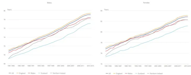
Looking at Figure 3.1, taken from the ONS, we see that the life-expectancy for both females and males, have grown along the years. Thus, it is important for mortality assumptions to incorporate an assumption for future improvement in mortality.
The models used in forecasting mortality can be classified into three main categories: process-based, explanatory and extrapolative, see Rosner et al. (2013) for a detailed comparison of each of these models.
fo-Section 3.5. Future improvements in mortality Page 23
(a) Male life expectancy at birth in the UK, and other constituent countries.
(b) Female life expectancy at birth in the UK, and other constituent countries.
Figure 3.1: Growth in life expectancy at birth. Source: Office of National Statistics
cus on the factors that are known to determine deaths. The model assumes independence among the causes of death, while in reality, the different causes of death can be interrelated. These methods are only highly useful to the extent that the process causing death is fully understood, and can be modelled mathematically.
Explanatory-based methods use econometric techniques (like regression) to predict mortality based on economic or environmental factors. These methods require the determination and prediction of a set of explanatory variables which is almost as difficult as predicting mortality directly. They are not very used.
Extrapolative methods are based on projecting historical trends of mortality into the future. Sim-ple extrapolative methods are only reliable if the conditions which led to changing mortality rates in the past continue to have a similar impact in the future. However, medical advances and im-provement in technology could invalidate the result. Extrapolative methods could be parametric methods which involve fitting a parametrized curve to the data and projecting trends in these parameters forward (for example Lee-Carter or P-spline interpolation models), or targeting meth-ods which involve assuming a long-term target, or set of targets, for mortality improvement that the population will reach over time. Assumptions will be required as to the speed of conversion to the set targets. The CMI model makes use of the targeting methods.
3.5.1 The Cohort effect
Section 3.5. Future improvements in mortality Page 24
subset of individuals born around the same period show a pattern of mortality improvements which are distinct from those born before or after that period.
Analysis of historical UK mortality rates suggests that some age groups, people born between 1925 and 1945, have exhibited significantly higher improvements in mortality rates than generations born on either side of this period (Gallop (2008)). In fact, Willets et al. (2004) show that an analysis of mortality by cause of death for circulatory disorders, cancer, and respiratory diseases displayed cohort effects for those born in the 1930s. Some possible causes of this effect pointed out in the literature are the reduction in smoking, healthy post-war diet, and improvement in medical treatment, especially for heart disease. These causes were pointed out in CMI (2002), the Working paper 1 of the CMI, where it was noticed that the rate of improvement in male pensioner mortality since the publication of the “92” Series tables had been significantly faster than anticipated in the projection factors that formed part of those tables.
In recognition of the cohort effect, the CMI introduced a set of mortality improvement projections in 2002, based on the year of birth. They were derived from extrapolation of patterns in the male lives assured data. Three ”interim cohort projections” were selected, known as the so-called short-cohort, medium-short-cohort, and long-cohort projections. These were intended to be used together with the ”92” series, to better account for improvements in mortality.
The short-cohort projection allowed for the ”cohort effect” to wear off by 2010 - that is, the projection rates were assumed to revert back to the original ”92” series projections by 2010. The medium-cohort adjustment applied until 2020, and the long-cohort until 2040. These dates were chosen arbitrarily and the actuary is to determine which cohort best suits his/her scheme’s experience. It is important to note that the cohort projections had no distinctions for gender.
3.5.2 Floors or Underpins
Some of the standard improvement tables assume that rates of mortality improvements will reduce in the future - that is longevity will continue to improve, but at a much slower rate than currently. In general, analyses covering short periods alone suggests falling mortality improvements whereas analyses covering long periods continue to point accelerating mortality improvements. It may thus be considered prudent for the Trustees of a scheme to assume improvement continues indefinitely.
One way to ensure that assumed mortality improvements do not wear off is to underpin projections with a minimum improvement (thus, the improvement factor can never be below this amount) (WTW, 2011). For example, a floor of 1% pa implies each year the probability of dying at a particular age is always 1% less than at the same age in the year before.
3.5.3 The CMI core projection model
ac-Section 3.5. Future improvements in mortality Page 25
counted for by the interim cohort, the CMI in November 2009 published a new mortality pro-jections model denoted CMI 2009 (CMI (2009)). As mentioned earlier, the CMI core projection model is a target based improvement model. Four components are used in the CMI model to project mortality improvements, cf. (Rosner et al., 2013):
- Current rates of mortality improvements; - Long-term rates of mortality improvements;
- Convergence of the current rate of improvement to the long-term rate; - The data and population set.
The current rates of mortality improvement are developed from historical data subjected to P-spline interpolation and smoothing. The CMI approach allows actuaries to choose a long-term rate (usually between 1.5% to 2%). The convergence component determines how the short-term view transitions into the long-term view. The CMI intends to produce an annual update to the model which will include an extra year of the ONS data. In addition, the improvements are split by gender and automatically taper improvements to zero from ages above 90. For more information on the overall structure and methods of the latest CMI models, see Working paper 97 and 98 (CMI (2017a),CMI (2017b)).
The mortality improvement rate at time t is based on the formula
M It= 1−
qx,t
qx,t−1
,
where qx,t is the probability of death (the standardised mortality rate) for a life aged xin year t,
assuming the person was alive at the start of the year.
Similarly, the n-year annualised mortality improvement is defined by
M It,n = 1−
qx,t
qx,t−n
n1
.
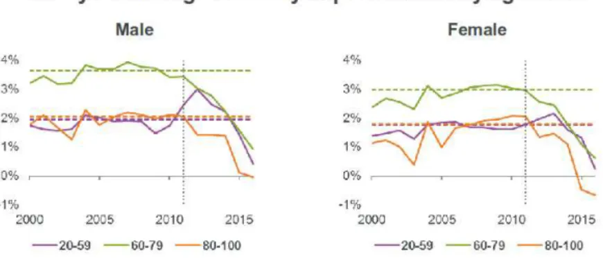
Although the emphasis is generally put on improvements in mortality, it is important to note that the data used for the CMI 2015 and CMI 2016 mortality projections show that the mortality improvements for the period between 2011 and 2015 are both lower for males and females, than for any five year period between 1976 and 2016 as shown in Figure 3.2.
Section 3.5. Future improvements in mortality Page 26
Figure 3.2: Average mortality improvement by age band. Source: CMI and SIAS(2017)
2015). Worst still at higher ages, the CMI’s analysis shows no improvement in the life expectancy at age 75between 2011 and 2015, as opposed to an “expected” seven months of increase.
Tim Gordon, Chairman of the CMI, said, ”Insurers and pension funds will need to consider whether this recent experience indicates a fundamental change in mortality improvement trends, or whether it is a short-term variation due to influences such as influenza and cold winters – the financial implications are material.” Source: https://www.actuaries.org.uk/news-and-insights/ media-centre/media-releases-and-statements/increases-life-expectancy-between-2011.
The question which arises is: is the recent fall in national mortality a blip or will it be persistent? Are pension schemes in a safe side updating their mortality assumptions with the new improvement rates? In a discussion hosted by the Staple Inn Actuarial Society and the CMI mortality projections committee on mortality improvements (CMI and SIAS(2017)), it was pointed out that the recent fall in mortality improvements can be partly explained by the reduced contribution to aggregate improvements from circulatory causes of death, e.g., heart diseases. Indeed in the period up to 2010, death rates from circulatory causes fell by up to 75%. Therefore, it is probable that the lower improvements are not likely to be temporary. Also it was suggested that socio-economic groups should be considered when setting assumptions, as the study shows that the slowdown in mortality improvements was not noticed amongst men with higher socio-economic class.
4. Analysis of Surplus
Another impact that a mortality experience has on a valuation is in the AoS. The AoS attempts to reconcile the last valuation’s technical provisions to the current valuation looking at the main factors that influenced changes in the scheme’s funding level. This is done by splitting the surplus (or deficit) into its components; which are differences between actual and expected experience for items related to assumptions made in the inter-valuation period.
A scheme with no surplus or deficit at the start of the valuation period will remain in balance if (cf. Chapter 21 of IFOA (2012)):
- all the assumptions, both financial and demographic hold as expected,
- the contributions paid over the period are those necessary to maintain the actuarial liability, - the assumptions used and the benefits valued in both valuations are the same.
In practice, however, it is improbable that everything goes as expected. Some sources of surplus (or deficit) are due to investment return experience, deficit contribution experience, normal contri-bution experience, withdrawal experience, salary increase experience, pension increase experience, commutation experience, post-retirement mortality experience. We can also analyse surplus re-sulting from benefit changes, ill-health/early retirement experience and change in contribution cost.
In this chapter, we shall focus on the post-retirement mortality experience, as an input to the AoS.
4.1
Reasons for an analysis of surplus and appropriate basis
to use
The AoS must be completed for every triennial valuation and is done for a number of reasons. First, it enables the actuary to make a semi-independent check on the current valuation relative to the results from the final basis in the last valuation. Also, this helps the actuary to recognise the potential significance of the assumptions chosen for the valuation. Moreover, the actuary can understand the reasons for any unexpected results and consider the likelihood of future repetition of such results, and advise the Trustees. The AoS is also a requirement by the pensions Technical Actuarial Standards for Reporting (TAS R), see Board for Actuarial Standards(2009).
In the case of a change in the assumptions adopted from those used in the last valuation, the analysis of surplus could be performed using either set of assumptions. However, there must be
Section 4.2. Analysis of surplus due to post retirement mortality Page 28
consistency in the assumptions and the values, used in the analysis of the current valuation and previous valuation. In most cases, and in our case study in Chapter 5, the approach is to calculate the current valuation’s result on the old basis. That is, we project the results of the previous valuation with the old basis to calculate the expected position on the old basis, then we explain the eventual existing difference between the actual position (current valuation on old basis) and the expected position.
The advantage of this approach is that it may help to set new assumptions since it reveals financially significant departures from the old assumptions. Also, it can help the Trustees to understand the significance of the change in assumptions.
4.2
Analysis of surplus due to post retirement mortality
This item on the AoS is entirely driven by the mortality experience analysis conducted for all the pensioners (retirees and dependants) in the inter-valuation period. The analysis can either be weighted by lives or by amount. Weighting by lives looks at the actual number of deaths experience against the number expected. However, the mortality analysis is usually weighted by amounts, i.e., it compares the actual amount of pension that has ceased to be paid, against the expected amount, considering the amounts that come into payment from spouse reversibility. In this way, the death of a member with a small pension will have little impact on the valuation as is expected.
An amount based experience analysis may also lead to the user setting different mortality tables for different groups of pensioners for the new valuation basis, where the groups are created considering the amount of pension in payment at the new valuation. For example, a different mortality table can apply to male members with a pension lower than £10,000 and another for
those above. The analysis also compares the spouse’s pension coming into payment with that which was assumed based on the proportion married, the spouse fraction and the mortality table. It is important to point out that more members dying than expected may not always result in a mortality gain, the spouse benefit which comes into payment on the death of the member must be taken into account, and the spouse can live for a more extended period than expected.
To formulate the gain (or loss) resulting from mortality more formally (as carried out in Willis Towers Watson, (WTW, 2015b), we let:
• x1 be the average age at death of actual experienced retirees deaths;
Section 4.2. Analysis of surplus due to post retirement mortality Page 29
• B1 and B2 be the total pensions in respect of the actual and expected deaths respectively;
• α%be the spouse percentage of member benefit; p%be the proportion married.
Then for an interest rate i, salary scale assumptionj, and considering the mortality tables in use, we have that
Gain/loss (G1) due to retirees post mortality experience is
G1 =B1
ax1i,j+α%p [ax1|y1 −ay1]
−B2
ax2i,j +α% p [ax2|y2 −ay2]
, (4.2.1)
where
y1 and y2 are the spouse ages, usually considered in standard practice, as the member’s age +3
for female members and member’s age −3 for male members; ax1|y1 is the contingent spouse annuity at average age of the actual deaths; ay1 is the surviving spouse annuity at average age of actual deaths. The same logic holds for the expected deaths.
For the members in the scheme which were already spouses (dependants), if we let
• x3 be the average age at death of the spouses actual deaths;
• x4 be the average age at death of the spouses expected deaths;
• B3 and B4 be the total pensions in respect of the actual and expected deaths, respectively.
Thus, the Gain/loss (G2) due to spouses post mortality experience is
G2 =B3 ax3 −B4 ax4. (4.2.2)
It is important to note that the dependants include both spouses and children. However, since very few children die during the inter-valuation period, a mortality experience study is not performed for them.
Therefore, the total surplus/deficit due to pensioners post-retirement mortality experience, G, is determined by summing the surplus(or deficit) resulting from both groups. That is