Near-rational expectations and the Phillips Curve : an empirical application

(1)

M

ESTRADO

ECONOMIA MONETÁRIA E FINANCEIRA

T

RABALHO

F

INAL DE

M

ESTRADO

DISSERTAÇÃO

N

EAR

-R

ATIONAL

E

XPECTATIONS AND THE

P

HILLIPS

C

URVE

:

AN

EMPIRICAL APPLICATION

J

OÃO MIGUEL CASANOVA NABAIS

(2)

M

ESTRADO EM

ECONOMIA MONETÁRIA E FINANCEIRA

T

RABALHO

F

INAL DE

M

ESTRADO

D

ISSERTAÇÃO

N

EAR

-R

ATIONAL

E

XPECTATIONS AND THE

P

HILLIPS

C

URVE

:

AN

EMPIRICAL APPLICATION

J

OÃO MIGUEL CASANOVA NABAIS

ORIENTAÇÃO:

MARGARIDA PAULA CALADO NECA VIEIRA DE ABREU

ISABEL MARIA DIAS PROENÇA

JÚRI:

Presidente: ANTÓNIO MANUEL PEDRO AFONSO

VOGAIS: EMANUEL GASTEIGER

ISABEL MARIA DIAS PROENÇA

MARGARIDA PAULA CALADO NECA VIEIRA DE ABREU

(3)

i

Abstract

The purpose of this work is to present and empirically test the Akerlof, Dickens and Perry (2000) model for two euro area countries, Portugal and Germany. The main purpose is to derive estimates for the Near Rational Phillips Curve and verify if the implications of ADP do apply to the current preference of the European Central Bank for an inflation target below the annual rate of 2%. Although no quantitative assessment is made over the adequacy of this target, we give some insight on whether this strategy is optimal for overall welfare.

Using annual data, we find evidence supporting the ADP conjecture that inflation is crucial for the degree of incorporation of price expectations in wage and price setting, although there is a weak link about its effect on unemployment, a finding which requires further study of the robustness of the Curve.

Keywords: Inflation, Unemployment, Phillips Curve, NAIRU, Natural Rate, Zero

Inflation, Monetary Policy.

(4)

ii

Resumo

O Objectivo deste trabalho consiste na na apresentação e avaliação empírica do modelo proposto por Akerlof, Dickens e Perry (2000) para dois países da Área do Euro, Portugal e Alemanha. Procurar-se-á deste modo obter estimativas para uma Curva de Phillips Quasi-racional e que verifiquem se os postulados ADP também são válidos em relação à preferência do Banco Central Europeu por um objectivo de inflação inferior a 2%. Conquanto não seja realizada uma análise quantitativa dos efeitos, procuram-se realizar breves reflexões sobre se a estratégia é óptima para o Bem Estar.

Recorrendo ao uso de uma base de dados anuais é possível encontrar evidência de que o nível da inflação é importante na determinação do grau de incorporação das expectativas na definição de salários e preços. No entanto, verifica-se uma fraca ligação entre esta e o desemprego, o que exige um estudo mais aprofundado sobre a sua robustez.

Palavras-Chave: Inflação, Desemprego,Curva de Phillips, NAIRU, Taxa Natural, Zero

Inflação Zero, Política Monetária.

(5)

iii

Acknowledgements

Completing this dissertation wouldn’t be possible without the support of various persons.

I would like to thank my supervisor Professor Margarida Paula Calado Neca Vieira De Abreu for her guidance, patience and motivation provided throughout the writing process, providing me with the faith to improve my skills, and to my co-supervisor, Professor Isabel Maria Dias Proença, for all the help provided with the use of the software package and the advice regarding the econometric implementation of the model.

I am also grateful to Thomas Dannequin, for his assistance in the reviewing and editing process.

I would also like to thank to all my Master’s Course colleagues Ariana, António Jossefa, Susana Matos, Sérgio Nunes, Teresa Margarida and Vasco Matias for sharing the good and, sometimes, challenging moments during the whole graduation process.

To all the members at Teatro da Universidade Técnica (TUT) for the exhilarating sessions and stage plays we have been to as an after-work cooler.

To Joana, my life force, for her caring patience, support, motivation and comprehension for moments postponed for carrying on with dissertation work.

Last, but not least, to my beloved Family – most closely, my Father, Mother and Sister - who put up with me during all these years of hard work and all the sacrifices they have made so that I could finish my academic studies. Especially I dedicate this work to the perseverance of my mother trough this most difficult year. May you find solace in this achievement.

(6)

iv

Recently, a new generation of Phillips Curve from Akerlof, Dickens and Perry (2000) (ADP) propose a return to its origins when a trade-off could be vastly explored from economic policy. Drawing their foundations from psychologists’ studies reporting the proneness of individual decision making to Money Illusion, they renewed the criticism over the issue of low-inflation targets as an unnecessarily constraint on Monetary Policy. Taking advantage of the positive effects of moderate inflation, they argue, would improve overall welfare.

In this work we proceed to empirically test the ADP model for two euro area countries, Portugal and Germany. The main purpose is to derive estimates and verify if the concerns of ADP do apply to the current preference of the European Central Bank for a low inflation target below the annual rate of 2%.

This study is divided as follows. In sections 2 and 3 we review the extensive literature on the Phillips Curve since its “humble” specifications, with an emphasis placed on the role of expectations.

In section 4, we present the theoretical underpinnings of the Akerlof - Dickens - Perry Model and its main innovations, while section 5 assesses its empirical performance.

Finally, section 6 concludes with the main findings, as well as future research paths.

(9)

2

2. The Phillips Curve Debate

2.1. The Phillips Curve is born

Although the study of the correlation between the movement of inflation and unemployment was pioneered by Fisher (1926), it was the seminal work of A. W. Phillips that brought the issue to discussion. Plotting the data of the United Kingdom for the 1862-1957 period, Phillips (1958) found that the rate of change of money wages was negatively influenced by the level and, to some extent, the rate of change of unemployment. This was possibly due to a “demand-pull effect” arising from the interactions between labour markets in an analogous way as demand and supply of goods and services: in times of fast business activity growth, firms sought to increase demand for labour, thus reducing unemployment and putting forward pressure for higher wage increases. Phillips also admitted the presence of non-linearities, as money wages displayed faster growth in booms, but fell slowly in recessions due to workers’ resistance “to offer their services at less than the prevailing rates” [Phillips (1958) , pg. 283]. These insights were further validated by Lipsey (1960), who developed a more robust theoretical model for a single labour market in which the length of the disequilibrium influences the speed of adjustment in wages. He also found evidence of a “cost-push effect” driven by the cost of living adjustments (COLAs).

Despite finding some shifts in the trade-off, Samuelson and Solow (1960) reached a similar conclusion for past historical data for the U.S. and suggested it should be used as a guideline for conducting fiscal and monetary policy, either by aiming for an unemployment rate target of 3% at the cost of price stability, or a price stability target of zero inflation and high unemployment around 5,5%. Other approaches to the Phillips

(10)

3 Curve can be traced to Perry’s (1964) inclusion of other variables such as the profit rate and the cost of living adjustments measures from previous periods, and Pierson’s (1968) analysis on the impact of the union’s bargaining power in the wage setting mechanism. Both infer in favour of the existence of a trade-off, although its size is reduced in the latter case.

2.2. The Natural Rate Revolution

A common disadvantage of early versions of the Phillips Curve was the instability of the size of the trade-off2, which exposed the fragility on theoretical

grounds and laid the ground for criticism. Most remarkable were the contributions of Phelps (1967, 1968) and Friedman (1968), which unified the diverse explanations with the introduction of two concepts: the natural rate of unemployment and the role of price expectations.

The first corresponds to the long-run equilibrium rate of unemployment, which happens when labour markets clear and of money wages grow at a steady rate.

Concerning Price Expectations, they work in the sense that, when negotiating wage changes, workers formulate their own expectations about the future path of prices to defend real purchasing power rather than its nominal value. Even if expectations are incorrect, they are gradually adjusted to offset the deviation error, ruling out money illusion.

Embedding these two features generated the Accelerationist Phillips Curve, whose equation is:

(1)

(11)

4 Where stands for inflation expected in the current period and for the natural rate of unemployment.

In the Short-Run, unemployment differs from its natural rate and the Phillips curve is negatively sloped. However, as soon as the economy approaches the natural rate, workers sense the pressure of labour demand and price increases and revise their expectations upwards, demanding higher wages. The result would be a higher wage increase and lower unemployment reduction, worsening the trade-off.

In the Long-Run, the Phillips Curve is vertical when unemployment equals the natural rate. Any attempts to further decrease unemployment have no other effect than to generate accelerating inflation, so the trade-off ceases to exist.

This approach stirred fierce opposition in the academic world , with Modigliani (1977) being a sound critic of the theoretical treatment of labour market dynamics3.

Empirically, since the natural rate hypothesis implied that the coefficient on inflation expectations equalled unity, it was common to proxy expectations with lagged values of inflation and testing whether the sum of its coefficients was significantly less than one, so that a permanent trade-off existed.

While these tests initially concluded favourably against the natural rate hypothesis, its credibility was challenged by Sargent’s (1971) critique, who claimed it was econometrically flawed because identification of its parameters could not be achieved due to the misspecification of the inflationary process as a unit root. Furthermore, evidence from Lucas & Raping (1969) and McCallum (1976) supported the validity of the Natural Rate Hypothesis, paving the way to a revolution that would irrevocably change the fate of the Phillips Curve Theory.

3

Modigliani voiced its concern mainly about the speed of adjustment, of which “(…) empirical evidence

suggests that the process of acceleration or deceleration of wages (…) will have more nearly the character of a crawl than of a gallop.” [Modigliani (1977), pg. 8]

(12)

5 2.3. Rational Expectations, Policy Ineffectiveness Proposition (PIP) and the demise of the Phillips Curve

The stability experienced throughout the 1950s and 60s ended abruptly with the dawn of the 70s. A surge in oil prices brought a combination of high, spiralling levels of inflation and rising unemployment hard to explain on the grounds of the Phillips Curve. In a series of influential articles, Lucas (1969, 1972) sought to explain this dilemma by complementing the Phelps-Friedman postulates with the concept of Rational Expectations4. Under this design, agents formulate their decisions based on

expectations drawn from all relevant information available. As a consequence, the effects of economic policy depend on whether they are anticipated or if they come as a surprise. While the first scenario doesn’t bring real effects on output and employment, the second generate short-lived fluctuations, which are quickly incorporated.

As regards the Phillips Curve, rational agents are completely free of Money Illusion – both in the short-run and long-run.

Within this framework, Lucas (1973) indirectly tested the Phillips Curve by using the Output- Inflation trade-off, showing a small, negligible effect on output with considerable increase in inflation. Thus, expansionary demand-driven policies were only met with negative effects of inflation, such as reduced real money balances and economic welfare.

What about the Phillips Curve relationship, as devised in the mainstream structural econometric models used for policy evaluation? In his groundbreaking critique, Lucas (1976) cast doubt over the validity of its parameters, since they didn’t

(13)

6 account for the role of the rational expectations in its formulation. As a result, the effects measured weren’t stable and were most likely subject to “parameter drift” over time, breaking down the predicted relationship. A formalization from Sargent and Wallace (1976) confirmed many of Lucas’ conclusions and presented the Policy Ineffectiveness Proposition (PIP):

“In this system, there is no sense in which the authority has the option to conduct

countercyclical policy. To exploit the Phillips Curve, it must somehow trick the public. But by virtue of the assumption that expectations are rational, there is no feedback rule that the authority can employ and expect to be able systematically to fool the public. This means that the authority cannot expect to exploit the Phillips Curve even for one period.”

[Sargent and Wallace (1976), pps.176-177]

Barro (1976) also noted that, even when monetary authorities have superior information on the economy but agents do not, movements produce real effects unless information is provided.

The rational expectations revolution marked a shift in the Macroeconomics discipline. The Phillips Curve, described as an “econometric failure on a grand scale5”, was reduced to the “wreckage” of the bulk of the obsolete Keynesian models. Demand policy management was cast aside in favour of Supply-Side models of Real Business Cycles (RBC). Built in the spirit of the “Lucas Research Programme”, their foundations rested in the rational, optimizing behavioural nature of agents in order to study the causes of the fluctuations in business cycles.

(14)

7 2.4.The New Keynesian School and the resurgence of the Phillips Curve

No sooner had Rational Expectations taken over the macroeconomics disciplinethat some authors started casting doubt about the PIP.

The main argument came first from Fischer (1977), Phelps and Taylor (1977), and Chadha (1989) who pointed out that agents usually resort to multi-period contracts for setting the nominal value of wages and prices. This fact induces “stickiness” in these variables that leads to a sluggish adjustment in response to frictions from demand and supply, producing real effects in output and employment and allowing for a role of stabilizing monetary policy, as Ball, Romer & Mankiw (1988) and Mishkin (1982) testify. This marked a renewed interest in the resurgence of a Keynesian counter-revolution known as New Keynesian Economics, divided in two schools of research.

One version of the New Keynesian Economics rests on RBC Theory in the Lucas-Sargent-Prescott tradition. This line of research merged the rational expectations of the New Classical School with Keynesian micro foundations of imperfect competition and nominal rigidities in price and wage setting responsible for incomplete nominal adjustment.

The main contributions came from staggered contract models from Taylor (1980), Calvo’s (1983) random price adjustment, and the quadratic price adjustment cost from Rotemberg (1982)6. For the purpose of modeling inflation dynamics, Roberts

(1995) shows that these models share a common concept of price stickiness that allowed to derive what we call the New Keynesian Phillips Curve (NKCP), whose baseline equation is:

(2)

6_{A third family of price stickiness models, known as “Menu Cost”, is drawn from Akerlof and Yelen (1985),} Mankiw (1985) and Blanchard and Kiyotaki (1987).

(15)

8 Where π stands for inflation, Et is the current period’s expected value operator for the formation on inflation expectations and the deviation for marginal cost.

This formulation resembles the Phelps-Friedman Accelerationist approach, allowing for a short-run trade-off expressed in terms of output-inflation. Despite its appealing formulation, there has been an ongoing debate concerning the adequacy of its forward looking formulation and how to measure deviations in marginal cost, since it isn’t directly observable.

For instance, Fuhrer (1995) argued that forward-looking behavior not only is irrelevant, but also gives a poor empirical performance of the model. In addition, Roberts (2005) also show that backward-looking expectations are relevant. In order to shed light over this issue, a new structural formulation of the NKPC split the formation of expectations’ process between forward and backward looking components. This formulation, known as the Hybrid New Keynesian Phillips Curve (HNKPC), was followed by Fuhrer and Moore (1997) by setting equal weights. Galí and Gertler (1999) and Galí, Gertler and López Salido (2001) allowed the weights to be determined within the model, and found evidence that Europe and US were predominantly forward looking.

But the main disagreement is about the real marginal cost term. One natural candidate is the output-gap, detrended to exclude cyclical fluctuations, a procedure followed by Roberts (1995).

However, Galí and Gertler (op.cit) and Galí, Gertler and López-Salido (op.cit) claim it to be an unsuitable choice, due to the fact that natural output is a latent variable, resulting in considerable measurement errors. Instead, they propose the use of real unit labor costs as a proxy to define the Labor income Share impact to the inflation process,

(16)

9 an approach also followed by Sbordone (2002). Nonetheless, Neiss and Nelson (2005) and Roberts (2005) show that some output-gap based measures yield plausible estimates for the NKPC.

In some empirical works the rational expectation hypothesis has been relaxed and direct survey data on inflation have been used, with the intention of allowing a degree of non-rationalities. Following this approach, Roberts (1995) and Adam and Padulla (2003) obtained better results for the U.S. NKPC with output gap, while Paloviita (2006) shows that Euro Area inflation dynamics perform better with an HNKPC, displaying a predominant backward looking behavior that has been giving way to forward looking behaviour in recent years of low inflation. Also the choice between output gap and labor income share seems to be irrelevant, with both displaying a good empirical fit.

A remark from Romer (1993) brought the possibility that the degree of openness of an economy, measured by the average GDP import shares, might influence the slope of the Phillips Curve in a negative fashion. Although Temple (2002) argues the connection isn’t clear cut, some extensions have been made to the NKPC to reflect the impact of external trade. Examples of these can be found in Galí and Monancelli (2005) and Mihailov et al. (2011) by adding a term reflecting the terms of trade improvement, which play an important role in determining inflation dynamics.

In a different approach, Leith and Malley (2007) and Rumler (2007) propose a different model where the open economy is present in the form of a consumption choice between domestic and foreign goods, and imported intermediate goods and labor are substitute factors of production. However, while the model fit turns out better than in the closed economy case, the slope doesn’t seem to be affected.

(17)

10 Whereas criticism aimed at the fragilities of the Phillips Curve was openly acknowledged, some economists called for a re-specification of the mainstream equation, rather than casting it aside. This group of New-Keynesian Economists, whose main contributions have been drawn from the works of Modigliani and Papademos (1976) and Gordon (1977, 1982), present an Accelerationist Phillips Curve in the following form:

(3)

Where , and are polynomial operators for lags and is a serially- uncorrelated error term.

This equation constitutes the “Triangle Model of Inflation”, due to the three determinants that influence inflation dynamics: inflation Inertia, represented by the inclusion of lagged values of inflation, starting at (which come also as a substitute

of expectations); Excess Demand , usually measured by the unemployment gap, 7_{; finally,} _{represents a vector of supply-shocks variables such as import}

prices and the price of food and energy, whose occurrence is transitory by nature and normalized to zero ( ).

While the two first components are meant to capture the rate of change and slow adjustment effects, the last term is the key innovation of the Triangle Model, for it explicitly recognizes a “cost-push” effect which had been previously omitted in Phillips Curve specifications.

With the separation from the main driving force of inflation in the 70s and 80s decades, the core Phillips inflation-unemployment relationship was restored under the stability of its parameters and provided a short-run trade-off in the tradition of

7

(18)

11 Friedman-Phelps natural rate hypothesis. And the development of new econometric methods and statistical software packages perfectly suited the focus placed on obtaining estimates for a Non-Accelerating Inflation Rate of Unemployment (NAIRU)8 consistent

both with steady inflation and the absence of supply shocks - the “no-supply shock

NAIRU”.

2.5. Strengths and Weaknesses: which model suits best?

Instead of an epitaph, the Lucas-Sargent post-mortem statement backfired into a New Keynesian Economics framework, with a two-way bifurcation in Phillips Curve conceptions.

Being different in theoretical foundations, each gave their contribution in an intellectual environment characterized by growing interest in the use of monetary policy as an effective stabilizing tool and the advent of inflation targeting strategies around low levels of inflation.

The NKPC approach placed the focus upon the formation of expectations, how they react to changes in policy and their effects in the inflationary process. Their findings gave support to the importance of the Governance Structure of Central Banks for sound credibility and independence in the conduct of monetary policy, a feature which proved empirically relevant in explaining the end of hyperinflation episodes and providing low volatility in fluctuations. For this reason they have been labbeled as the “workhorse in discussions of fluctuations, policy, and welfare9_{”. Nonetheless, there’s}

still a great degree of skepticism regarding the limitations for the use of these models. A wide range of tests conducted by Rudd and Whelan (2007) provide a strong criticism

8

While it is usual to assume that NAIRU and natural rate are equivalent concepts, it has not always been the rule. For instance, Tobin (1997) separates the two concepts by defining the former as a market-clearing equilibrium and the latter achieved in a disequilibrium framework. Here I decide to interpret the Natural rate purely as a central theoretical concept, while the NAIRU and its counterparts as derived within a model.

9

(19)

12 against the robustness of the results of the NKPC and HNKPC. The main problem arises from the choice of proxies for marginal cost, where labor share measures display countercyclical behavior with inflation, rendering it an inadequate alternative choice.

When compared to the Triangle version of the Phillips Curve, the NKPC has two important drawbacks: First, the model doesn’t recognize an explicit role for supply shocks, which are simply relegated to the error term10. Moreover, the trade-off is

expressed in output-inflation terms, which doesn’t allow obtaining NAIRU estimates11,

thus limiting its scope as a policy guidance tool.

The approach delivered a stable, well defined Phillips Curve which fitted well in postwar inflation dynamics. These properties guaranteed the Triangle Model a place in the mainstream approach in assessing the conduct of monetary policy through its goals for price stability, as can be seen by the vast literature reporting point estimates of the NAIRU12 .

Nonetheless, this approach had an important drawback: since the natural rate is a theoretical construct, it has an unobservable nature of a latent variable where the NAIRU plays the role of a mere numerical estimate. But, as Staiger, Stock and Watson (1997a, 1997b) show, assuming a constant NAIRU value of 6,0% in the computation of these estimates revealed a high degree of imprecision in its measurement, due to the presence of high standard errors and wide confidence intervals. This result suggested that the NAIRU could be moving over time, due to changes in the behavior of labor markets. This observation dates back to Perry’s (1970) interpretation that modifications in the demographic structure of the labor force could influence the

10

Hooker (1996) and Blanchard and Galí (2007) counter this argument by arguing that the input share of oil and other energy prices has decreased since the first shocks in the 1970s, due to a myriad of factors.

11

Galí (2009) provides a new specification for a New Keynesian Wage Phillips Curve, where wage inflation is expressed in terms of unemployment, just like the original Phillips equation. Unfortunately the author does not report NAIRU estimates.

12

For instance, see Gordon (1988), Wiener (1993), Fuhrer (1995) and Tootell (1994) for the US and Marques (1990), Luz e Pinheiro (1993) Gaspar e Luz (1997) e Marques e Botas (1997) for Portugal.

(20)

13 NAIRU, a conclusion also corroborated by Shimer (1999) and Katz and Krueger (1999).

Other explanations have been put forward, such as beneficial supply shocks originating from technological progress - Gordon (1998) - and increased labor productivity growth - Ball and Moffitt (2001), Ball and Mankiw (2002). Cohen, Dickens and Posen (2001) also emphasize the role of new methods in human resources management and the surge of job-matching services over the Internet in increasing matching efficiency in labor markets, while Blanchard and Summers (1986), Blanchard and Wolfers (2000) explore the impact of unemployment hysteresis (i.e. the persistence of a? high unemployment rate(s?) through long periods of history) on the evolution of the NAIRU.

While the debate is still ongoing13, the time-varying NAIRU issue has been

acknowledged by apologists of the left-fork approach, who allowed parameter variation and structural breaks in order to identify its trends. Examples of these treat movements in the NAIRU as deterministic throughout time [Staiger, Stock and Watson (op.cit.) and Cross, Darby and Ireland (1997)], or displaying stochastic uncertainty [Gordon (1997, 1998), King, Stock & Watson (1995) and Laubach (2001)], along with the decomposition of unemployment in short and long-term [Llaudes (2005)].

Another common approach combines this latter specification with other equations in order to achieve better identification of NAIRU estimates. Such examples can be found either by joint estimation with an Okun Law’s equation, as followed in Apel & Janson (1999), Fabiani & Mestre (2001) and Basistha & Startz (2004), or matching a Triangle Phillips Curve with the jobs vacation-unemployment stated by the

13

Blanchard and Katz (1997) and Katz (1998) sought to unify these different approaches under an approach known as Supply, Demand and Institutions (SDI) model. See Banco de Portugal (2009) for an empirical example for Portugal.

(21)

14 Beveridge Curve, as presented in Dickens (2008). This system-based approach resulted in better precision in its estimates.

Overall, these studies confirmed the changing nature of the NAIRU and were able to track its evolution in the post-war period: in the United States it was low in the 60s, rose in the 70s and 80s and declined in the 90s14. Low values also characterized the

NAIRU in Europe during the 60s, but rising unemployment during the 80s and 90s resulted in higher values since then15. Still, the uncertainty of these estimates remains an

issue to be tackled with and gives reasoning for reducing its weight in the formulation of optimal monetary policy rules16 or dismissing the utility of NAIRU based models17.

3. Departure from the Natural Rate Hypothesis

As we’ve seen, three important concepts have been firmly “grounded” in the Phillips Curve literature: the role of expectations formation – rational and adaptive –, the existence of a natural rate of unemployment and the absence of money illusion. These features allowed a linear trade-off between inflation and unemployment that would endure in the short-run, dissipating as unemployment approached the NAIRU. And they eventually made their way in the design of Monetary Policy Rules by the majority of Central Banks around the globe, who recently shifted to an Inflation Targeting Strategy, whose formal commitment to pursuit a publicly announced target of inflation at low levels was a fundamental condition for a stable macroeconomic environment. While the experience is often lauded as successful, some concerns have been raised over this approach to monetary policy.

14

This decade was also characterized by a strange phenomenon of low inflation and low unemployment in the U.S. the United Kingdom. An explanation is advanced in Gordon (1998).

15

Ireland and Portugal are detached examples of this group, showing declining and stable values of the NAIRU, respectively. See Browne & McGettigan (1993) and Dias, Esteves & Félix (2004) for possible explanations of this fact.

16

Meyer, Swanson & Wieland (2001). In a different perspective, Stiglitz (1997) and Estrella & Mishkin (1999) argue that one should look at the NAIRU not as an achievable target, but as a short-run construct of the natural rate that uses current and past economic indicators for forecasting the future path of inflation.

17

(22)

15 One is labelled the lower zero bound of nominal interest rates. Because inflation has decreased, there was enough margin left for a nominal interest rate reduction in order to achieve a lower real interest rate. In low inflation environments, though, there is a greater risk that an adverse shock might cause deflation, which is a highly undesirable outcome18. Also, despite much research pointing towards a negative

relationship between inflation and economic growth19, Bruno and Easterly (1996) and

Bullard & Keating (1995) claim this linkage is weak in low inflation environments. The other concern focuses on the welfare implications of higher unemployment arising from pursuing a low inflation objective. Comparative studies by Feldstein (1997), Dolado et al. (1997) and Tödter & Ziebarth (1997) argue that the long-term gains in output and reduction of distortionary effects arising from taxation are well worth the short-term costs of a disinflationary process.

Yet, as Ditella et al (2001), Wolfers (2003) and Blanchflower (2007) report, unemployment causes more unhappiness than inflation, showing that public opinion emphasizes the hidden costs of unemployment (psychological, loss of personal revenue, etc.) which are eager to create strains in social cohesion.

Matching these statements with the findings of King & Watson (1994), Fair (2000) and Karanassou et al (2003), all reporting the existence of a long-run relationship between inflation and unemployment in the United States and Europe, one has to wonder whether Tobin’s (1972) observation of some features in wage behaviour which allow for a reduction of unemployment beyond the (un)natural rate, without incurring the “inflationary bias”.

18_{Detailed studies about the effectiveness of monetary policy in low inflation can be found in Fuhrer &}

Madigan (1997), Cohenen et al. (2003) andReifschneider & Williams (2003);

(23)

16 3.1. The Akerlof, Dickens & Perry Model I - Fairness and Downward nominal wage rigidity

Tobin’s challenge was promptly answered by Akerlof, Dickens & Perry (1996). Analysing the distribution of wage changes, they observed that nominal wage cuts are rare and mostly remain unchanged. This pattern reveals the concept of Fairness in wage setting: workers are resistant to nominal wage cuts and firms, afraid of the consequences of losing the best employees and reduced work effort, avoid resorting to this option unless their survival is at stake. This induced downward nominal wage rigidity – i.e. wages are flexible upward but downwardly rigid - constrains firm’s reaction to adverse shocks and results in higher unemployment, an effect magnified when inflation is lower than 3%. The underlying Phillips Curve displays a non-linear shape, allowing a long run trade-off and an equilibrium rate of unemployment consistent with steady inflation – the Lowest Sustainable Rate of Unemployment (LSUR) – lower than the NAIRU.

This work revived the discussion over the upward revision of inflation targets from a low, near-zero inflation, to a price stability target consistent with the LSUR, in order to take advantage of “grease” effects of inflation on the labour market.

For the United States, Card & Hyslop (1997), Groshen & Schweitzer (1999), McLaughlin (1994), Kahn (1995), agree on the existence of some downward stickiness in nominal wages but the positive “grease” effect of higher inflation is reduced to modest gains20 due to the negative “sand” effects. On the other hand, Sargent & Stark

(2003) and Knoppik & Beissinger (2003) find it to be strong in Canada and Germany, respectively.

20_{Akerlof, Dickens and Perry are well aware of these results, but they warn the presence of measurement}

errors that correction procedures are unable to eliminate. Card and Hyslop do not even attempt to correct it, thus retiring power as persuasive evidence. Using another data source, Lebow et al (1999) find strong evidence of downward wage rigidity, though it doesn’t bear significant changes on the Phillips Curve.

(24)

17 Overall, the reliability of data sets used in these studies seems to influence results. However, according to Holden (2002), a central aspect explaining country differences in the relevance of this phenomenon rests upon the institutional framework of wage bargaining.

3.2. Formation of Expectations Vs Incorporation of Expectations – Money Illusion and Heuristic Bias

Since the groundbreaking Friedman-Phelps-Lucas contributions, formation of inflation expectations has played a central role in Phillips Curve Theory. Either through adaptive or rational expectations, agents made the best use of available information so it was assumed that agents fully understood the implications of inflation. In doing this, they neglected a fundamental issue: how do agents incorporate their knowledge into decision making? Does human decision-making mirror the wisdom of the Economics Profession?

On this issue, evidence drawn from psychological studies shows a blurry picture. A survey conducted by Shiller (1996) on the perceptions of the inflation process shows that inflation is acknowledged by the mainstream public as harmful increase of prices that lowers real income, an attitude that is especially salient in generations who experienced episodes of high inflation. Apart from this aspect, confusion and misconceptions about its causes and impact on the overall performance of an economy seems to be the norm: few people associate it as a central feature of interactions between wages and prices or between demand and supply, as well as other issues such as macroeconomic volatility, redistribution of income, etc.. A concept of Fairness is also present both in a negative fashion - associated when inflation is regarded as a result of “corporate greed” in the pursuit of easy profits - and, ot some extent, in a positive perspective – higher prices are tolerable as long as income keeps up with the pace.

(25)

18 The last statement exhibits the frame-dependence of opinions upon the context in which the inflation problem is formulated. But it also highlights the presence of another cognitive bias: Money Illusion, i.e. a tendency to put more weight in the nominal value of contracts rather than its real term, when evaluating economic decisions. An extensive survey conducted in Shafir, Diamond and Tversky (1997) show how agents are often misled by nominal anchoring when formulating decisions covering simple transactions or even more complex ones, such as Wage Indexation, Portfolio Investment and Accounting standards. Again, the ambivalence of decisions which characterizes frame dependence has an influence in amplifying Money Illusion, whose main outcome reveals underestimation of inflation.

These phenomena described above strongly suggest that non-economist agents adopt a mental accounting that closely follows simple “rule of thumb” models, which are more likely to be subject to cognitive errors. Consequently, incomplete incorporation of inflation expectations and inconsistency of preferences and non-maximizing behavior arise, violating the basic tenet of Rational Expectations theory.

In fact, learning processes fit more closely the conclusions reported by cognitive psychologists on heuristic errors and configure another concept suggested by Akerlof & Yellen (1985): Near Rational Expectations. This postulates that deviations from rationality entail only small costs for agents so they do not have an incentive to adjust at the microeconomic level; at the macroeconomic level, however, this suboptimal behavior is a cause for fluctuations.

3.3. The Akerlof, Dickens & Perry model II – Near Rationality and the (Behavioural) Phillips Curve

Under this setting, Akerlof, Dickens & Perry (2000) draw a multi-agent approach in which a proportion of near rational agents disregard inflation from wage

(26)

19 and price setting in low inflation environments. This “information edit” allows for less than complete incorporation of inflation in expectations and keeps up with the fact that its coefficient is prone to change through time and is positively correlated with inflation21. They derive a nonlinear Phillips with an unusual shape: it is vertical at the

NAIRU at very high levels of inflation, but backward bending at low and moderate rates of inflation. This allows a Long Run trade-off between inflation and unemployment within the 1,6%-3,4% inflation range. Once more, estimates of the LSUR are lower than predicted by NAIRU models by a difference of 1,5% to 3,1%, implying that there is more room for obtaining gains in employment without pushing inflation to harmful levels. Similar results are obtained for Canada in Fortin (2001), for Sweden in Lundborg & Sacklén (2006) and Maugeri (2010) for Italy. Given the current inflation targets set by the respective Central Banks, these results point out that currently monetary policy is undesirably contractive.

In short, research in Phillips Curve theory has taken a long path. Five decades have passed since the original Phillips Curve turned into a cornerstone of macroeconomic theory and, given the fact that its two main contributions – the role of expectations in price and the natural rate of unemployment – decisively marked most of its path as a linear short-run relationship, new directions return it to the nonlinear relationship and Long Run Trade off presented in Phillips original work. One can resort to the 15th century navigator’s goal of reaching India either by navigating West or East

as an allegory to explain the lack of consensus in the foundations of Phillips Curve Theory. By choosing an intermediate path between the two, but with a different perspective, this generation of ADP Phillips Curve proposes to “circumnavigate” the World of the Phillips Curve with a groundbreaking contribution – one where the limits

(27)

20 of cognitive ability in human behavior affect the incorporation of the economics and model imperfect information gathering in order to provide better foundations for economic theory22.

4. The Akerlof-Dickens-Perry Model

4.1. Theoretical Foundations

We now present the model Akerlof, Dickens & Perry (2000) used to derive the Near - Rational Phillips Curve. Starting with the macroeconomic behavior, income follows the quantity theory equation:

(4)

In which represents average price level in the economy, is nominal income and stands for Money Supply. Aggregate Demand in the economy is then determined by the real money stock in the economy and it can be extrapolated into a microeconomic setting in which firms operate in a Monopolistic Competition Framework. In this context, demand for a single firm’s output depends on the price they charge relative to the average price level:

(5)

Monopolistic competition endows a firm with some power market power in price setting, which materializes in a mark-up charge over their production costs23. But in the

pursuit of profit maximization, they will bear in mind the impact of wages on workers’ productivity - which calls the theory of efficient wages into our model. According to it,

22_{The notion that information costs can have important effects in the macroeconomics of inflation and}

unemployment is motivating further developments see for instance, the example of Sticky Information provided in Mankiw-Reis (2002).

23

Besides Labor, ADP doesn’t mention other costs involving other factors of production. For the purpose of simplicity, we will only consider wages as relevant to our model;

(28)

21 a firm must pay an efficient wage that takes into consideration the workers’ perception of “Fairness”, that is, a reference wage he or she expects to receive as acknowledgement of his efforts and outside job opportunities. The productivity expression will then be defined as:

(6)

Where and are the wage paid and the reservation wage, is aggregate unemployment and , , and 1. The ratio is the crucial component for unit labor cost minimization. Firms cannot directly observe , but will try do so by adjusting wages at the rate of the inflation expected for the next period, given the nominal wage currently paid, leading to the following wage setting rule:

(7)

Where is the average nominal wage, the inflation expected for the next period and assumes a value between 0 and 1. In this process, however, some firms and workers may be induced by “money illusion” and do not fully incorporate expectations in the wage setting process. In this case, and we say these agents have “near-rational” expectations, in contrast to rational agents that fully incorporate expectations ( ).

The problem the firm faces will be:

According to the efficient wage theory, the first order condition is achieved when marginal productivity relative to wage equals unity. That is, it must satisfy:

(29)

22

Solving the problem in order to the nominal wage , we obtain the following expression:

(8)

Where j identifies the agent as near rational or fully rational .

The profit-maximizing choice for the firm will be a constant mark-up ( )over unit labor costs:

(9)

Through expressions (6) and (7), we are able to discern the main innovation of the model: near rational workers end up earning a lower wage which in turn will be reflected in lower prices charged by firms. Once true inflation kicks in, both will suffer losses in real income from wages and profits. Focusing the consequences on the latter, the loss function of relative loss profit faced by a near-rational firm could be written as:

(10)

With and representing the profits earned by the rational and near-rational firm and the ratio of “cost push” differential. When inflation is zero, 1 and no losses are incurred; for low values the losses are so small that there is no incentive for a near rational firm to change its behavior towards full rationality. However, as inflation rises, losses will also increase and this incentive will eventually fade, up to a threshold of magnitude . Assuming they are normally distributed, i.e. a , the proportion of near-rational price setters will be given by:

(30)

23

(11)

This encloses the theoretical model. We will now show how ADP proceeded to derive the Near Rational Phillips Curve.

4.2. The Near Rational Phillips Curve

How does Near Rational behavior impact upon the Phillips Curve? At the macroeconomic level, the aggregate wage level will then be determined as a weighted average of prevailing wage levels:

(12) Substituting (7) and (8) in (12), we get:

(13)

To express this equation term in differences, we divide both sides by and

rearrange in order to obtain (14):

(14)

Where stands for wage inflation. Finally, taking logs on both sides and following the approximations made by ADP generates the short - run wage Phillips Curve,

(15)

Where is a constant and .

The implications of near rational behavior on equation (15) are straightforward: will be less than one and incomplete incorporation of inflation expectations occurs as

(31)

24 long as inflation is low, enabling a long-run trade-off between inflation and unemployment. However, as inflation rises, more agents will perceive the effects of higher inflation and switch their behavior towards full rationality, increasing and progressively reducing the trade-off. At a sufficiently high inflation rate, and the coefficient on expectations equals unity. Since inflation is now fully incorporated,, we may set and the Phillips Curve becomes vertical again at the natural unemployment rate . This would rewriting equation (15) as:

(16)

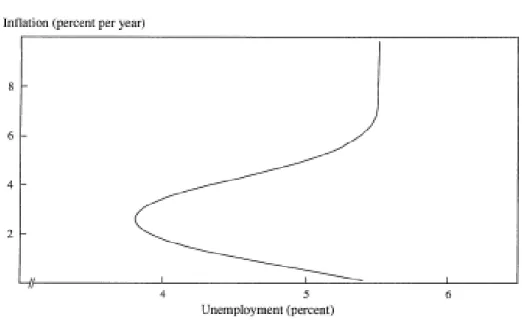
The underlying Phillips Curve takes the backward-bending form as reproduced in Figure 1. It is vertical when unemployment is at the natural rate , which happens when inflation is zero or above six percent. Between this range, though, it is possible to bring unemployment below the natural rate with only modest increases in inflation, eventually achieving the optimal rate – the Lowest Sustainable Unemployment Rate (LSRU) – between 2%-4%.

Figure 1: An hypothetical Phillips Curve 1

(32)

25 This argument has important implications for today’s policymaking debate, especially in Europe. With the European Monetary Union in place, along with a Monetary Policy whose aim is to stabilize inflation around the 2 percent target, a Phillips Curve with the shape of figure 1 would generate unnecessary higher unemployment when price stability could still be satisfied at moderate rates of inflation. To this end, we chose to individually pick Germany and Portugal to empirically assess the existence of such Phillips Curve. The main rationale behind our choice is that, in the presence of a trade off in Germany - whose outcomes weight heavily upon the course of the European Central Bank (ECB) - then a small open economy such as Portugal can also benefit from it. Below we present some descriptive statistics on key variables averages over time:

Table 1: Summary Statistics - Germany

Period Inflation CPI Inflation GDP Deflator Unemployment (age) Unemployment (CL) 1964-1974 3,77 n.a. 1,08† 0,99 1975-1986 5,90 6,73 5,16 5,20 1987-1995 3,59 4,19 6,65 6,67 1996-2000 1,25 -0,66 8,88 8,88 2001-2011 1,61 0,99 8,46 8,62

Source: OECD †Data availableonly for 1970-1974. n.a. non-available

Table 2: Summary Statistics - Portugal

Period Inflation CPI

Inflation

GDP Deflator Unemployment (age) Unemployment(CL)

1964-1974 8,50 6,29 n.a. 2,56

1975-1986 19,54 5,29 7,18 7,62

1987-1995 8,61 5,56 5,70 5,60

1996-2000 2,64 2,83 5,72 5,46

2001-2011 2,52 2,20 8,44 7,84

(33)

26 At first glance, the differences in inflation between the two countries are obvious. Here, Germany’s renowned commitment to low inflation has resulted in maintaining a stable historical rate of inflation, despite events such as the oil prices shocks in the mid-1970s and 1980s and the German reunification in 1990.

In contrast, Portugal’s macroeconomic instability during the 1970s and 1980s forced the country to apply for two IMF-relief assistance (one in 1977 and another in 1984) programs and to undergo exchange-rate devaluations that caused spiraling inflation. Eventually, despite the strain created by the 1992-1993 European Monetary System crisis, the efforts to tame inflation had finally succeeded and the country applied for euro membership, enjoying since then a relative stability in price dynamics.

Regarding the developments in the labor market, Portugal displayed lower unemployment rates than Germany throughout the second andhalf third tier of the twentieth century and evaded the hysteresis unemployment occurring in Europe, although the first ten years of the 21th century signaled a reversal of this trend.

Intertwined, we cannot detach the existence of a sound trade-off for Portugal until the first decade of the 21th century, but for Germany it is more apparent throughout

the periods analyzed.

4.3. Empirical Specifications

In order to derive de Price Phillips Curve, Akerlof, Dickens and Perry (2000) allow for the introduction of unemployment lags in equation (15) to reflect the impact of changes in unemployment term, since it will also affect wages and labor productivity in the model. They also use the approximation for the profit loss function to circumvent the need to estimate parameters , , and . Following these procedures, the empirical version of the Short Run Phillips Curve will be given by:

(34)

27 (17)

Where is the price level inflation, stands for the intercept term, the cumulative standard normal density function representing the fraction of rational agents in the economy, represents the effects of past inflation on agents rationality, stands for inflation expectations, and represent lagged terms of

unemployment, is a vector of time dummies accounting for supply shocks events and the error term. Accordingly, , , , , and are the parameters we wish to estimate.

At first glance, equation (17) closely resembles the standard Accelerationist version of the Phillips Curve. The main difference, however, nests within the coefficient on inflation expectations, which is now a non-linear function between a constant and past inflation.Were the expectations to follow the pattern described by the Natural Rate model, then only would matter for expectations and also assume a high value; In the ADP framework, though,the coefficient embodies a central feature of this process. If it is positive, then is increasing in inflation, as a larger share of past inflation will be incorporated in the expectations process.

In the long run, expected inflation equals actual inflation ( ), unemployment is constant ( ) and shocks are absent ( and

). Expression (17) then becomes the Long Run Phillips Curve: (18)

Which we can solve in order to : (19)

(35)

28 The common procedure adopted in ADP (2000) and followed in similar studies consists firstly in estimating equation (17) and then using the estimated parameters to numerically compute the Natural Unemployment Rate24, the LSUR and the LSURI

through expression (19). Albeit intuitive, Maugeri (2010) notes that this exercise bears the objection that the coefficients estimates might not be invariant in the Short Run and Long Run, suggesting a cointegration approach to circumvent it.

4.4. Data Set and Variable Construction

Currently, existing ADP Phillips Curves have only been estimated using quarterly data to increase the range of available observations; since we are more interested in analyzing the existence of a Long-Run Relationship over a time span, short-run fluctuations might introduce some disturbance that might be unnecessary for the purpose25. For this reason, and to experiment with a different range of data, we have

decided to set the frequency of data to annual, and all the quarterly-period specifications in ADP have been equivalently converted to this context. The sample data traces back to the mid 1960s until 2011, but since the starting data length is shorter for some variables, we are only able to gather between 28 and 44 observations.

When regarding Inflation as a concept, one must be careful of the limitations arising from the use of a single indicator. It is hard to accurately measure inflation, and it is common practice in the economic literature to employ several indicators when estimating a Phillips Curve. Amidst all the measures used in ADP, a natural candidate is inflation measured by changes in the CPI26. Lundborg & Sácklen (2006) note, however,

that core CPI may be misleading for small economies, because they are extremely

24_{From expression (19) this value is reached either when and inflation is zero (} _{) or when it}

is high enough so that the cumulative standard normal distribution is equal to unity.

25

Here we decide to follow the point made in Wyplosz (2001);

26

We also bear in mind that CPI is not comparable between countries, due to differences in the calculation - most namely, the composition of the goods basket.

(36)

29 vulnerable to fluctuations in the terms of trade. Because we lack an Import Price Index to isolate these effects from CPI like they do, we also use changes in the GDP deflator to fulfill the same purpose as measure of domestic inflation.

To proxy , several specifications are advanced by ADP. We decided to restrict to the following weighted rule:

(20)

Where is estimated either unconstrained or in restricted form ( ) with I set to 4 periods. For , we also follow the adaptive expectations’ tradition of using lagged values of inflation, either by following (18) with set to 3 periods or defining an arithmetic average27 of the lagged past 3 observations. However, as we have

referred, this approach might not be representative of the process in which expectations are formed and direct measures of inflation expectations are required as a better account. In this approach, we followed the suggestion of Wyplosz (2001) and assembled a “Consensus Forecast”, consisting in the average of one-year ahead Inflation forecasts from the OECD’ December issue of the Economic Outlook and the Autumn Forecasts from the European Commission.

While more straightforward, the concept of unemployment has evolved over time and its series have also been subject to frequent methodological changes. We have therefore decided to follow the same approach of multiple measurements for unemployment. For this, we first picked two measures of Total Unemployment - aged 15-61 and as a percentage of the Civilian Labor Force – and, at a later stage, Unemployment of Male Workers aged 25-64.

(37)

30 When it comes to estimating equation (17), we sought to exploit a? different combinations? of the indicators mentioned above with one of the two methods which have been employed so far. ADP, Dickens (2001) and Maugeri (2010) used Non-Linear Least Squares, while Lundborg & Sacklén (2006) opted for Maximum Likelihood methods. The latter method tends to produce more efficient estimates than the former but, due to convergence problems of the Likelihood function, I was unable to derive estimates for the equation. Fortunately, Non-Linear Least Squares performed pretty well with the majority of our specifications, which we reproduce in the next section.

5. Results

Table 3 and Table 4 in the annex present the results for four estimations of ADP Near-Rational Phillips Curves. For each country we have plotted the three best regression results, along with a “least successful” case28. The main conclusions for each

regression are summed up below.

5.1. Germany

Overall, the German Phillips Curve performs better when inflation is measured by changes in CPI and the estimates follow closely those reported in ADP (2000) and Lundborg &Sackén (2006). However, when compared with Dickens (2001) results for Germany, the picture changes considerably. For instance, the intercept term in our regressions is always positive, while Dickens (2001) reports the opposite. In the light of the Phillips Curve, a negative intercept means a negative natural rate of unemployment and renders any possible interpretation invalid, which confers a relative advantage to our estimation. However, whenever Dickens reports a statistically strong negative relationship for unemployment, we obtain coefficients whose sum is negative but

(38)

31 smaller than his. Taken individually, with the exception of the second lag in (iv), we cannot find statistically significant estimates, which constitutes a drawback to the purpose of inferring the LSUR with which we could complement for our analysis.

On the other hand, the inflation expectations term tells a different and an interesting story. The constant , when significant, always displays a small, negative value. Recalling the fact that the natural rate hypothesis requires high values for this term, this finding is an evidence of incomplete incorporation of inflation in expectations. More importantly, is found to be positive and statistically relevant in 3 of the 4 regressions presented, confirming the role of inflation in determining the degree of (near) rationality in expectations. For a given inflation rate, the magnitude of this coefficient is important in determining how quickly agents’ behavior respond to movements of inflation.

When compared with other empirical works on the subject, the estimates for the components of the expectations coefficient stand between those reported in ADP (2000) and Lundbórg & Sacklén (2006) and the ones presented in Dickens (2001) and Maugeri (2010), which warrants that the expectations term is below unity for a considerable range of inflation values. For example, a simulation exercise yields a coefficient for Germany which is considerably inferior to 0,5 at zero inflation and only reaching the values close to 0,9 when inflation rate is close to 8 percent. Were our estimates identical to Dickens (2001), this range would be larger, suggesting that the length of the long run trade-off is quite extensive. Such disparity can be attributed to the inclusion of a term for nominal wage rigidity in the latter, which is absent in our estimations. Given the fact that this phenomenon is found to be especially relevant in Germany, one might conclude that both downward nominal wage rigidity and near rational behavior are

(39)

32 crucial for the inflation-unemployment relationship in Germany - even though the former has more weight in determining its outcome.

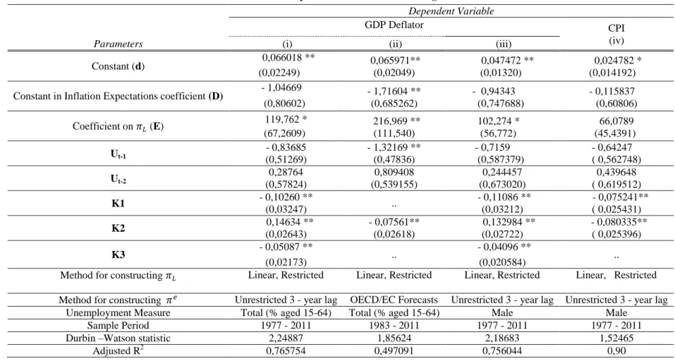
5.2. Portugal

In contrast with Germany, the estimation results for Portugal show that the ADP Phillips Curve fits best when GDP Deflator is used as a measure of inflation. Due to the small size of the Portuguese Economy, this fact may not come as a surprise as the CPI measurement is extremely prone to import inflation from its main trading partners. At first glance, the results here portrayed have a close resemblance with other empirical ADP Phillips Curves. Of particular interest is specification (ii), which uses the “Consensus Forecast” as a direct measure for , stands out for its good statistical fit, being the sole equation where lagged unemployment appears to be statistically significant. With this notable exception, the lack of efficiency in the estimates of unemployment is once more a drawback to our results, even though the sum of its coefficients is negative and similar with other countries.

Once more, the coefficient on inflation expectations bears good news for the ADP theory. While the statistical performance of is not exemplary, its estimates again imply less than complete incorporation of inflation in expectations. Similarly, is positive and significant in 3 of the 4 reported specifications (albeit mildly in specifications (i) and (iii)), thus confirming that the level of past inflation is still important in determining the degree of rational behavior.

When evaluating , we find that near rational behavior is especially salient in Portugal: save for (iv), the coefficient stands on average below 0,2 at zero inflation and full rationality is achieved only when inflation has reached double digit values of 14 percent. These results are somehow similar with Maugeri (2010) and, despite attesting

(40)

33 the existence of a (very) Long Run trade-off, the high inflation it may incurs is reason enough to cast some skepticism over the viability of exploring it without incurring serious consequences for the economy.

6. Conclusions and future research

In this dissertation, we sought to explore the subject of the unemployment - inflation relationship as defined by the Phillips Curve. Since its introduction, it has undergone a fierce debate surrounding the validity of its tenets and its functional form has been subject to considerable extensions throughout time. We have taken opportunity to review the main topics of the debate and to focus on the recent developments presented in Akerlof, Dickens and Perry (2000), who argue that the existence of near rational agents who incompletely incorporate inflation in expectations generates a Long Run trade-off which could be exploited by policy in order to improve welfare. We then decided to empirically replicate their model to Portugal and Germany.

Using different combinations of annual data, the main findings suggest that there is evidence of near-rational expectations in the Phillips Curve for both countries. Past performance of inflation has an impact over the way expectations are incorporated in the wage price setting process, and this result in smaller coefficient of expectation when inflation is low, enabling a Long-Run trade-off between inflation and unemployment. Even though the lack of efficiency in the estimates of unemployment prevents us from deriving the steady state unemployment and inflation rates – a fact which can be explained for the small data sample used - , the estimates follow closely those already reported in the literature. Given the current moment where both countries are enjoying an environment of low time inflation a common Monetary Policy, one cannot rule out a window of opportunity to call for the pursuit of expansionary policies.

(41)

34 Further paths of research could be advanced, though, which might bring improvements to the model. Downward nominal wage rigidity seems to be quite relevant in price and wage setting in Europe and introducing this variable into an ADP Phillips Curve could add extra information to the Near Rational ADP. Extending the range of indicators to include, for instance, productivity measures and specifications for

which were excluded in this work would also be a good idea.

Regarding the future adherence of the model, only time and further experimentation will tell how it behaves. Studies that fit an ADP Phillips Curve with quarterly data are found to display more statistically significant estimates than those using annual data, so the former data frequency should be preferred.

A word of caution is also made regarding the model. As Blinder (2000) argues, the ADP model doesn’t take other costs of inflation into consideration. If we blindly push the trade-off to very high inflation ranges simply because the coefficient of expectations is inferior to unity, the consequences are surely to be catastrophic.

A worthy proposal would be following the suggestion made in Lundborg & Sacklén (2006) and to check whether the Lowest Sustainable Unemployment Rate fulfills other objectives, such as maximum Output.

Near-rational expectations and the Phillips Curve : an empirical application

M

ESTRADO

ECONOMIA MONETÁRIA E FINANCEIRA

T

RABALHO

F

INAL DE

M

ESTRADO

DISSERTAÇÃO

N

EAR

-R

ATIONAL

E

XPECTATIONS AND THE

P

HILLIPS

C

URVE

:

AN

EMPIRICAL APPLICATION

J

OÃO MIGUEL CASANOVA NABAIS

M

ESTRADO EM

ECONOMIA MONETÁRIA E FINANCEIRA

T

RABALHO

F

INAL DE

M

ESTRADO

D

ISSERTAÇÃO

N

EAR

-R

ATIONAL

E

XPECTATIONS AND THE

P

HILLIPS

C

URVE

:

AN

EMPIRICAL APPLICATION

J

OÃO MIGUEL CASANOVA NABAIS

ORIENTAÇÃO:

MARGARIDA PAULA CALADO NECA VIEIRA DE ABREU

ISABEL MARIA DIAS PROENÇA

JÚRI:

Presidente: ANTÓNIO MANUEL PEDRO AFONSO

VOGAIS: EMANUEL GASTEIGER

Contents

2. The Phillips Curve Debate

4. The Akerlof-Dickens-Perry Model