CLUSTERING AN INTERVAL DATA SET
*1Áurea Sousa,
2Helena Bacelar
1
Department of Mathematics and CEEpl
2Faculty of Psychology and
3
Department of Mathematics, FCT, New Uni
4
Department of Mathematics and CICS.NOVA.UAc, University of Azores, Ponta Delgada,
ARTICLE INFO ABSTRACT In this paper we co
Ascendant Hierarchical Cluster Analysis (AHCA) symbolic data analysis (“
panel of human observers.
equal weights, and on the probabilistic coeffic
standardized weighted generalized affinity coefficient by the method of Wald and Wolfowitz. These similarity coefficients between elements were combined with three aggregation criteria, one
Single Linkage VL methodology
underlying data was carried out using some validation measures based on the similarity matrices. In general, global satisfactory results have been obtained using our meth
quite close (or even coinciding) with the
Copyright © 2015 Áurea Sousa et al. This is an open access article distributed under the Creative Commons Att distribution, and reproduction in any medium, provided the original work is properly cited.
INTRODUCTION
With the computational progress and the increased use of large data sets that on occasion require to be aggregated into smaller more manageable data sizes we need more complex data tables sometimes called “symbolic data tables”, where correspond to data units (frequently, groups of individuals, considered as second-order objects) and columns to variables In a table of this nature, each entry can contain just one value or several values, such as subsets of categories,
real data set, or frequency distributions (
2000; Bacelar-Nicolau, 2000, 2002; Diday and Noirhomme Fraiture, 2008; Bacelar-Nicolau et al., 2009, 2010, 2014 2014b; Sousa et al., 2010, 2013a, 2013b, 2014
particular, if each cell of a symbolic data table contains an interval we deal with interval variables. In fact, the
valued data arise in several situations such as recording monthly interval temperatures at meteorological stations instance, considering a town w, temperature (
January means that the temperature of the town
*Corresponding author: Áurea Sousa,
Department of Mathematics and CEEplA, University of Azores, Ponta Delgada, Portugal.
ISSN: 0975-833X
Vol.
Article History:
Received 19th August, 2015
Received in revised form
25th September, 2015
Accepted 07th October, 2015
Published online 30th November,2015
Key words:
Hierarchical clustering, Symbolic data, Interval data, Weighted generalised affinity coefficient, Probabilistic aggregation criteria, VL Methodology, Validations measures.
Citation:Áurea Sousa, Helena Bacelar-Nicolau, Fernando C. Nicolau and Osvaldo Silva main partitions similar to a priori partition?”, International Journal of Current Research
RESEARCH ARTICLE
CLUSTERING AN INTERVAL DATA SET – ARE THE MAIN PARTITIONS SIMILAR
TO A PRIORI PARTITION?
Bacelar-Nicolau,
3Fernando C. Nicolau and
Department of Mathematics and CEEplA, University of Azores, Ponta Delgada,
Faculty of Psychology and ISAMB, University of Lisbon, Lisbon, Portugal
Department of Mathematics, FCT, New University of Lisbon, Caparica,
Department of Mathematics and CICS.NOVA.UAc, University of Azores, Ponta Delgada,
ABSTRACT
In this paper we compare the best partitions of data units (cities) obtained from different algorithms of Ascendant Hierarchical Cluster Analysis (AHCA) of a well-known data set
symbolic data analysis (“city temperature interval data set”) with a priori
panel of human observers. The AHCA was based on the weighted generalised affinity, equal weights, and on the probabilistic coefficient, ( ,
standardized weighted generalized affinity coefficient by the method of Wald and Wolfowitz. These similarity coefficients between elements were combined with three aggregation criteria, one
gle Linkage (SL), and the other ones probabilistic, AV1 and AVB,
methodology. The evaluation of the partitions in order to find the partitioning that best fits the underlying data was carried out using some validation measures based on the similarity matrices. In general, global satisfactory results have been obtained using our meth
quite close (or even coinciding) with the a priori partition provided by the panel of human observers.
is an open access article distributed under the Creative Commons Attribution License, which distribution, and reproduction in any medium, provided the original work is properly cited.
With the computational progress and the increased use of large data sets that on occasion require to be aggregated into smaller more manageable data sizes we need more complex data tables sometimes called “symbolic data tables”, where rows correspond to data units (frequently, groups of individuals, order objects) and columns to variables.
each entry can contain just one value or several values, such as subsets of categories, intervals of the real data set, or frequency distributions (Bock and Diday, Nicolau, 2000, 2002; Diday and
Noirhomme-, 2009Noirhomme-, 2010Noirhomme-, 2014aNoirhomme-, , 2014, 2015). In f a symbolic data table contains an In fact, the interval-valued data arise in several situations such as recording monthly interval temperatures at meteorological stations (for erature (w)= [6, 12] in January means that the temperature of the town w varied in the
, University of Azores, Ponta
interval [6, 12] during the month of stock prices, etc. (De Carvalho
tables can also describe heterogeneous data and the values in their cells may be weighted and connected by logical rules and taxonomies (Bock and Diday, 2000).
data analysis methods (exploratory, graphical representations, cluster analysis, factorial analysis,…) to symbolic data tables is required.
Cluster analysis frequently appears in the literature under different names in different
unsupervised learning in pattern recognition, and taxonomy in biological sciences. The clustering aims at identifying and extract significant groups of elements to classify in the underlying data so that (based on a certain c
the elements in a cluster are more similar to each other than the elements in different clusters. Different types of algorithms to cluster analysis (e.g., partitional clustering, hierarchical clustering, density-based clustering, grid
been developed (Jain et al.
Hierarchical clustering proceeds successively
smaller clusters into larger ones (agglomerative methods), or by splitting larger clusters (divisive methods) (
International Journal of Current Research
Vol. 7, Issue, 11, pp.23151-23157, November, 2015
INTERNATIONAL
Nicolau, Fernando C. Nicolau and Osvaldo Silva, 2015. “Clustering an interval data set
International Journal of Current Research, 7, (11), 23151-23157
ARE THE MAIN PARTITIONS SIMILAR
and
4Osvaldo Silva
, University of Azores, Ponta Delgada, Portugal
ISAMB, University of Lisbon, Lisbon, Portugal
versity of Lisbon, Caparica, Portugal
Department of Mathematics and CICS.NOVA.UAc, University of Azores, Ponta Delgada, Portugal
obtained from different algorithms of known data set of the literature on
a priori partition of cities given by a
The AHCA was based on the weighted generalised affinity, ( , ′), with ( ′), associated with the asymptotic standardized weighted generalized affinity coefficient by the method of Wald and Wolfowitz. These similarity coefficients between elements were combined with three aggregation criteria, one classical,
AVB, the last ones in the scope of the
The evaluation of the partitions in order to find the partitioning that best fits the underlying data was carried out using some validation measures based on the similarity matrices. In general, global satisfactory results have been obtained using our methods, being the best partitions partition provided by the panel of human observers.
ribution License, which permits unrestricted use,
[6, 12] during the month of January), daily interval
et al., 2012). The symbolic data tables can also describe heterogeneous data and the values in may be weighted and connected by logical rules and
Diday, 2000). An extension of standard data analysis methods (exploratory, graphical representations, cluster analysis, factorial analysis,…) to symbolic data tables is
Cluster analysis frequently appears in the literature under contexts, such as for example unsupervised learning in pattern recognition, and taxonomy in biological sciences. The clustering aims at identifying and extract significant groups of elements to classify in the underlying data so that (based on a certain clustering criterion) the elements in a cluster are more similar to each other than the elements in different clusters. Different types of algorithms to cluster analysis (e.g., partitional clustering, hierarchical based clustering, grid-based clustering) have
et al., 1999; Lattin et al., 2003).
proceeds successively by either merging smaller clusters into larger ones (agglomerative methods), or by splitting larger clusters (divisive methods) (Halkidi et al.,
INTERNATIONAL JOURNAL OF CURRENT RESEARCH
Clustering an interval data set – are the 23157.
2001). Agglomerative methods usually start with each element to be classified in its own separate cluster. At each stage of the process, the most similar clusters (according to the selected aggregation criteria) are joined until only one cluster containing all elements remains. Given a set of n elements to classify, the divisive methods start with all elements in a single cluster and proceed dividing one cluster into two at each step until n clusters of size 1 remain. As is referred in Lattin et al. (2003) “Some methods are neither agglomerative nor divisive (e.g., various approaches that use least squares to fit certain tree structures)”. This paper is focused on agglomerative methods in the context of cluster analysis and on a symbolic data table where each cell contains an interval of the real axis. Some dissimilarity measures for interval data have been reported in
the literature (e.g., Chavent and Lechevallier, 2002; Chavent et al., 2003; Souza and De Carvalho, 2004; De Carvalho et al.,
2006a, 2006b, 2007), as well as some similarity measures which allow us to deal with this type of data (e.g., Guru et al., 2004; Bacelar-Nicolau et al., 2009, 2010, 2014a, 2014b; Sousa et al., 2010, 2013a, 2015).
A hierarchical algorithm allows us to obtain a tree of clusters, called dendrogram, which shows how the clusters are related. By cutting the dendrogram at an appropriate level, a partition of the elements to classify into disjoint groups is obtained. An important question is related to the number of clusters (How many clusters?). In fact, the evaluation of clustering results in order to find the partitioning that best fits the underlying data plays a very important role in cluster analysis (Halkidi et al., 2001).
Section 2 is devoted to the methods used to carry out the AHCA of cities, and to the measures of validation used to evaluate the obtained partitions. Section 3 is concerned to the main results obtained from the AHCA of the city temperature interval data set (issued from the symbolic data literature), and their comparison with a priori partition of cities given by a panel of human observers. The paper ends with some concluding remarks about the developed work.
Methodological framework
From the affinity coefficient between two discrete probability distributions proposed by Matusita (1951) as a similarity measure for comparing two distribution laws of the same type, Bacelar-Nicolau (e.g., 1980, 1988) introduced the affinity coefficient, as a similarity coefficient between pairs of variables or of subjects in cluster analysis context. After that, Bacelar-Nicolau extended that coefficient to different types of data, and the so-called weighted generalized affinity coefficient, ( , ′), between a pair of statistical data units, k and k’ (k, k’=1, …, N), is an extension of the affinity coefficient for the case of symbolic or complex data, which is able to deal with heterogeneous data (Bacelar-Nicolau, 2000, 2002; Bacelar-Nicolau et al., 2009, 2010, 2014a, 2014b).
Let = {1, ⋯ , } be a set of N data units described by p interval variables, Y1, …, Yp, which values are intervals of the
real data set (f. i., the entry (k, j), corresponding to the data unit k (k=1, …., N) and to the variable Yj ( j=1, …, p) of the data
table, contains an interval = , ). In this case, the
weighted generalized affinity coefficient, between a pair of statistical data units, k and k’ (k, k’=1, …,N), is defined in the following way: k'j kj k'j kj p j j
I
I
I
I
k
k
a
.
)
'
,
(
1
, (1)where π are weights such that 0 ≤ π ≤ 1, ∑ π = 1, and corresponds to a generalized Ochiai coefficient for interval data, associated with a 22 generalized contingency table which entries contain interval ranges instead of the usual cardinal numbers of any simple 22 contingency table (Bacelar-Nicolau et al., 2009, 2010, 2014b; Sousa et al., 2015). The formula (1) is a particular case of the general formula of the weighted generalized affinity coefficient when we are dealing with variables of interval type. In fact, the weighted generalized affinity coefficient between a pair of intervals may be computed in two different ways, either by using the general formula of the weighted generalized affinity coefficient considering the decomposition of the initial intervals into mj
elementary and disjoint intervals and working with the ranges of the elementary intervals; or, alternatively, by using the formula (1), without the decomposition of the initial intervals (for details, see Bacelar-Nicolau et al., 2009, 2010, 2014b).
Assuming a permutational reference hypothesis based on the limit theorem of Wald and Wolfowitz (Fraser, 1975), the random variable associated with
aff
I
kj,
I
k'j
has an asymptotic normal distribution. Two of the coefficients related with the ( , ′) coefficient, are the asymptotic standardized weighted generalized affinity coefficient, ( , ′), by the Wald and Wolfowitz method (see Bacelar-Nicolau, 1988; Bacelar-Nicolau et al., 2009, 2010, 2014a; Sousa et al., 2013a, 2015), and the associated probabilistic coefficient, ( , ′), in the scope of the VL methodology (V for Validity, L for Linkage), in the line started by Lerman (1970, 1972, 1981) and developed by Bacelar-Nicolau (e.g., 1980, 1985, 1987, 1988) and Nicolau (e.g., 1983, 1998). This last coefficient validates the affinity coefficient between two data units k, k' in a probabilistic scale (e.g., Bacelar-Nicolau, 1988, 2000; Bacelar-Nicolau et al., 2010; Lerman, 1972, 1981; Nicolau and Bacelar-Nicolau, 1998). The (hierarchical and non-hierarchical) clustering methods included in the VL-family are based on the cumulative distribution function of basic similarity coefficients (Bacelar-Nicolau, 1980, 1988; Nicolau, 1983; Nicolau and Bacelar-Nicolau, 1998).Here, we used the weighted generalized affinity coefficient, ( , ′), with equal weights ( = 1/ ), and the probabilistic coefficient, ( , ′), associated with the asymptotic standardized weighted generalized affinity coefficient by the method of Wald and Wolfowitz. In the case of the data set under analysis (“city temperature interval data set”) the best clustering results were provided by the probabilistic coefficient, ( , ′), as a consequence of standardizing the affinity values, and of using the corresponding probabilistic scale values. Thus, in the next section, a special emphasis will be given to the results provided
by the ( , ′) coef icient. A brief reference to the results obtained from the ( , ′) coefficient will be added. In order to compute these coefficients (similarity measures), we consider a previous decomposition of each interval of the original symbolic data table into a suitable number mj of elementary and
disjoint intervals, ℓ: ℓ = 1, ⋯ , (Bacelar-Nicolau et al.,
2009, 2010, 2014b). In this paper, the measures of comparison
between elements were combined with three aggregation criteria, one classical, Single Linkage (SL) or nearest neighbour method, and two probabilistic, AV1 and AVB, the last ones in the scope of the VL methodology, that use probabilistic notions for the definition of the comparative functions (e.g., Lerman, 1972, 1981, 2000; Nicolau, 1983; Bacelar-Nicolau, 1988; Nicolau and Bacelar-Nicolau, 1998).
An important step in cluster analysis is to determine the best number of clusters. In an optimal clustering scheme, the elements of each cluster should be as close to each other elements belonging to their cluster as possible (compactness), and the clusters should be widely spaced (isolation or separation). Therefore, is useful to use, for a cluster of elements, measures of its heterogeneity or lack of cohesion, and of its isolation or separation, from the rest of the data. These measures can be combined to provide measures of the adequacy of the partitions (Gordon, 1999). In fact, a general approach to finding the best partition involves defining a measure of the adequacy of a partition and seeking a partition of elements which optimizes that measure (Gordon, 1999).
Some measures of the heterogeneity of a cluster are defined in the literature (e.g., Gordon, 1999). Hennig (2005) refers to some different approaches that address different aspects of the validation problem, namely, use of external information (information that has not been used to generate the clustering), significance tests for clustering structure, comparison of different clustering structures on the same data set, validation indexes, stability assessment, and visual inspection. A global approach for evaluating the quality of clustering results provided from different clustering algorithms using the relevant information available (e.g., the stability, isolation and homogeneity of the clusters) was presented in Silva et al. (2012).
We used the methodological framework, described in Sousa et al. (2014), in order to evaluate the obtained partitions
according to measures of validation (adapted for the case of similarity measures) based on the values of the proximity matrix between elements (internal validation measures). Thus, the values of the statistics of levels STAT and DIF (Bacelar-Nicolau, 1980; Lerman, 1970, 1981), P(I2mod, ∑), and γ
(Goodman and Kruskal (1954)) indexes (for the partitions into three, four, and five clusters), were calculated. The "best" cluster is one that presents the largest values of STAT, DIF, and γ , and the smallest value of the P(I2mod, ∑). Furthermore, the values of the Sil* index based on the Silhouette plots (Rousseeuw, 1987) and of the U statistics (Mann and Whitney, 1947), namely the global U index (UG) and the local U index
(UL) were calculated for the clusters of the most significant
partition (according to the previous indexes), as described in
Sousa et al. (2014), and for the a priori partition. The formulae of the STAT, DIF, P(I2mod, ∑), and γ indexes, the last two ones adapted for the case of similarity measures, can be found in Sousa et al. (2013b). In the case of a cluster-L* we have UG=0 and in the case of a ball cluster we have UL=0 (Gordon,
1999). The best partition is compared with the a priori partition (external information) into four clusters given by a panel of human observers.
AHCA of the city temperature interval data set
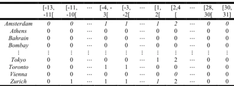
In this example, we consider the data set given in Guru et al. (2004) concerned to the minimum and the maximum monthly temperatures of 37 cities in degrees centigrade (city temperature interval data set) during a determined year. Table 1 shows a part of this data matrix.
The city temperature interval data set was given to a panel of human observers for classification. The a priori partition of the cities given by the observers contains four clusters (Guru et al., 2004), which descriptions and corresponding latitudes are shown in Table 2: Cluster 1: {C2, C3, C4, C5, C6, C8, C11, C12, C15, C17, C19, C22, C23, C29, C31}; Cluster 2: {C0, C1, C7, C9, C10, C13, C14, C16, C20, C21, C24, C25, C26, C27, C28, C30, C33, C34, C35, C36}; Cluster 3: {C18}; Cluster 4: {C32}.
The cities belonging to cluster 1 are located at latitudes between 0º and 40º and the cities included in the cluster 2 are mainly located at latitudes between 40º and 60 º. The human observers have classified some cities (C1- Athens, C13- Lisbon, C27- San Francisco, C28- Seoul and C33- Tokyo), which are closer to the sea coast and are located at latitudes between 0 and 40, in the cluster 2, because those cities have low
Table 1. Data matrix- Minimum and maximum temperatures of cities in centigrade degrees
Pattern no. Cities Jan. Feb. Mar. ⋯ Oct. Nov. Dec.
C0 Amsterdam [-4, 4] [-5, 3] [2, 12] ⋯ [5, 15] [1, 10] [-1, 4] C1 Athens [6, 12] [6, 12] [8, 16] ⋯ [16, 23] [11, 18] [8, 14] C2 Bahrain [13, 19] [14, 19] [17, 23] ⋯ [24, 31] [20, 26] [15, 21] C3 Bombay [19, 28] [19, 28] [22, 30] ⋯ [24, 32] [23, 32] [20, 30] ⋮ ⋮ ⋮ ⋮ ⋮ ⋮ ⋮ ⋮ ⋮ C33 Tokyo [0, 9] [0, 10] [3, 13] ⋯ [13, 21] [8, 16] [2, 12] C34 Toronto [-8, -1] [-8, -1] [-4, 4] ⋯ [6, 14] [-1, 17] [-5, 1] C35 Vienna [-2, 1] [-1, 3] [1, 8] ⋯ [7, 13] [2, 7] [1, 3] C36 Zurich [-11, 9] [-8, 15] [-7, 18] ⋯ [3, 22] [0, 19] [-11, 8]
temperature which is similar to that of the cities which are located at latitudes between 40 and 60. “The cities nearer to sea coast bear relatively low temperature because of the cool breeze from the sea coast and also due to high humidity present in the atmosphere” (Guru et al., 2004). Mauritius (the only island in this data set) was included in a cluster with only one element (singleton) and Tehran in other singleton due to its irregular temperature. The main results of the hierarchical cluster analysis of the 37 cities are presented in the remaining section.
Table 2. Description of a priori partition - city temperature interval data set
Cluster 1 Latitude Cluster 2 Latitude
C2-Bahrain 26°13'N C0-Amsterdam 52°22'N C3-Bombay 19°0'N C1-Athens 37°58'N C4-Cairo 30°3'N C7-Copenhagen 55°41'N C5-Calcutta 22°34'N C9-Frankfurt 50°07'N C6-Colombo 6°56'N C10-Geneva 46°12'N C8-Dubai 25°15'N C13-Lisbon 38°43'N
C11- Hong Kong 22°17'N C14-London 51°30'N
C12- Kuala Lampur 3°8'N C16-Madrid 40°24'N
C15- Madras 13°05'N C20-Moscow 55°45'N
C17-Manila 14°35'N C21-Munich 48°08'N
C19-Mexico 19°26'N C24-New York 42°54'N
C22-Nairobi 1°17'S C25-Paris 48°51'N
C23-New Delhi 28°37'N C26-Rome 41°54'N
C29 - Singapore 1°17'N C27-San Francisco 37°47'N
C31-Sydney 33°52'S C28-Seoul 37°34'N --- --- C30-Stockholm 59°20'N --- --- C33-Tokyo 35°41'N --- --- C34-Toronto 43°42'N --- --- C35-Vienna 48°13'N --- --- C36-Zurich 47°22'N
Cluster 3 Latitude Cluster 4 Latitude
C18-Mauritius 20°10'S C32-Tehran 35°42'N
Before calculating the values of the ( , ′) and ( , ′) coefficients, the domains of each variable Yj, j=1,…,12, for
the set E={1, …, 37} of n=37 objects (cities) were decomposed into a suitable number of elementary and disjoint intervals. For instance, the observed (interval-type) values of V1 (January)
are V1(E): {[-4, 4]; [6, 12]; [13, 19]; [19, 28]; [8, 20]; [13, 27];
[22, 30]; [-2, 2]; [13, 23]; [-10, 9]; [-3, 5]; [13, 17]; [22, 31]; [8, 13]; [2, 6]; [20, 30]; [1, 9]; [21, 27]; [22, 28]; [6, 22]; [-13, -6]; [-6, 1]; [12, 25]; [6, 21]; [-2, 4]; [1, 7]; [4, 11]; [6, 13]; [0, 7]; [23, 30]; [-9, -5]; [20, 30]; [0, 5]; [0, 9]; [-8, -1]; [-2, 1]; [-11, 9]}. Thus, the domain of variable V1 is the interval = [-13,
31]. Let u0= -13, u1= -11, u2= -10, u3=-9, u4=-8, u5= -6, u6= -5,
u7=-4, u8= -3, u9=-2, u10= -1, u11=0, u12=1, u13=2, u14=4, u15=5,
u16=6, u17=7, u18=8, u19=9, u20=11, u21=12, u22=13, u23=17,
u24=19, u25=20, u26=21, u27=22, u28=23, u29=25, u30=27, u31=28,
u32=30, and u33=31 be the 34 distinct values corresponding to
the lower and upper boundaries of the observed intervals of V1(E) that are sorted in ascending order. The interval is
decomposed into 33 elementary and disjoint intervals, ,, ( = 1, ⋯ ,33) based on the 34 distinct values, u0,
…, u33, as follows:
[13, 11[; [11, 10[; [10, 9[; [9, 8[; [8, 6[; [6, 5[; [5, -4[; [-4, -3[; [-3, -2[; [-2, -1[; [-1, 0[; [0, 1[; [1, 2[; [2, -4[; [4, 5[; [5, 6[; [6, 7[; [7, 8[; [8, 9[; [9, 11[; [11, 12[; [12, 13[; [13, 17[; [17, 19[; [19, 20[; [20, 21[; [21, 22[; [22, 23[; [23, 25[; [25, 27[; [27, 28[; [28, 30[; [30, 31] (see Table 1). For example,
still in the case of V1 (January), the intervals concerning,
respectively, to the cities Amsterdam and Athens are the following (see Table 3, which entries are ranges of the elementary intervals):
Aj=[-4, 4]=[-4, -3[[-3, -2[ [-2, -1[ [-1, 0[ [0, 1[ [1, 2[ [2, 4];
Bj= [6, 12]= [6, 7[ [7, 8[[8, 9[ [9, 11[ [11, 12].
Therefore, proceeding in this way for all other variables, we obtained a new data matrix, subdivided into 12 subtables (one for each variable), which contain a decomposition of the respective initial intervals into elementary intervals.
Table 3. Decomposition into 33 elementary intervals – Variable Y1
(January) [-13, -11[ [-11, -10[ ⋯ [4, -3[ [-3, -2[ ⋯ [1, 2[ [2,4 [ ⋯ [28, 30[ [30, 31] Amsterdam 0 0 ⋯ 1 1 ⋯ 1 2 ⋯ 0 0 Athens 0 0 ⋯ 0 0 ⋯ 0 0 ⋯ 0 0 Bahrain 0 0 ⋯ 0 0 ⋯ 0 0 ⋯ 0 0 Bombay 0 0 ⋯ 0 0 ⋯ 0 0 ⋯ 0 0 ⋮ ⋮ ⋮ ⋮ ⋮ ⋮ ⋮ ⋮ ⋮ ⋮ ⋮ ⋮ Tokyo 0 0 ⋯ 0 0 ⋯ 1 2 ⋯ 0 0 Toronto 0 0 ⋯ 1 1 ⋯ 0 0 ⋯ 0 0 Vienna 0 0 ⋯ 0 0 ⋯ 0 0 ⋯ 0 0 Zurich 0 1 ⋯ 1 1 ⋯ 1 2 ⋯ 0 0
Table 4 contains the partitions into three, four, and five clusters provided by the probabilistic similarity coefficient, ( , ′), combined with the three aggregation criteria (SL, AV1, and AVB).
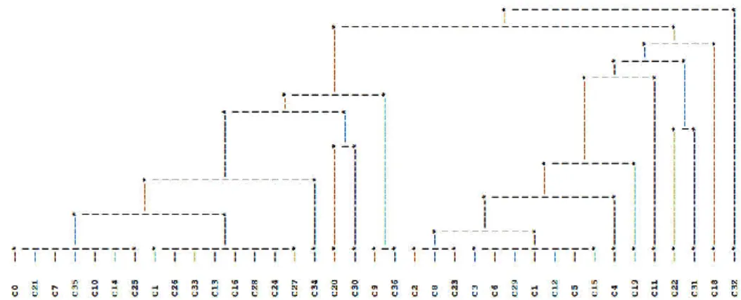
In the case of the probabilistic similarity coefficient, ( , ′), the partition into four clusters of the dendrogram obtained from the SL method (see Table 4 and Figure 1) is
identical to that provided by the panel of human observers (a priori partition). This partition was also obtained by Guru et al. (2004), using a similarity measure for estimating the degree of similarity among patterns (described by interval type data) in terms of multivalued data, and un unconventional agglomerative clustering technique, by introducing the concept of mutual similarity value (Guru et al., 2004). The partition into four clusters provided by the AV1 and AVB methods (see Table 4 and Figure 2) it is not the same that the a priori partition (others authors (e.g., De Carvalho, 2007)
also have obtained partitions into four clusters that were not identical to that a priori partition). It can be seen that the partition into three clusters provided by the ( , ′) coefficient combined with the three applied aggregation criteria is quite close to the a priori partition given by the panel of human observers, excepting in what concerns the location of city 18, which in the classification given by the panel of human observers is a cluster with only one element (singleton) [see Figures 1 and 2]. This is also the most significant partition (the best partition), according to all applied validation indexes, as is shown in Table 5, due to the maximum values of STAT (18.9912), DIF (2.3429) in the case of AV1 and AVB), and (0.8524), and to the minimum value (0.3176) of P(I2mod,). Cluster 1: {C0, C1, C7, C9, C10, C13, C14, C16, C20, C21, C24, C25, C26, C27, C28, C30, C33, C34, C35, C36}; Cluster 2: {C32}; Cluster 3: {C2, C3, C8, C4, C5, C6, C11, C12, C15, C17, C18, C19, C22, C23, C29, C31}.
That partition was also the best partition according to the STAT (18.6694), DIF (0.4982), and P(I2mod,) (0.1282) indexes obtained from the ( , ′) coefficient combined with the AV1 and AVB methods.
The partition into four clusters provided by the ( , ′) coefficient combined with the SL method is identical to the a priori partition (the same is not verified in the case of the application of the ( , ′) coefficient combined with the SL method).
Figure 1. Dendrogram obtained by the probabilistic coefficient, ( , ′), + SL method (last levels)
Figure 2. Dendrogram obtained by the probabilistic coefficient, ( , ′),+ AV1 method (last levels)
Table 4. Partitions into three, four and five clusters - ( , ′)
Number of clusters
Methods Cluster 1 Cluster 2 Cluster 3 Cluster 4 Cluster 5
3 ( , ′)+ SL ( , ′)+AV1 ( , ′)+ AVB C2, C3, C4, C5, C6, C8, C11, C12, C15, C17, C18, C19, C22, C23, C29, C31 C0, C1, C7, C9, C10, C13, C14, C16, C20, C21, C24, C25, C26, C27, C28, C30, C33, C34, C35, C36 C32 4 ( , ′)+ SL C2, C3, C4, C5, C6, C8, C11, C12, C15, C17, C19, C22, C23, C29, C31 C0, C1, C7, C9, C10, C13, C14, C16, C20, C21, C24, C25, C26, C27, C28, C30, C33, C34, C35, C36 C18 C32 ( , ′)+AV1 ( , ′)+ AVB C0, C7, C10, C14, C20, C21, C25, C30, C34, C35 C1, C9, C13, C16, C24, C26, C27, C28, C33, C36 C2, C3, C4, C5, C6, C8, C11, C12, C15, C17, C18, C19, C22, C23, C31, C29 C32 5 ( , ′)+ SL C0, C1, C7, C9, C10, C13, C14, C16, C20, C21, C24, C25, C26, C27, C28, C30, C33, C34, C35, C36 C2, C3, C4, C5, C6, C8, C11, C12, C15, C17, C19, C23, C29 C22, C31 C18 C32 ( , ′)+AV1 ( , ′)+ AVB C0, C7, C10, C14, C20, C21, C25, C30, C34, C35 C3, C5, C6, C12, C15, C17, C29 C1, C9, C13, C16, C24, C26, C27, C28, C33, C36 C32 C2, C4, C8, C11, C18, C19, C22, C23, C31
Table 5. Values of validation measures for the partitions into three, four, and five clusters
STAT DIF P(I2mod, )
SL AV1/AVB SL AV1 AVB SL AV1/AVB SL AV1/AVB
5 Clusters 18.5947 15.7538 0.6431 0.7185 0.1887 .3871 .3875 .8484 .8504
4 Clusters 18.3947 16.6483 -0,2 0.8945 0.8945 .3694 .3700 .8291 .8022
The values of Sil* and of U statistics (UL/UG) for the cluster 2
belonging to the partition in to three clusters and to the a priori partition are, respectively, 0.5270 and 569/4782. Moreover, the cluster 1 belonging to the partition into three clusters has a higher value of Sil*, and a lower value of U statistics (UL / UG)
compared to the corresponding ones of the cluster 1 of the partition provided by the human observers (Sil*=0.4917; UL/UG
= 423/2598 versus Sil*=0.4897; UL/UG = 474/2687). According
with the U statistics of Mann and Whitney (Gordon, 1999), the clusters concerning to the partitions into three and to the a priori partition into four clusters, with more than one element, are neither ball clusters nor l*-clusters, however they are dense and well separated clusters, because they present relatively high values of the Sil* index. The "best" cluster is one that presents the largest value of Sil* and the smallest value of the U statistics (UL and UG). Thus, the best partition (into
three clusters), according to the applied validation measures, is also slightly better than the partition into four clusters provided by the human panel.
Conclusion
The city temperature interval data set, as well as other experiments with different real and artificial interval data sets, have shown the usefulness of the weighted generalised affinity, ( , ′), and of two related coefficients, namely, the asymptotic standardized weighted generalized affinity coefficient by the method of Wald and Wolfowitz, ( , ′), and the associated probabilistic coefficient, ( , ′). The use of the probabilistic coefficient, ( , ′), instead of the coefficient ( , ′), allows us to work with comparable similarity values in a probabilistic scale. Moreover, the used validation measures are helpful in the selection of the best partitions of the elements to be classified.
Global satisfactory results were obtained using our approach, and one of the obtained partitions is in complete accordance with the partition into four clusters provided by the panel of human observers (a priori partition), although it is not the best one, according to the applied validation measures. The validation measures point to the partition into three clusters as the best partition.
REFERENCES
Bacelar-Nicolau, H. 1980. Contributions to the study of comparison coefficients in cluster analysis, Ph.D Thesis (in Portuguese), Universidade de Lisboa, Portugal.
Bacelar-Nicolau, H. 1985. "The affinity coefficient in cluster analysis", Methods of Operations Research, vol. 53, M. J. Beckmann, K.-W. Gaede, K. Ritter, & H. Schneeweiss (Eds.), Verlag Anton Hain, Munchen, pp. 507-512.
Bacelar-Nicolau, H. 1987. “On the distribution equivalence in cluster analysis”. In Devijver, P.A. & Kittler, J. (Eds.) Pattern Recognition Theory and Applications, NATO ASI Series, Series F: Computer and Systems Sciences, vol. 30, Springer - Verlag, New York, pp. 73-79.
Bacelar-Nicolau, H. 1988. “Two probabilistic models for classification of variables in frequency tables”. In: Bock, H.-H. (Eds.), Classification and related methods of data analysis, Elsevier Sciences Publishers B.V., North Holland, pp. 181-186.
Bacelar-Nicolau, H. 2000. “The affinity coefficient”. In: Analysis of symbolic data: Exploratory methods for extracting statistical information from complex data, H.-H. Bock & E. Diday (Eds.), Series: Studies in Classification, Data Analysis, and Knowledge Organization, Springer-Verlag, Berlin, pp. 160-165.
Bacelar-Nicolau, H. 2002. “On the generalised affinity coefficient for complex data”, Biocybernetics and Biomedical Engineering, vol. 22, no. 1, pp. 31-42.
Nicolau, H., Nicolau, F.C., Sousa, Á., & Bacelar-Nicolau, L. 2009. “Measuring similarity of complex and heterogeneous data in clustering of large data sets”, Biocybernetics and Biomedical Engineering, vol. 29, no. 2, pp. 9-18.
Nicolau, H., Nicolau, F.C., Sousa, Á., & Bacelar-Nicolau, L. 2010. “Clustering complex heterogeneous data using a probabilistic approach”, Proceedings of the Stochastic Modeling Techniques and Data Analysis International Conference (SMTDA2010), pp. 85-93. Nicolau, H., Nicolau, F.C., Sousa, Á., &
Bacelar-Nicolau, L. 2014a. “Clustering of variables with a three-way approach for health sciences”, Testing, Psychometrics, Methodology in Applied Psychology (TPM), vol. 21, no. 4, pp. 435-447.
Nicolau, H., Nicolau, F.C., Sousa, Á., & Bacelar-Nicolau, L. 2014b. “On cluster analysis of complex and heterogeneous data”, Proceedings of the 3rd Stochastic Modeling Techniques and Data Analysis International Conference (SMTDA2014), C. H. Skiadas (Eds.), 2014 ISAST, pp. 99-108.
Bock, H.-H., & Diday, E. (Eds.) 2000. Analysis of symbolic data: Exploratory methods for extracting statistical information from complex data, Series: Studies in Classification, Data Analysis, and Knowledge Organization, Springer-Verlag, Berlin.
Chavent, M. & Lechevallier, Y. 2002. “Dynamical clustering algorithm of interval data: Optimization of an adequacy criterion based on Hausdorff distance”. In Classification, clustering, and data analysis, K. Jajuga, A. Sokolowski, H.-H. Bock (Eds.), Springer-Verlag, Berlin, pp. 53-60.
Chavent, M., De Carvalho, F.A.T., Lechevallier, Y., & Verde, R. 2003. “Trois nouvelles méthodes de classification automatique de données symboliques de type intervalle”, Revue de Statistique Appliquée, vol. LI, no. 4, pp. 5-29. De Carvalho, F.A.T., Bertrand, P. & Melo, F. 2012. “Batch
self-organizing based on city-block distances for interval variables”. 15 pages<hal-00706519>
De Carvalho, F. A. T., Brito, P. & Bock, H.-H. 2006a. “Dynamic clustering for interval data based on L2 distance”, Computational Statistics, vol. 21, no. 2, pp. 1-19. De Carvalho, F.A.T., Souza, R.M.C.R. de, Chavent, M., &
Lechevallier, Y. 2006b. “Adaptive Hausdorff distances and dynamic clustering of symbolic interval data”, Pattern Recognition Letters, vol. 27, no. 3, pp. 167-179.
De Carvalho, F.d.A.T. 2007. “Fuzzy c-means clustering methods for symbolic interval data”, Pattern Recognition Letters, vol. 28, no. 4, pp. 423-437.
Diday, E., & Noirhomme-Fraiture, M. (Eds.) 2008. Symbolic data analysis and the SODAS software, John Wiley & Sons, Chichester.
Goodman, L. A., & Kruskal, W.H. 1954. “Measures of association for cross-classifications”, Journal of the American Statistical Association, 49, pp. 732-64.
Gordon, A.D. 1999. Classification, 2nd ed., London: Chapman & Hall.
Guru, D. S., Kiranagi, Bapu B., & Nagabhushan, P. 2004. “Multivalued type proximity measure and concept of mutual similarity value useful for clustering symbolic patterns”. Pattern Recognition Letters, vol. 25, no. 10, pp. 1203-1213.
Halkidi, M., Batistakis, Y., & Vazirgiannis, M. 2001. “On clustering validation techniques”, Journal of Intelligent Information Systems, 17:2/3, pp. 107–145.
Hennig, C. 2005. “A method for visual cluster validation”. In C. Weihs and W. Gaul (Eds.), Classification - The Ubiquitous Challenge, pp. 153–160, Springer, Berlin. Jain, A.K., Murty, M.N., & Flynn, P.J. 1999. “Data clustering:
Areview”, ACM Computing Surveys, vol. 31, no. 3, pp. 264-323.
Lattin, J., Carrol J.D., & Green, P.E. 2003. Analysing multivariate data. Duxbury applied series, Thomson Brooks/Cole.
Lerman, I.C. 1970. “Sur l`analyse des donnéespréalable àun classification automatique (Proposition d’une nouvelle mesure de similarité)”, Rev. Mathémati queset Sciences Humaines, vol. 32, no. 8, pp. 5-15.
Lerman, I.C. 1972. Étude distributionelle de statistiques de proximité entre structures algébriquesfinies dumême type: Apllication à la classification automatique, Cahiers du B.U.R.O., 19, Paris.
Lerman, I.C. 1981. Classification et analyse ordinale des données, Dunod, Paris.
Lerman, I.C. 2000. “Comparing taxonomy data”. Revue Mathematiqueset Sciences Humaines, 38, pp. 37-51. Mann, H., & Whitney, D. 1947. “On a test of whether One of
two random variables is stochastically larger than the other”, Annals of Mathematical Statistics, 18, pp. 50-60, 1947.
Matusita, K. 1951. “On the theory of statistical decision functions”, Annals of the Institute of Statistical Mathemathics, vol. 3, pp. 17-35.
Nicolau, F.C. 1983. “Cluster analysis and distribution function”, Methods of Operations Research, vol. 45, pp. 431-433.
Nicolau, F.C., & Bacelar-Nicolau, H. 1998. ”Some trends in the classification of variables”. In: Hayashi, C., Ohsumi, N., Yajima, K., Tanaka, Y., Bock, H.-H., & Baba, Y. (Eds.), Data Science, Classification, and Related Methods, Springer-Verlag, pp. 89-98.
Rousseeuw, P.J. 1987. “Silhouettes: A graphical aid to the interpretation and validation of cluster analysis”, Journal of Computational and Applied Mathematics, 20, pp. 53-65. Silva, O., Bacelar-Nicolau, H. & Nicolau, F.C. 2012. “A global
approach to the comparison of clustering results”, Biometrical Letters, vol. 49, no. 2, pp. 135-147.
Sousa, Á., Bacelar-Nicolau, H., Nicolau, F.C., & Silva, O. 2015. "On clustering interval data with different scales of measures: Experimental results", Asian Journal of Applied Science and Engineering, vol. 4, pp. 17-25, 2015.
Sousa, Á., Nicolau, F. C., Bacelar-Nicolau, H., & Silva, O. 2010. “Weighted generalised affinity coefficient in cluster analysis of complex data of the interval type”, Biometrical Letters, vol. 47, no. 1, pp. 45-56.
Sousa, Á., Nicolau, F.C., Bacelar-Nicolau, H., & Silva, O. 2013a. “Clustering of symbolic data based on affinity coefficient: Application to a real data set”, Biometrical Letters, vol. 50, no. 1, pp. 27-38.
Sousa, Á., Tomás, L., Silva, O., & Bacelar-Nicolau, H. 2013b. “Symbolic data analysis for the assessment of user satisfaction: An application to reading rooms services”. Proceedings of the First Annual International Interdisciplinary Conference, AIIC 2013, 24-26 April, Portugal, pp. 39-48, European Scientific Journal (ESJ) June 2013/Special/ Edition nº 3.
Sousa, Á., Nicolau, F.C, Bacelar-Nicolau, H., & Silva, O. 2014. "Cluster analysis using affinity coefficient in order to identify religious beliefs profiles", European Scientific Journal (ESJ), vol. 3 (Special edition), pp. 252 - 261. Souza, R.M.C.R., & De Carvalho, F.A.T. 2004. “Clustering of
interval data based on City-Block distances”, Pattern Recognition Letters, vol. 25, pp. 353-365.
Souza, R.M.C.R., De Carvalho, F.A.T., & Pizzato, D.F. 2007. “A partitioning method for mixed feature-type symbolic data using a squared Euclidean distance”. IN FREKSA, C., KOHLHASE, M., & SCHILL, K. (Eds.) KI 2006: Advances in artificial intelligence. 29th Annual German Conference on AI, KI 2006, Bremen, Germany, June 14-17, 2006, Proceedings. Series: Lecture notes in computer science, vol. 4314, Springer-Verlag, Berlin Heidelberg, pp. 260-273.