M
ASTER OF
S
CIENCE IN
FINANCE
M
ASTERS
F
INAL
W
ORK
D
ISSERTATION
D
ID THE
R
ECENT
F
INANCIAL
C
RISIS
C
ONTRIBUTE TO
A
N
EU
M
ULTI
-S
PEED
B
ANKING
S
YSTEM
?
J
OÃO
C
ARLOS
M
ARQUES
T
OMÁS
G
RADE
M
ONTEIRO
M
ASTER OF
S
CIENCE IN
FINANCE
M
ASTERS
F
INAL
W
ORK
D
ISSERTATION
D
ID THE
R
ECENT
F
INANCIAL
C
RISIS
C
ONTRIBUTE TO
A
N
EU
M
ULTI
-S
PEED
B
ANKING
S
YSTEM
?
J
OÃO
C
ARLOS
M
ARQUES
T
OMÁS
G
RADE
M
ONTEIRO
S
UPERVISOR
P
ROFª
D
OUTORA
M
ARIA
C
ÂNDIDA
R
ODRIGUES
F
ERREIRA
i
Resumo
O elevado impacto da crise financeira de 2007-08 na União Europeia (UE) gerou um período marcado por incerteza e ineficiência, enfatizando as discrepâncias entre os países pertencentes à UE.
A presente dissertação tem como principal propósito investigar os efeitos da recente crise financeira no desempenho do sistema bancário em diferentes países da UE, apresentando resultados empíricos da sua evolução durante o período de 2000 a 2014. Um painel composto por 12 países pertencentes à UE (Alemanha, Áustria, Bélgica, Espanha, França, Holanda, Grécia, Irlanda, Itália, Portugal, Reino Unido e Suécia) foi selecionado e subdividido de acordo com a reacção dos países face à crise financeira. Foram analisados três níveis de eficiência (Eficiência Técnica, Alocativa e de Custos) obtidos através da metodologia Data Envelopment Analysis, um método não paramétrico, usando como variáveis os dados presentes nas contas consolidadas das demonstrações financeiras do aglomerado de bancos comerciais e de poupança de cada país, obtidos através da base de dados Bankscope.
Os principais resultados da análise indicam um aumento dos níveis de eficiência nos países analisados da UE nos últimos anos, bem como a redução das oscilações dos níveis de eficiência. A comparação entre os países analisados permitiu concluir que se mantém um fosso nos níveis de eficiência no periodo Pós-Crise, induzindo diferentes impactos e reacções à crise financeira por parte dos países definidos para esta análise. No entanto não existe evidência empírica de uma relação entre indicadores macroeconómicos e eficiência bancária nos países selecionados.
Palavras–Chave: Crise Financeira; DEA; Desempenho Bancário; Eficiência de Custos; União Europeia.
ii
Abstract
The impact of the global financial crisis of 2007-08 in the European Union (EU) induced a transition process marked by uncertainty and inefficiency, emphasizing the discrepancies among EU countries.
Following this thought, this paper aims to investigate the effects of the recent financial crisis in bank system performance in different EU countries, providing empirical evidence regarding its evolution over the period of time 2000-2014. A panel composed of 12 EU countries (Austria, Belgium, France, Germany, Greece, Ireland, Italy, Netherlands, Portugal, Spain, Sweden and United Kingdom) was selected and subdivided according to countries’ reactions to the financial crisis. Three types of efficiency (Technical, Allocative and Cost
Efficiency) were computed applying the Data Envelopment Analysis, a non-parametric
approach, using as bank level variables the annual consolidated financial statement accounts of the agglomerate commercial and savings banks presented in BankScope Database.
The main results point out an overall improvement of banking efficiency in the EU in the last sample years as well as a reduction of efficiency level´s oscillations in a yearly basis. From the comparison of banking efficiency among the selected countries it was observed the maintenance of a significant efficiency level gap in the Post-Crisis period, inducing different impacts and reactions to periods of financial distress in the countries defined for this analysis. Nevertheless, it was not found any strong empirical evidence of a relationship between bank performance and macroeconomic environment in the selected countries.
iii
Acknowledgments
This dissertation is the final result of a long and hard journey as student at ISEG, an institution where I had the opportunity to grow personal and professionally. I want to express my sincere gratitude to those who accompanied me during this journey.
To Prof. Maria Cândida Rodrigues Ferreira for her kind support, availability and critical view along the months involving the elaboration of the present dissertation.
To all my friends, colleagues and professors at ISEG, for their friendship and support during these years.
To all my family for their unconditional support and encouragement in all moments of my life.
iv
Table of Contents
Resumo ...i
Abstract ... ii
Acknowledgments ... iii
Index of Figures ... v
Index of Figures in Appendix ... v
Index of Tables ... v
Index of Tables in Appendix ... vi
Index of Abbreviations ... vii
1.
Introduction ... 1
2.
Efficiency Frontier Approach ... 4
3.
Literature Review ... 6
4.
Methodology and Data ... 9
4.1 Data Envelopment Analysis (DEA) ... 9
4.2 Data ...11
4.3 Input and Output Variables ...14
5.
Empirical Results ... 17
5.1 EU Banking Efficiency Evolution ...17
5.2 Cost Efficiency Results ...19
5.3 Technical and Allocative Efficiency Results ...25
6.
Conclusions ... 32
References ... 35
Appendix ... 39
Appendix A. Farrell Efficiency ...40
Appendix B. Literature Review ...41
Appendix C. Macroeconomic Environment in EU ...42
Appendix D. Bank Level Data ...44
v
Index of Figures
Figure 1. Evolution of Efficiency Levels over Time 17
Index of Figures in Appendix
Appendix A. Farrel Efficiency
Figure A 1. Farrell Frontier Efficiency
Appendix C. Macroeconomic Environment in EU
Figure C 1. Evolution of Real GDP Growth Rate in the EU – 28 Countries (in p.p.) Figure C 2. Real GDP Growth Rate Evolution of Group A in Post Crisis Period Figure C 3. Real GDP Growth Rate Evolution of Group B in Post Crisis Period Figure C 4. Real GDP Growth Rate Evolution of Group C in Post Crisis Period
Appendix E. Efficiency Results
Figure E 1. Evolution of Average and Standard Deviation of Cost Efficiency
Index of Tables
Table 1. Groups and Countries used in Data Set 12
Table 2. Descriptive Statistics of Bank Level Variables 16
Table 3. Descriptive Statistics of Cost Efficiency Results 19
Table 4. Cost Efficiency Results 22
Table 5. Comparison of Cost Efficiency – Group A 23
Table 6. Comparison of Cost Efficiency – Group B 23
Table 7. Comparison of Cost Efficiency – Group C 24
Table 8. Technical and Allocative Efficiency 25
Table 9. Technical Efficiency Results 26
Table 10. Allocative Efficiency Results 27
Table 11. Comparison of Technical and Allocative Efficiency – Group A 29 Table 12. Comparison of Technical and Allocative Efficiency – Group B 29 Table 13. Comparison of Technical and Allocative Efficiency – Group C 30
40 42 42 42 42 53
vi
Index of Tables in Appendix
Appendix B. Literature Review
Table B 1. Resume Board of Cross Country EU Banking Efficiency Studies
Appendix C. Macroeconomic Environment in EU
Table C 1. Macroeconomic Pre and Post Crisis Comparison
Appendix D. Bank Level Data
Table D 1. Definition of Bank Variables among Efficiency Frontier Literature Table D 2. Total Loans (Output)
Table D 3. Other Earning Assets (Output) Table D 4. Other Operating Income (Output)
Table D 5. Deposits and Short Term Funding (Input) Table D 6. Other Interest Bearing Liabilities (Input) Table D 7. Loan Loss Provisions (Input)
Table D 8. Number of Commercial and Savings Banks
Appendix E. Efficiency Results
Table E 1. Overall Efficiency Comparison
Table E 2. Absolute and Cumulative Frequency of Efficiency Results by Quartiles
41 43 44 45 46 47 48 49 50 51 52 53
vii
Index of Abbreviations
AE – Allocative Efficiency CE – Cost Efficiency
DEA - Data Envelopment Analysis DFA - Deterministic Frontier Analysis DMU – Decision Making Unit
EC – European Commission ECB – European Central Bank EU – European Union
GDP – Gross Domestic Product HHI – Herfindahl-Hirschman Index IMF – International Monetary Fund M&A – Mergers and Acquisitions SFA – Stochastic Frontier Analysis TE – Technical Efficiency
TFA - Thick Frontier Analysis USA – United States of America
1
1. Introduction
The complexity of the financial crisis of 2007-08 derived a wide number of studies regarding the reasons, motives and impact in the global economy, particularly in the European Union (EU) economy as one of the most affected areas around the globe.
The financial crisis of 2007-08 initiated as a real state bubble in the United States of America (USA) was marked by the intensive risk involved on transactions, particularly due to facilities on the access to credit even for those without a collateral associated (the
subprime). The burst of the bubble in 2007 turned the USA economy into a distrust scenario
with the sudden rise of the risk aversion and the fall of the investment, which led to liquidations, strike-outs and unemployment. The financial crisis was globally spread, due to transmission mechanisms among worldwide economies and the solid linkages between financial institutions.
The European Union can be considered as the region where the financial crisis had higher impact, leading to a severe deceleration of EU economies’ growth (Figure C1). This can be explained, in part, by the liberalization and the deregulation processes on the banking sector in the 90´s. It increased the competition and imposed the diversification of banks portfolios with the widespread of more volatile financial instruments and sources of revenue (securitization). In addition it incentive the development of new business models, leading to changes on the Monetary Transmission Mechanism (Gambacorta and Marques-Ibanez (2011)).
The increase of securitization had, therefore, a significant impact on the crisis, since it induced a high impact on banks ‘performance in periods of distress, as referred by many authors namely, Altunbas et al. (2001); Lehmann and Nyberg (2014) and Pawlowska (2015), who referred that the growth of credit to private sector in the EU caused imbalances and boosted the heterogeneity of banking sector in the EU countries.
2
Some literature has devoted attention to the banking efficiency in EU during and after the financial crisis, highlighting a general negative trend with discrepancies among countries regarding its impact and consequences along time. However, the results obtained among studies were, in some extent, divergent, encouraging a new study regarding the subject.
The aim of this paper is the study of the evolution of banking efficiency levels in the EU and the analysis of the discrepancies among countries, in the shed of the financial crisis of 2007-08, seeking to support the theory of a multi-speed efficiency levels on banking sector of EU economies.
We use as data sample a panel composed of 12 distinct countries of the European Union, (Austria, Belgium, France, Germany, Greece, Ireland, Italy, Netherlands, Portugal, Spain, Sweden and United Kingdom) and sub-divided them in three groups according to the major evolution of three macroeconomic indicators: GDP Growth Rate, Deficit Ratio and Government Debt Ratio. The data used as bank level variables was extracted from the annual consolidated financial statements of the agglomerate data of commercial and savings banks of the above-mentioned countries over the period of time 2000-2014., from the BankScope Database.
We computed the technical, allocative and cost efficiency results obtained from the usage of Data Envelopment Analysis (DEA) software, a non-parametrical efficient approach, which does not require preliminary assumptions about its functional form and consists of a simple way to identify the best practices benchmark through a common frontier. This method was chosen over accounting financial ratios since the ratio results can be easily distorted from discrepancies in terms of capital structure, level of inflation and accounting practices among countries and/or financial institutions. Moreover, the DEA method allow to agglomerate essential information presented in different financial ratios into a single index.
This paper extends the well-known literature regarding cross country comparison of banking efficiency in the EU using efficiency frontier methodologies because it presents a joint investigation of both technical and allocative efficiency.
3
The decomposition of cost efficiency into technical and allocative efficiency allows a better understanding of the overall cost inefficiency. Moreover, the long time period analyzed in this study embraces distinct periods regarding the evolution of the EU economy.
The main findings point out a positive general trend of cost efficiency levels and a substantial fall of standard deviation, inducing a reduction of yearly efficiency level oscillations among countries.
Nonetheless, significant discrepancies among countries were displayed during the whole time period analyzed. However, it was not detected any clear path or subdivision of countries regarding banking efficiency, since the results confirmed large oscillations of banking cost efficiency among the considered countries. The only exception found were the countries of Group C (Ireland, Greece and Portugal) which presented the lowest average cost efficiency levels of the whole time period. However, the analysis by period of time delivered different results since banks headquartered in Portugal more than double the cost efficiency results during the Post-Crisis period.
The analysis of technical and allocative efficiency levels led to conclude the impact of the allocative inefficiency on the overall results of cost efficiency, as similar evolution paths and average results were observed before and after the financial crisis.
This study is organized as follows: Section 2 presents the concept of efficiency frontier, the distinction of parametric and non-parametric approaches, respective limitations and other concepts of banking efficiency; Section 3 reviews the main literature on cross country comparison of EU banking efficiency using efficient frontier methodologies, with particular emphasis on the studies using DEA method; Section 4 presents the methodological framework of the DEA Method and the Data defined for this study; Section 5 shows the empirical results obtained from DEA computations, Section 6 summarizes, concludes, refers the limitations found during the elaboration of the dissertation and proposes relevant topics for further research.
4
2. Efficiency Frontier Approach
The initial concept of “efficiency frontier” was developed by Farrell (1957) who suggested the decomposition of overall productive efficiency of a decision making unit (DMU) into 1) technical efficiency (TE), characterized as the capability to maximize the output of a DMU given a set of inputs, and 2) allocative efficiency (AE), (referred as “price” efficiency) which reflects the ability of a firm to combine factor inputs in optimal proportions, taking into consideration the respective prices. The decomposition of efficiency is crucial since it may be caused by different forces on the production process (Evanoff and Israilevich 1991). A graphical representation of the Efficiency Frontier is given in Figure A 1.
There are two main efficiency frontier estimation approaches: 1) the parametric approach, where the Stochastic Frontier Analysis (SFA) is the most used, which involves the econometric estimation of a parametric function and 2) the non-parametric approach, namely the Data Envelopment Analysis (DEA), which uses linear programming methodologies to estimate the efficient frontier.
These methods differ on the assumptions regarding the functional form of the efficiency frontier and the inclusion of a random error and its probability distribution.
The parametric approaches include random and/or measurement error components, allowing to distinguish between inefficiency and other stochastic shocks (Pasiouras et al. 2009). However, the misspecification of the functional form may lead to humble estimates that compromises the feasibility of the results.
The non-parametric approaches require less data sample and assume fewer assumptions than parametric approaches. One of the criticisms of these approaches is the absence of a stochastic component which lead that any deviation from the efficient frontier is signaled as “inefficient behavior” (Maudos et al. 2002). This poses a problem for the analysis since no distinction between random fluctuations and inefficiency is made.
5
As argued by Bowlin (1998) there is no consensus regarding the best frontier efficiency approach and thus these methods should not be viewed as mutually exclusive but rather as complementary.
Regarding economic optimization three different efficiency measures can be applied: 1) the cost efficiency which measures the ability of a DMU to minimize the costs for a given output bundle; 2) the standard profit efficiency which measures how close a DMU is to maximize profits given a certain level of input and output prices and 3) the alternative profit efficiency, which substitutes output prices for output levels as endogenous variable in the specification of profit function, and it is useful when assumptions of cost and standard profit efficiency are not hold (Berger and Mester 1997; Hughes and Mester 2008).
The measure of efficiency using frontier efficiency models can be introduced into two categories: 1) the input-orientated model, which identifies technical efficiency as a proportional reduction in input usage, i.e., it determines how much input could be reduced in order to achieve the same output level and 2) the output-orientated model, which measures how much output could be efficiently increased using the same input quantities.
Bauer et al. (1998) analyzed the efficiency of four approaches, three parametric approaches (SFA, Thick Frontier Analysis - TFA, and Deterministic Frontier Analysis - DFA) and one non-parametric approach (DEA), proposing six consistency conditions to analyze the robustness of frontier efficiency approaches: 1) the comparison of efficiency levels and its distributional properties, 2) the rank order correlation of the efficiency distributions, 3) the identification of extreme performers (best and worst practice in the sample), 4) the time consistency, 5) the consistency with competitive conditions of markets and 6) the consistency with standard non frontier measures of performance.
6
3. Literature Review
A vast number of studies offer cross-country comparisons of banking efficiency in European Union using efficiency techniques, (e.g. De Guevara and Maudos (2002) and Hasan et al. (2001).
However a wide discrepancy of efficiency results can be found across countries and among papers, which results either from the non-adjustment for country specific local environmental conditions and norms (Hasan et al. 2001), or from the differences among studies in terms of sample size, time period, efficiency methodologies, bank level variables and further definitions and/or assumptions. Moreover, some studies provide country specific analysis, with particular emphasis on the five biggest countries in EU: France, Germany, Italy, Spain and United Kingdom (see for instance Resti A. (1997) for Italian Banking System). Despite this, some results are noteworthy.
Bos and Schmiedel (2007) concluded that country specific circumstances (e.g. competition and regulation) are relevant in common frontier analysis since European banks don’t have access to the same benchmark technology. The same conclusion was addressed in other studies, namely, Hasan et al. (2001) who incorporated country specific conditions in order to avoid bias inherent from cross-country comparisons, and Casu and Molyneux (2003) concluded that the differences across countries may derived from specific factors of the banking technology. Casu and Molyneux applied the Data Envelopment Analysis (DEA) approach under a sample of 750 banks from France, Germany, Italy, Spain and United Kingdom, between 1993 and 1997 and concluded there was a slight improvement of DEA efficiency scores for all countries, except Italy. Nonetheless a wider efficiency gap among countries was detected in 1997.
Brissimis et al. (2006) studied the evolution of technical and allocative efficiency of a sample of European commercial banks from 13 of the 15 EU countries, from 1996 to 2003. The main findings were a positive tendency of efficiency scores, as result of better managerial practices among EU banks. The authors also found that both technical and
7
allocative efficiency scores had contributed for the overall inefficiency and that the commercial banks from Austria, Germany and United Kingdom were considered the most efficient, while in Ireland, Portugal and Italy were located the less efficient banks.
Weill (2009) investigated the cost efficiency of 10 EU countries’ banks from 1994 to 2005, using the DFA methodology. Weill observed large cost efficiency discrepancies between EU countries that remained along the time period stipulated. Nevertheless, he also found evidence of an overall improvement of banking efficiency across sample EU countries, with reductions of inefficiency levels from 1994 to 2004 over 13 p.p. in all countries.
Casu and Girardone (2009) applied in their study a parametric, Stochastic Frontier Analysis (SFA), and a non-parametric approach, DEA., over the period 2000-2005 in the five largest economies of EU (France, Germany, Italy, Spain and United Kingdom). They found an average inefficiency score of about 30 p.p. in both methodologies over the whole sample period, with an overall decrease of efficiency from 2000 to 2005 of almost 6 p.p. and 5 p.p. in DEA and SFA methodologies, respectively, with efficiency scores comprised between 60 p.p. and 80 p.p.
Casu and Girardone (2010) conducted a study of the cost efficiency of commercial and savings banks operating in the EU-15, between 1997 and 2003, applying the DEA approach. The main conclusion was a perceptible decrease of the EU-15 average banking efficiency levels from 1997 to 2003. The banks considered most efficient along the time period were headquartered in Portugal, Finland, Ireland and Netherlands with average efficiency scores above 80 p.p. while the less efficient banks were located in France, Germany, Luxembourg and Italy with average efficiency scores ranged 60 p.p. This is in line with Allen and Rai (1996) and Hasan et al. (2001) who found that banks from France and Italy were the least efficient. However, it also contrasts with studies that considered that German banks were among the most efficient in the EU (Allen and Rai, 1996; Brissimis et al., 2006 and Casu & Molyneux, 2003).
8
Despite the considered literature of Banking Efficiency in Europe using Efficient Frontier Methodologies in the transition period from 20th to 21th century, few studies have conducted
a cross country analysis of the European banking efficiency in the shed of the worldwide financial crisis of 2007-08 and the respective evolution over time.
Apergis and Alevizopoulou (2011) applied a parametric approach (SFA) in eight European countries over the period 1994 to 2008. The authors found that banks with the highest efficiency levels were located in Germany, Denmark and Austria. In an opposite side, the institutions in Luxembourg and France were considered less efficient. Furthermore, the efficiency estimates found a wide efficiency gap between countries over the data period.
Ferreira (2012) applied the DEA method to study the cost efficiency of commercial and saving banks located in the EU-27 countries, from 1996 to 2008. The main findings were the existence of year-on-years oscillations of efficiency levels and a general negative trend of efficiency scores, particularly in the last years analyzed.
Andrieş and Căpraru (2012) also investigated the cost efficiency of commercial banks located in EU-27, during the period 2003 - 2009 and concluded, as well, there was an ample decrease of efficiency levels in 2009.
This is in line with Alzubaidi and Bougheas (2012), who found a fall of the sample mean overall technical efficiency during the financial crisis, with a differentiated impact across countries. The authors investigated the efficiency levels of 255 retail banks of EU-15 during the period 2005-2010, using DEA methodology and concluded that banks from larger EU economies were less affected. In general terms Sweden, United Kingdom and Germany were considered the most efficient countries along the time period, while Belgium and Greece were considered the less efficient.
Table B 1 presents a resume board of the main studies involving Cross-Country Comparisons of EU Banking Efficiency and the conclusions taken.
9
4. Methodology and Data
In this section is presented the Data Envelopment Analysis (DEA) Approach used in this study to measure technical, allocative and cost efficiency scores over the data selected, and the bank level variables (inputs and outputs) applied in the model. It is also presented a macroeconomic perspective of 12 EU countries and the sub-division in 3 different groups according to its economic situation and the evolution over time for posterior relationship with empirical results obtained from DEA computations.
4.1 Data Envelopment Analysis (DEA)
As already referred, the methodology chosen for this study was the DEA method, a nonparametric mathematical programming technique that outlines a piecewise efficient frontier over a combination of Decision Making Units (DMU) yielding a convex production possibility set, i.e, it produces a deterministic efficient frontier composed by the best-practice output for each level of input, among the data set under analysis. Thus, DEA measures the relative efficiency over the sample data, taking efficiency scores computed as the ratio of the “best practice” output over the observed output in the respective DMU and ranged between 0 and 1, being 1 the maximum efficiency.
The method was originally developed by Charnes et al. (1978) following the frontier estimation approach exposed by Farrell (1957) under the assumption of Constant Returns to Scale (CRS), which prevails that all firms operate at optimal scale, following the input-orientation. It assumes that all DMU uses a set of inputs (X =
x
1, x
2, …, x
k) to produce a set of outputs (Y =y
1, y
2, …, y
m), at any time t. The DEA efficiency level for any DMU is obtained solving the following optimization problem:𝑚𝑖𝑛𝜃,𝜆𝜃 𝑠. 𝑡𝑜 ∑ 𝛾 𝑚𝑟𝑡 𝜆 𝑟𝑡 𝑁 𝑟=1 ≥ 𝛾 𝑚𝑖𝑡 ∑ 𝑥 𝑘𝑟𝑡 𝑁 𝑟=1 𝜆 𝑟𝑡 ≤ 𝜃𝑖𝑥𝑘𝑖𝑡 𝜆 𝑟𝑡 ≥ 0
(1)
10
In this formulation, 𝜃 is a scalar, 𝜆 𝑟𝑡 is a vector of constants, 𝛾 𝑚𝑖𝑡 is the output vector of the DMUi, 𝛾 𝑚𝑟𝑡 is the matrix of outputs of the N´DMUs, 𝑥𝑘𝑖𝑡 is the input vector of the DMUi and 𝑥 𝑘𝑟𝑡 is the matrix of inputs of the N´DMUs.
Banker et al. (1984) incorporated the assumption of Variable Returns to Scale (VRS) in this method, through the inclusion of an additional convexity constraint ∑𝜆𝑖 = 1, allowing more flexible and reliable efficiency results for cases where the observable firms do not operate at optimal scale, due to market imperfections and regulatory requirements (Casu and Molyneux 2003; Coelli 1996).
However, the model specification induces some limitations, as referred by Bowlin (1998). The first, Positivity Property, implies that all inputs and outputs included in the model formulation should be positive (greater than zero). It is also required the accomplishment of the Isotonicity Property, i.e, an increase of any input of the specification model should result in some increase of the outputs introduced, and the Homogeneity of DMUs, meaning that all DMUs should sustain the same inputs and outputs in positive values.
This study evaluates the Cost Efficiency of DEA results following an input-orientated model, taken the assumption of Variable Returns to Scale (VRS) since EU countries present significant differences on its production process.
11
4.2 Data
The main objective is to study the possible existence of a multi-speed EU banking efficiency, its evolution over time, particularly after the financial crisis, and the hypothesis of a relationship with the macroeconomic evolution of the selected countries, a reasonable theory due to the great reliance of the overall European economy to the banking system (Noeth and Sengupta 2012). Three distinct periods of time were settled: Pre-Crisis defined as years of 2000 until 2006, Crisis Period which comprises the years 2007 and 2008, and finally the Post-Crisis, from 2009 to 2014.
From the countries belonging to the EU were excluded the 10 countries that entered in EU in 2004, Bulgaria and Romania that entered in EU in 2007 and Croatia in 2013, since bank systems in these economies suffered several financial transformations in initial sample years, which would result in a bias on results, inducing in error the comparison with other countries’ results.
The geographical coverage of this study is as follows: Austria, Belgium, France, Germany, Greece, Ireland, Italy, Netherlands, Portugal, Spain, Sweden and United Kingdom.
The criterion for the mentioned selection was primarily the evolution of the real GDP growth rate, chosen over nominal GDP growth rate in order to exclude the effect of inflation rate on the GDP growth rate due to price movements, as well as the evolution of the national government debt and the deficit ratio among countries (see Table C 1).The macroeconomic data used in this analysis were taken from Eurostat and World Bank Databases. The macroeconomic indicators were chosen as a reliable representation of the evolution of these economies along time.
The analysis of the above-mentioned macroeconomic indicators led us to divide the countries in three sub-groups according to the macroeconomic environment before, during the financial crisis and afterwards (Table 1).
12
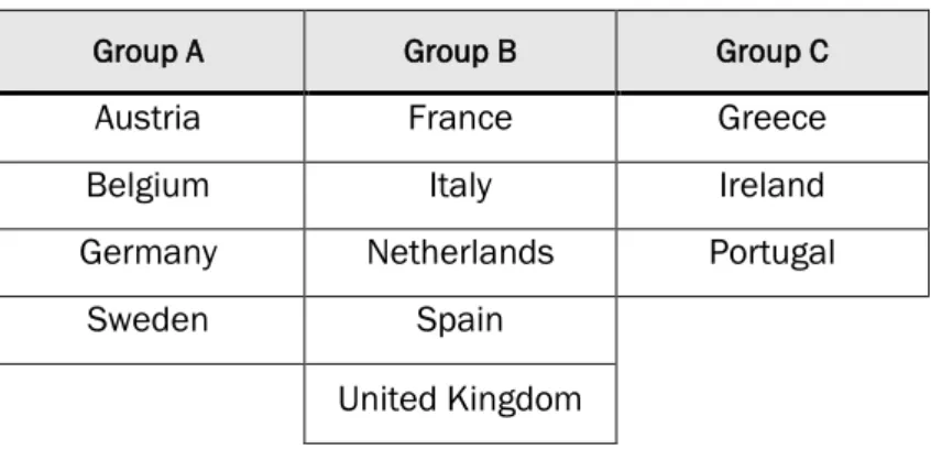
Table 1. Groups and Countries used in Data Set.
Group A Group B Group C
Austria France Greece
Belgium Italy Ireland
Germany Netherlands Portugal
Sweden Spain
United Kingdom
Group A
The first group is composed by countries that seem to be directly less affected by the crisis: Austria, Belgium, Germany and Sweden.
These countries have in common the positive average growth rates obtained in the Post Crisis period, which were comprised between 0.395 p.p. (Austria) and 1.126 p.p. (Sweden), as noticeable in Table C 1
.
Despite the clear fall down of the average GDP growth rate from Pre to Post Crisis, these countries had a common growth rate path along the Post Crisis (Figure C 2).The lowest average Post-Crisis Deficit ratios were also displayed in this group (between -3.933 p.p. in Belgium and -0.800 p.p. in Sweden), and the growth of Deficit ratios from Pre to Post Crisis Period was not as accentuated as in the other countries of the sample. Regarding the evolution of Gross Debt, there are clear differences among countries, since Belgium had already in Pre Crisis a significant average Gross Debt of 100.60 p.p. of the country´s GDP, in contrast to Sweden, where the Gross Debt was below the 50 p.p. However, the increase of the Post Crisis Average Gross Debt in Belgium was marginal (about of 2 p.p), while in Austria and Germany it increased about 15 p.p., and Sweden it decreased about 9 p.p.
13
Group B
The second sub-group of countries is composed by France, Italy, Netherlands, Spain and United Kingdom. These countries displayed high average GDP growth rates (above 1 p.p.) in the Pre-Crisis period and a clear deceleration of the economy during the Post-Crisis period, with negative average GDP growth rates in Italy, Netherlands and Spain and positive average rates below 1 p.p. in France and United Kingdom, as shown in Table C 1.
Moreover, all countries of Group B presented an increase above 14 p.p of the average Gross Debt, from Pre to Post-Crisis Period, and a similar scenario is presented in terms of Deficit ratios – all countries presented a deficit higher than 3 p.p. in the Post-Crisis period.
In Figure C 3 is noticeable the discrepancies in terms of real growth rate among countries, which highlights this group as less homogeneous than group A.
Group C
The last group is composed by the countries that were directly more affected by the crisis: Greece, Ireland and Portugal. These countries faced the intervention and the assistance of the European Commission (EC), the European Central Bank (ECB) and the International Monetary Fund (IMF), due to unsustainable government debt over 100 p.p of the GDP.
In terms of Real GDP Growth Rate during the Post-Crisis period, both Greece and Portugal possessed the lowest average rates in the sample EU countries (-4.793 p.p. and -1.193 p.p.), with a similar path from 2012 to 2014, as noticed in Figure C 4, while Ireland severely decelerated its economy but remained with positive growth rates during the Post Crisis Period.
Furthermore, these three countries presented high deficit ratios with a clear worsening scenario during the Post Crisis Period, particularly in Greece and Ireland with average Deficit above 10 p.p of GDP, but also in Portugal, where it surpassed 7 p.p.
14
4.3 Input and Output Variables
The nature of banking technology and the definition and measurement of inputs, outputs and factor prices to be applied for bank efficiency analysis have been widely discussed by a vast literature in the last decades. The discussion derived from the treatment of “deposits” as an input or an output in the production function and it resulted in two different approaches: 1) the intermediation approach, exposed by Sealey and Lindley (1977) , which considers banks as intermediaries between the supply and the demand, transforming deposits and liabilities from savers into loans and other assets to investors, thus, it considers deposits as an input; and 2) the production approach (Sherman and Gold, 1985), which views banks as firms that use capital and labor as inputs to provide financial services such as loans and deposits, which came to be an output in the production function
This work follows the intermediation approach, as it is considered more appropriate to evaluate the efficiency of financial institutions due to the fact that it includes interest expenses in the functional function, which represent a large portion of total costs (Berger and Humphrey 1997). Moreover, Hughes and Mester (1993) indicated that insured and uninsured deposits are inputs in all bank size categories in a test to determine how to treat deposits in the production function.
For this analysis it will be only considered the annual consolidated financial statements of the agglomerate data of commercial and savings banks collected from Bankscope International Database. This data was chosen to guarantee the homogeneity of the sample and to minimize the risk of disparities in efficiency scores due to different production technologies and/or banking structure along institutions (Bos and Schmiedel 2007; Fitzpatrick and McQuinn 2005). All data is reported in Euro as the reference currency.
The implementation of the DEA model was based in three outputs (Y1=Total Loans, Y2=
Other Earning Assets; Y3 = Other Operating Income) and three inputs (X1= Deposits and Short
Term Funding, X2 = Other Interest Bearing Liabilities and X3= Loan Loss Provisions), following
15
The first output variable considered on the functional form is Total Loans which captures the traditional lending activity of banks and it is composed by Gross Loans and Reserves for Impaired Loans (Alzubaidi and Bougheas 2012). The data of this variable is exposed in Table D 2.
The second output variable is Other Earning Assets, which represents the non-lending activity of banks and is comprised of Loans and Advances to Banks, Derivatives, Other Securities and Remaining Earning Assets (see Table D 3).
Other Operating Income is also included as an output because modern banking institutions have been following a diversification strategy and thus, off-balance sheet components increased its relevance on banks accounts (Drake and Hall, 2003 and Drake et. al., 2009). The data of this variable is exposed in Table D 4.
The first input chosen is Deposits and Short Term Funding which is composed by three different components: Total Customer Deposits, Deposits from Banks and Other Deposits and Short Term Borrowings. The inclusion of this input is crucial since it englobes the non-traditional business activities undertaken by the bank (Alzubaidi and Bougheas 2012). The data of this variable is exposed in Table D 5.
Another input specified is the variable Other Interest Bearing Liabilities which includes Derivatives, Trading Liabilities and Long Term Funding components trading from banks. On this input it was necessary to use a proxy for Greece data between 2000 and 2003 since DEA program does not recognize zero as a valid value. Therefore, it was assumed for those years a growth rate of 9%, the average growth rate of this input from 2004 until 2014 (see Table D 6).
The third input is Loan Loss Provisions, presented in the income statement, which represents the expenses set aside for uncollected loan payments, i.e., it is used as proxy for the risk of lending default (Alzubaidi and Bougheas 2012). Again a proxy was used for negative results. It was assumed a marginal result for the lowest value (above 1 million euros
16
in Germany in 2011), and a proportional result for the remaining negative values over the sample data (see Table D 7).
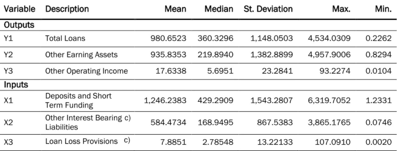
The disparities in the sample EU economies are also perceptible analyzing the input and output bank levels (Table 2) since variables such as Total Loans, Other Earning Assets and Deposits and Short Term Funding show a standard deviation superior to 1,000 million euros and, in general. there is a considerable gap between minimum and maximum values for each variable, sustaining the view of an unbalanced EU in terms of size, growth and other macroeconomic indicators.
Table 2. Descriptive Statistics of Bank Level Variables
Source: Authors´ calculations using the agglomerate consolidated data from BankScope Database. a) All values expressed in millions of Euro.
b) Approximation values with four decimal numbers. c) All values assuming the used proxies for variables.
Variable Description Mean Median St. Deviation Max. Min. Outputs
Y1 Total Loans 980.6523 360.3296 1,148.0503 4,534.0309 0.2262
Y2 Other Earning Assets 935.8353 219.8940 1,382.8899 4,957.9006 0.8294
Y3 Other Operating Income 17.6338 5.6951 23.2841 93.2274 0.0104
Inputs
X1 Deposits and Short Term Funding 1,246.2383 429.2909 1,543.2807 6,319.7052 1.2331 X2 Other Interest Bearing Liabilities 584.4734 168.9495 867.5383 3,865.1765 0.0746
X3 Loan Loss Provisions 7.8851 2.78548 13.22133 107.0910 0.0020
c) c)
17 0,00 0,20 0,40 0,60 0,80 1,00 2000 2001 2002 2003 2004 2005 2006 2007 2008 2009 2010 2011 2012 2013 2014
Technical Efficiency Allocative Efficiency Cost Efficiency
5. Empirical Results
The Data defined before was used to run DEA results, creating a common efficient frontier for all DMU´s in each year, which allow a comparison of efficient scores across sample countries against a common benchmark.
This section initially examines the general evolution of the allocative, technical and cost efficiency levels along the time period stipulated for this study, for posterior detailed comparison in terms of Groups defined in Data, from Pre to Post-Crisis periods.
5.1 EU Banking Efficiency Evolution
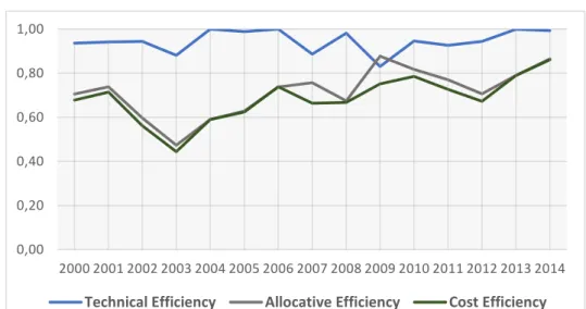
The evolution of Technical, Allocative and Cost Efficiency Levels is exposed in Figure 1, from which some conclusions can be taken: overall, commercial and savings banks of the sample of all considered EU countries presented higher technical efficiency than allocative and cost efficiency levels. The overall mean of cost efficiency over the sample period was about 68.5 p.p., indicating that banks could make costs savings up to 31.5 p.p., while the mean of allocative and technical efficiency levels were about 71.5 and 94.7, respectively. These findings suggest that the allocative component contributed significantly to cost inefficiency, as perceptible on Figure 1, since patterns of allocative and cost efficiency levels are very similar, particularly in the Pre-Crisis Period and the last three years of the sample.
Figure 1. Evolution of Efficiency Levels over Time.
18
In years of 2002 and 2003, the overall economic efficiency reached the lowest values of all sample period with 52 p.p. and 44 p.p. respectively. However, after this period and until the financial crisis it was shown a remarkable and general improvement of efficiency, being particularly noticeable in all efficiency levels in year of 2004.
The boost of financial crisis in 2007 delivered severe oscillations on efficiency levels: for instance, the allocative efficiency was not affected and raised about 2 p.p. while technical efficiency lowered about 10 p.p., leading to a fall of cost efficiency of about 8 p.p.
On the following year the positions were inverted with a reduction of the allocative efficiency and an increase of technical efficiency, both of 9 p.p. Finally, in 2009, these two efficiency levels achieved a maximum and a minimum level, surpassing the 80 p.p. efficiency level. Furthermore, the average allocative efficiency level was higher than the average technical efficiency level, an exception over the period of time analyzed. Hence it can be said that, in the particular year of 2009, the EU banks, on average, were closer to use inputs in optimal proportions regarding the respective prices, than to maximize the output given a set of inputs. In prima facie, this seems to be an answer of the EU banks to the crisis installed in the year before, a specific situation that was reversed in the following years since the overall allocative efficiency decreased vertiginously until 2012 while the overall technical efficiency raised to levels near to the maximum efficiency.
In 2012, a similar situation as in 2003 was observable, with a substantial increase of all efficiency levels in the last two years of the sample. In the last year, 2014, the overall cost efficiency reached the highest efficiency level of the whole sample (86 p.p.), as result of the reduction of the overall allocative inefficiency (below 20 p.p.) and the maintenance of elevated levels of technical efficiency across sample countries.
19
5.2 Cost Efficiency Results
In this chapter is reported average cost efficiency levels of the whole sample countries for the subsequent division by Groups stipulated in Data.
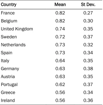
Table 3 summarizes the average cost efficiency levels of banks of the selected EU countries, by descendent numerical order. The Sample Statistics show that the average efficiency scores on the selected countries were comprised between 56 and 82 p.p., and there were significant efficiency fluctuations over years since the standard deviation of DEA results are relatively high (over 0.27 in all countries).
Table 3. Descriptive Statistics of Cost Efficiency Results
Source: Author´s calculations using Data from DEA 2.1 software program.
On average the banks with the highest cost efficiency levels were located in France, Belgium and United Kingdom, with average results between 74 and 82 p.p.
On the opposite side the countries with the lowest average levels were precisely the countries that required economical and financial intervention: Greece and Ireland both with 56 p.p., followed by Portugal with 62 p.p. These results were, in some extent, influenced by the low efficiency levels during the crisis in 2007 and 2008, particularly in Greece and
Country Mean St Dev.
France 0.82 0.27 Belgium 0.82 0.30 United Kingdom 0.74 0.35 Sweden 0.72 0.37 Netherlands 0.73 0.32 Spain 0.73 0.34 Italy 0.64 0.35 Germany 0.63 0.38 Austria 0.63 0.35 Portugal 0.62 0.37 Greece 0.56 0.34 Ireland 0.56 0.36
20
Ireland, where the maximum attained was below 50 p.p., and even afterwards the scores remained substantially low (Table 4). For instance, in the last year (2014), the scores obtained were about 36 and 33 p.p. respectively, far below the average of the sample which was about 86 p.p. In the case of Portugal, the efficiency results derived from the bank performance during the Pre-Crisis Period.
It is also relevant to analyze the cost efficiency results of Germany, the largest economy in Europe. The poor results obtained (an average of 63 out of 100 p.p.) contrast to the solid macroeconomic indicators shown in the last 15 years with GDP growth rates above 1 p.p. and low Gross Debt and Deficit ratios in comparison to other EU economies. Moreover, as shown by the high standard deviation, the DEA results were extremely volatile with severe oscillations along years, taking emphasis the lowest result in 2007 of only 9 p.p., far below the sample average of about 66 p.p. In fact, in about half of the sample period, the DEA results of the country were below the average of the sample countries results which highlighted the poor performance of German banks following the DEA method. This result is in line with Casu and Girardone (2010) which classified Germany as one of the less efficient in EU-15 with a similar average of 60 p.p. in the period 2000-2005.
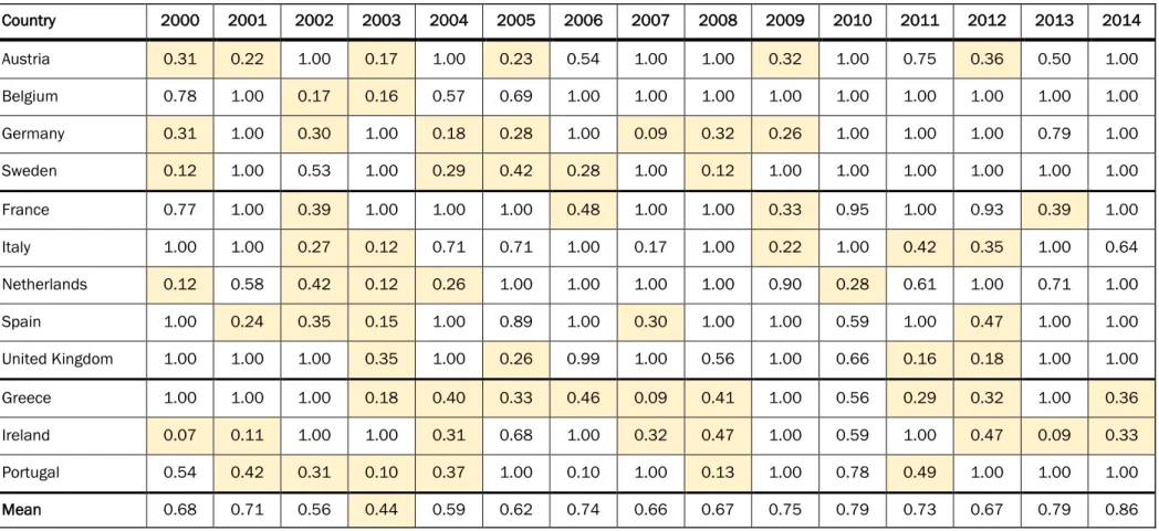
Beyond this, all countries presented low DEA levels (below 20 p.p.) in a specified year. It takes emphasis the year of 2003, where about half of the countries sample obtained the lowest level, which justifies the low average cost efficiency obtained in that year. In contrast, in the last year of the sample 9 out of 12 countries reached the maximum efficiency level (exception of Greece, Ireland and Italy) which consists the year with the highest number of DMUs reaching 100 p.p. over the sample period.
21
Source: DEA Results obtained from DEA 2.1 software program.
Country 2000 2001 2002 2003 2004 2005 2006 2007 2008 2009 2010 2011 2012 2013 2014 Austria 0.31 0.22 1.00 0.17 1.00 0.23 0.54 1.00 1.00 0.32 1.00 0.75 0.36 0.50 1.00 Belgium 0.78 1.00 0.17 0.16 0.57 0.69 1.00 1.00 1.00 1.00 1.00 1.00 1.00 1.00 1.00 Germany 0.31 1.00 0.30 1.00 0.18 0.28 1.00 0.09 0.32 0.26 1.00 1.00 1.00 0.79 1.00 Sweden 0.12 1.00 0.53 1.00 0.29 0.42 0.28 1.00 0.12 1.00 1.00 1.00 1.00 1.00 1.00 France 0.77 1.00 0.39 1.00 1.00 1.00 0.48 1.00 1.00 0.33 0.95 1.00 0.93 0.39 1.00 Italy 1.00 1.00 0.27 0.12 0.71 0.71 1.00 0.17 1.00 0.22 1.00 0.42 0.35 1.00 0.64 Netherlands 0.12 0.58 0.42 0.12 0.26 1.00 1.00 1.00 1.00 0.90 0.28 0.61 1.00 0.71 1.00 Spain 1.00 0.24 0.35 0.15 1.00 0.89 1.00 0.30 1.00 1.00 0.59 1.00 0.47 1.00 1.00 United Kingdom 1.00 1.00 1.00 0.35 1.00 0.26 0.99 1.00 0.56 1.00 0.66 0.16 0.18 1.00 1.00 Greece 1.00 1.00 1.00 0.18 0.40 0.33 0.46 0.09 0.41 1.00 0.56 0.29 0.32 1.00 0.36 Ireland 0.07 0.11 1.00 1.00 0.31 0.68 1.00 0.32 0.47 1.00 0.59 1.00 0.47 0.09 0.33 Portugal 0.54 0.42 0.31 0.10 0.37 1.00 0.10 1.00 0.13 1.00 0.78 0.49 1.00 1.00 1.00 Mean 0.68 0.71 0.56 0.44 0.59 0.62 0.74 0.66 0.67 0.75 0.79 0.73 0.67 0.79 0.86
Table 4. Cost Efficiency Results
22
Despite the relevance of results obtained, the above-mentioned analysis does not allow to conclude the evolution of efficiency levels across countries. Therefore, it is relevant an extension of this study, namely, a cross country comparison by period of time in order to analyze the main effects of the financial crisis on the bank performance of the considered countries.
There were noticeable severe fluctuations in all countries along the three periods of time. Particularly during the first period of time, the standard deviation was high and show the oscillations presented on bank efficiency from one year to the following one. This scenario had changed during the crisis period, since some countries (Austria, Belgium, France and Netherlands) were fully efficient and therefore had a null standard deviation, while others, such as Sweden, Italy, Spain and Portugal, maintained extremely volatile efficiency levels, and the countries most affected during financial crisis in terms of banking efficiency (Germany, Greece and Ireland) exhibited lower standard deviation levels.
Group A
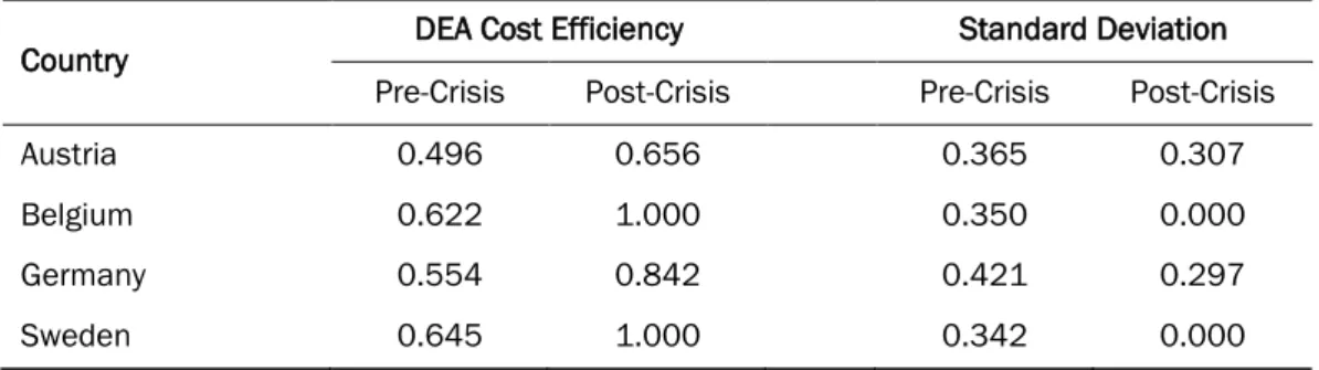
All countries of Group A presented an increase on average DEA levels from Pre to Post-Crisis Period and a subsequent reduction of standard deviation, which induces an improvement of banking efficiency and its stability along time period (Table 5).
The year-to-year efficiency disparities in Pre-Crisis contrasts to a Post-Crisis Period where all countries possess yearly efficiency levels near or equal to 100 p.p. (with the exception of Austria in 2012 and 2013), being noticeable the increase of cost efficiency of about 35 p.p. in banks from Belgium and Sweden, which attained the maximum efficiency level during the whole Post-Crisis Period. These results are particularly relevant since both countries had shown during the Pre-Crisis a high volatility level of DEA results in yearly basis, while during the Crisis Period, Belgium was fully efficient and Sweden reached the lowest level of efficiency in 2009, meaning that countries’ path present some differences.
23 Table 5. Comparison of Cost Efficiency – Group A
Country DEA Cost Efficiency Standard Deviation Pre-Crisis Post-Crisis Pre-Crisis Post-Crisis
Austria 0.496 0.656 0.365 0.307
Belgium 0.622 1.000 0.350 0.000
Germany 0.554 0.842 0.421 0.297
Sweden 0.645 1.000 0.342 0.000
Source: Author ´s calculations from DEA 2.1. software program
Group B
Group B displays the largest variety of results, explained in part by the different effects of financial crisis in the respective economies.
A wide efficiency gap of about 24 p.p. is shown among countries during the Post-Crisis, explained by a reduction of efficiency levels in France, Italy and UK and an increase in Netherlands and Spain (Table 6). These discrepancies are also corroborated in terms of the standard deviation of the cost efficiency results since it was observable an increase of efficiency´s dispersion in banks from France, Italy and UK, the most affected in terms of efficiency, which turned to show high volatility along the years, while in the remaining countries, the results became more concentrated.
Table 6. Comparison of Cost Efficiency – Group B
Country DEA Cost Efficiency Standard Deviation Pre-Crisis Post-Crisis Pre-Crisis Post-Crisis
France 0.839 0.768 0.276 0.317
Italy 0.685 0.604 0.364 0.336
Netherlands 0.625 0.751 0.377 0.277
Spain 0.662 0.843 0.394 0.246
United Kingdom 0.799 0.668 0.340 0.406 Source: Author ´s calculations from DEA 2.1. software program
24
Group C
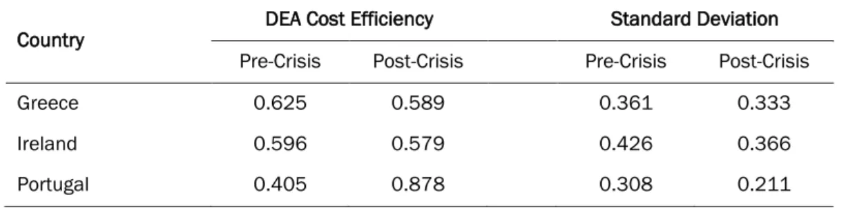
In Group C, Greece and Ireland presented the lowest cost efficiency scores for the last five years of the sample with about 58.9 and 57.9 p.p., respectively. On the opposite side, Portugal had shown a positive evolution along the three periods, being the only country in this situation and the one with the highest increase (of about 47 p.p.) of DEA levels when comparing Pre and Post Crisis Period. It is also remarkable the reduction of standard deviation in all countries, which follows the overall scenario and demonstrate a significant reduction of year-on-year efficiency oscillations (Table 7).
Table 7. Comparison of Cost Efficiency – Group C
Country DEA Cost Efficiency Standard Deviation Pre-Crisis Post-Crisis Pre-Crisis Post-Crisis
Greece 0.625 0.589 0.361 0.333
Ireland 0.596 0.579 0.426 0.366
Portugal 0.405 0.878 0.308 0.211
Source: Author ´s calculations from DEA 2.1. software program
An overall analysis of the obtained results demonstrates the maintenance of a significant efficiency´s gap among countries in the Post-Crisis. Nonetheless, both lower and upper efficiency levels increased from Pre to Post-Crisis, with a significant positive variation over 16 p.p. in both cases (Table E 1).
This analysis reveals that the financial crisis did not contribute to an EU Multi Speed Banking Efficiency because during the Pre-Crisis the discrepancies were already accentuated. However, as referred, the year on year fluctuations of DEA results does not allow a strict and concise subdivision of countries in terms of banking efficiency.
25
5.3 Technical and Allocative Efficiency Results
This sub-section offers an analysis of the evolution of the two components of overall economic efficiency: technical efficiency (TE), which reflects the ability of banks to maximize bank outputs from defined inputs, and allocative efficiency (AE), which induces how efficient a firm uses the inputs in the production process, given their respective prices.
Table 8 exhibits the descriptive statistics of technical and allocative efficiency results obtained from DEA program. Table 9 and Table 10 present the technical and allocative efficiency scores for each sample country over the period 2000-2014.
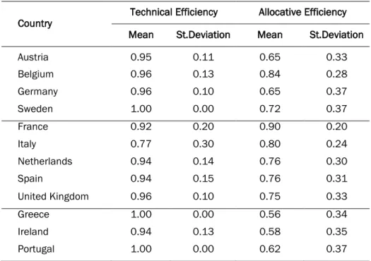
The results obtained allow to conclude that, in general, the countries present higher average levels of technical than allocative efficiency. There is also a reduced dispersion of technical efficiency levels along time since the standard deviation of DEA results are particularly low.
Hence, the countries’ average cost efficiency is very close to the respective average allocative efficiency, being even similar in the case of three countries (Sweden, Greece and Portugal) since they were fully technical efficient along time.
Table 8. Technical and Allocative Efficiency
Country Technical Efficiency Allocative Efficiency Mean St.Deviation Mean St.Deviation
Austria 0.95 0.11 0.65 0.33 Belgium 0.96 0.13 0.84 0.28 Germany 0.96 0.10 0.65 0.37 Sweden 1.00 0.00 0.72 0.37 France 0.92 0.20 0.90 0.20 Italy 0.77 0.30 0.80 0.24 Netherlands 0.94 0.14 0.76 0.30 Spain 0.94 0.15 0.76 0.31 United Kingdom 0.96 0.10 0.75 0.33 Greece 1.00 0.00 0.56 0.34 Ireland 0.94 0.13 0.58 0.35 Portugal 1.00 0.00 0.62 0.37 Source: Author ´s calculations from DEA 2.1. software program
26
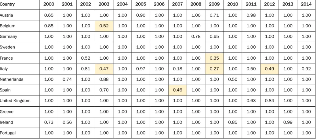
Table 9. Technical Efficiency Results
Country 2000 2001 2002 2003 2004 2005 2006 2007 2008 2009 2010 2011 2012 2013 2014 Austria 0.65 1.00 1.00 1.00 1.00 0.90 1.00 1.00 1.00 0.71 1.00 0.98 1.00 1.00 1.00 Belgium 0.85 1.00 1.00 0.52 1.00 1.00 1.00 1.00 1.00 1.00 1.00 1.00 1.00 1.00 1.00 Germany 1.00 1.00 1.00 1.00 1.00 1.00 1.00 1.00 0.78 0.65 1.00 1.00 1.00 1.00 1.00 Sweden 1.00 1.00 1.00 1.00 1.00 1.00 1.00 1.00 1.00 1.00 1.00 1.00 1.00 1.00 1.00 France 1.00 1.00 0.52 1.00 1.00 1.00 1.00 1.00 1.00 0.35 1.00 1.00 1.00 1.00 1.00 Italy 1.00 1.00 0.81 0.47 1.00 0.97 1.00 0.18 1.00 0.27 1.00 0.50 0.49 1.00 0.92 Netherlands 1.00 0.74 1.00 0.88 1.00 1.00 1.00 1.00 1.00 1.00 0.50 1.00 1.00 1.00 1.00 Spain 1.00 1.00 1.00 0.70 1.00 1.00 1.00 0.46 1.00 1.00 1.00 1.00 1.00 1.00 1.00 United Kingdom 1.00 1.00 1.00 1.00 1.00 1.00 1.00 1.00 1.00 1.00 1.00 0.63 0.84 1.00 1.00 Greece 1.00 1.00 1.00 1.00 1.00 1.00 1.00 1.00 1.00 1.00 1.00 1.00 1.00 1.00 1.00 Ireland 0.73 0.56 1.00 1.00 1.00 1.00 1.00 1.00 1.00 1.00 0.85 1.00 1.00 0.99 1.00 Portugal 1.00 1.00 1.00 1.00 1.00 1.00 1.00 1.00 1.00 1.00 1.00 1.00 1.00 1.00 1.00
Source: Data obtained from calculations using DEA 2.1. Software Notes: The TE levels below 50 p.p. are shaded in yellow.
27
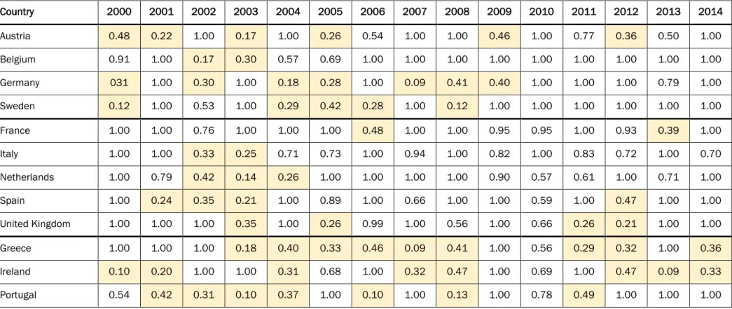
Table 10. Allocative Efficiency Results
Country 2000 2001 2002 2003 2004 2005 2006 2007 2008 2009 2010 2011 2012 2013 2014 Austria 0.48 0.22 1.00 0.17 1.00 0.26 0.54 1.00 1.00 0.46 1.00 0.77 0.36 0.50 1.00 Belgium 0.91 1.00 0.17 0.30 0.57 0.69 1.00 1.00 1.00 1.00 1.00 1.00 1.00 1.00 1.00 Germany 031 1.00 0.30 1.00 0.18 0.28 1.00 0.09 0.41 0.40 1.00 1.00 1.00 0.79 1.00 Sweden 0.12 1.00 0.53 1.00 0.29 0.42 0.28 1.00 0.12 1.00 1.00 1.00 1.00 1.00 1.00 France 1.00 1.00 0.76 1.00 1.00 1.00 0.48 1.00 1.00 0.95 0.95 1.00 0.93 0.39 1.00 Italy 1.00 1.00 0.33 0.25 0.71 0.73 1.00 0.94 1.00 0.82 1.00 0.83 0.72 1.00 0.70 Netherlands 1.00 0.79 0.42 0.14 0.26 1.00 1.00 1.00 1.00 0.90 0.57 0.61 1.00 0.71 1.00 Spain 1.00 0.24 0.35 0.21 1.00 0.89 1.00 0.66 1.00 1.00 0.59 1.00 0.47 1.00 1.00 United Kingdom 1.00 1.00 1.00 0.35 1.00 0.26 0.99 1.00 0.56 1.00 0.66 0.26 0.21 1.00 1.00 Greece 1.00 1.00 1.00 0.18 0.40 0.33 0.46 0.09 0.41 1.00 0.56 0.29 0.32 1.00 0.36 Ireland 0.10 0.20 1.00 1.00 0.31 0.68 1.00 0.32 0.47 1.00 0.69 1.00 0.47 0.09 0.33 Portugal 0.54 0.42 0.31 0.10 0.37 1.00 0.10 1.00 0.13 1.00 0.78 0.49 1.00 1.00 1.00
Source: Data obtained from calculations using DEA 2.1. Software Notes: The AE levels below 50 p.p. are shaded in yellow.
28
Banks from Italy are figured as the exception, since the average allocative efficiency score is higher than the average technical efficiency score, which is far below the remaining countries and the overall average.
As conclusion, European banks were, in general, able to fully maximize the output using a given set of inputs. However, the inputs applied by banks were not being used in optimal proportions, i.e., European banks were in some extent “allocative inefficient” since it was possible to produce the same amount of output taken a lower input cost.
Group A
Table 11 exhibits the main changes of both technical and allocative efficiency levels from Pre to Post Crisis periods. The improvement of efficiency scores is substantially higher in terms of allocative efficiency than in technical efficiency, which is in line with the overall results of the sample. This does not seem a surprise since banks from these countries were almost technical efficient in Pre Crisis with average levels above 90 p.p., while they still possessed allocative inefficiencies over 40 p.p.
However, there are clear disparities among countries. While, Belgium and Sweden displayed the maximum efficiency level in both efficiency types during the post crisis period, with reductions of allocative inefficiency of 33 p.p. and 48 p.p., respectively, Austria reduced its allocative inefficiency in only 16 p.p., and exhibited an average level far below the remaining countries of the group A, and Germany was the only country in which a slight decrease of technical efficiency can be observed, which turned to be compensated by an increase over 28 p.p. in terms of allocative efficiency. This is an interesting result since it is in line with the efficiency levels observed in 2009, where there was a major concern of allocative in harm of technical efficiency.
29
Table 11. Comparison of Technical and Allocative Efficiency – Group A
Source: Author ´s calculations from DEA 2.1. software program
Group B
As well as in case of macroeconomic indicators, the countries belonging to group B present a large heterogeneity level, without a particular trend or path along time. In terms of both technical and allocative efficiency levels, it takes emphasis the movements of efficiency results of banks located in Italy. In the Pre-Crisis, both efficiency levels were above 70 p.p., while in the Post-Crisis, allocative levels increased over 13 p.p. and technical levels fell down about 20 p.p. (Table 12). Thus, Italian commercial and savings banks became aware of the relevance of allocative efficiency but they were not capable of maintaining the elevated TE levels over time, resulting in the fall of cost efficiency levels already presented.
Table 12. Comparison of Technical and Allocative Efficiency – Group B
Source: Author ´s calculations from DEA 2.1. software program
Technical Efficiency Allocative Efficiency Pre Crisis Post Crisis Pre Crisis Post Crisis Austria 0.935 0.948 0.524 0.680 Belgium 0.909 1.000 0.664 1.000 Germany 1.000 0.941 0.581 0.865
Sweden 1.000 1.000 0.520 1.000
Technical Efficiency Allocative Efficiency Pre Crisis Post Crisis Pre Crisis Post Crisis
France 0.931 0.891 0.891 0.871
Italy 0.893 0.696 0.715 0.843
Netherlands 0.946 0.916 0.658 0.799
Spain 0.957 1.000 0.671 0.843
30
In a different scenario were banks from Netherlands and Spain that increased substantially the respectively allocative efficiency levels without threatening the technical efficiency levels, since Netherlands reduced their average level marginally (3 p.p.) and Spain reached the maximum level in the Post Crisis Period.
Finally, both France and UK presented some similarities in terms of evolution of efficiency levels since a reduction of efficiency is visible in both countries, being particularly accentuated in UK.
Group C
The countries that required economical and financial intervention bring also relevant and interesting results, since both banks from Greece and Portugal possessed the maximum technical efficiency levels in both periods, meaning that countries, in response to the financial crisis of 2007-08, were capable to maximize outputs obtained from the respective inputs variables, and banks headquartered in Ireland increased about 8 p.p. the average technical efficiency levels (Table 13).
However, in terms of allocative efficiency the results are dissonant: banks located in Greece and Ireland observed inefficiency levels over 40 p.p., while the inefficiency level in Portuguese banks was below 12 p.p. The huge discrepancy of allocative efficiency levels from Pre to Post Crisis (a gap over 40 p.p.) may derive from different reasons, namely banking restructuring and bailout processes as well as M&A processes.
Table 13. Comparison of Technical and Allocative Efficiency – Group C
Source: Author ´s calculations from DEA 2.1. software program
Technical Efficiency Allocative Efficiency Pre Crisis Post Crisis Pre Crisis Post Crisis Greece 1.000 1.000 0.625 0.589 Ireland 0.899 0.974 0.613 0.596 Portugal 1.000 1.000 0.405 0.878
31
Examining the overall technical efficiency results, reported in Table E 1, it is perceptible an increase of the efficiency´s gap among countries from 10.7 p.p. in Pre-Crisis to 30.4 p.p. in Post-Crisis, as result of the worsening performance of Italian banks, that suffered a reduction of 19.7 p.p. from Pre to Post-Crisis.
In terms of allocative efficiency results, there was a marginal reduction of efficiency´s gap from Pre to Post-Crisis of 7.5 p.p., due to an increase of both lower and upper levels. This reflects the awareness of sample EU banks to optimize factor inputs in terms of the respective prices, a feature that was neglected in some countries in the initial sample years.
The above-mentioned results follow, in some extent, the path of cost efficiency results exposed before, which reinforces the idea that allocative inefficiency contributed to cost inefficiency. This results from the elevated technical efficiency results since the cost efficiency level corresponds to the product of the allocative and the technical efficiency levels (see Figure A 1).
Over the sample defined, about 83.89 p.p. of the cases the banks were considered fully technical efficient (TE level equal to 100 p.p.). The data calculated also show that banks from sample countries were only allocative and cost efficient in about 47.78 p.p. of the cases, and that the quartile frequencies of both levels are particularly similar.
32
6. Conclusions and Final Remarks
This paper aimed to provide empirical evidence of a relationship between macroeconomic environment and bank cost efficiency in European Union, trying to answer the question of a multi-speed EU banking efficiency along the years and the effect of the financial crisis of 2007-08 on the efficiency levels across EU countries.
Following that propose, this study analyzed the evolution of the technical, allocative and cost efficiency results in 12 EU countries from 2000 to 2014. The dataset was represented by a panel that covers the annual agglomerate and consolidated financial statement accounts of the commercial and savings banks headquartered in Austria, Belgium, France, Germany, Greece, Ireland, Italy, Netherlands, Portugal, Spain, Sweden and United Kingdom, using data extracted from BankScope International Database. The countries were subdivided in three groups, according to the macroeconomic situation analyzed over the Data of Real GDP Growth Rate, Deficit and Government Debt Ratios, extracted from World Bank and Eurostat Databases.
The Methodology used to measure Bank Cost Efficiency was the Data Envelopment Analysis (DEA), a non-parametric approach, that yields a convex frontier set composed by the best practices among the sample observations. Following the intermediation approach, three Inputs (Deposits and Short Term Funding; Other Interest Bearing Liabilities and Loan Loss Provisions) and three Outputs (Total Loans; Other Earning Assets and Other Operating Income) were defined as the Bank Level Variables used in the model function.
The main findings point out an overall improvement of cost efficiency, with a reduction of the overall inefficiency levels over 18 p.p. and a reduction of the standard deviation among observations of about 16 p.p. from 2000 to 2014.
Nevertheless, the financial crisis affected the commercial and savings banks headquartered in the sample countries since a significant fall of the overall cost efficiency was displayed in 2007 and continuous yearly efficiency´s oscillations were observed among countries. This is in line with the findings of Alzubaidi and Bougheas (2012), who mention the