Does the private database help to explain Brazilian inflation?
Emerson Fernandes Mar¸cala
, Pedro Vallsb
, and Diogo de Princec
aSao Paulo School of Economics and CEMAP, FGV. Rua Itapeva 286, 10o andar ZIP code: 01332-000 Sao Paulo, SP, Brazil
bSao Paulo School of Economics and CEMAP, FGV. Rua Itapeva 474, 10o andar ZIP code: 01332-000 Sao Paulo, SP, Brazil,
E-mail: Corresponding author - [email protected] cUNIFESP
January 2019
Abstract
The large dimension of variables as regressors requires a reduction in the number of variables, which we do in this paper through the factorial model. This method is useful if the variables are collinear, as is our case. We aim to synthesize information from Brazilian Institute of Economics (IBRE)’s public and private databases to evaluate if there is an additional gain from the private database to explain the Brazilian inflation index, the broad consumer price index (IPCA). We analyze the monthly period between 2000 and 2018. After we extract factor, we select which factors are relevant regressors to explain inflation with the Autometrics algorithm. Our result is that the factors extracted from the public database bring gains to explain inflation in relation to an autoregressive model. However, the use of factors tied to the private database still leads to explanatory gains for inflation. We have been able to explain about 75% of the inflation variations with the use of the factors extracted from the private and public databases.
1 Introduction
When we have a large dimension of variables as regressors, one point to address is the reduction of dimensionality. In general, there is no particular reason to choose a particular measure of the variable. For example, in the case of interest rates, we can use the basic interest rate of the economy, the interest rate paid by government bonds, forward rates, among others. Another point that is unclear is whether it is more appropriate to use the aggregate variable or its disaggregated measures to explain inflation (using industrial production or decomposing into sectors). If we choose among variables, it introduces an element of arbitrariness and it can lead to misspecification and misleading results (Hansen and Richard (1987), Ludvigson and Ng (2007)). In this case, we can consider one method to summarize the information of the different (and different measures of) variables for example.
When the potential variable dimension is greater than the sample size, we can not use some variable selection methods. In addition, methods such as least absolute shrinkage and selection operator (Lasso) work best in cases where variables are not highly correlated, which is not the case for most applications in economics. The factor methods are particularly useful for dimensionality reduction when the variables are collinear (Elliott and Timmermann (2016)). This is the intuition for us to use the factor method to achieve dimensionality reduction in this research and it can summarize the information in large data sets with minimal loss of information. If we use the joint information (comovement) between the variables of the database through a small number of factors, this approach is more parsimonious and it provides protection against data irregularities (Bernanke et al. (2005)).
We aim to synthesize information from Brazilian Institute of Economics (IBRE)’s public and private databases to evaluate if there is an additional gain from the private database to explain the Brazilian inflation index, the broad consumer price index (IPCA). We analyze the monthly period between 2000 and 2018. We extract the factors from three different databases: (i) only public data, (ii) only private data, and (iii) the combination of public and private data. We decide the number of factors to be extracted from each database based on Bai and Ng (2002)). We select which factors are relevant regressors to explain inflation with the Autometrics algorithm considering the possibility of the presence of dummy variables (to control the presence of structural breaks or outliers) and allowing the autoregressive component of inflation.
Our article has five sections besides this introduction. The second section synthesizes the litera - ture on extracting factors to monitor, explain or predict inflation. We present the methodology in the third section, followed by the data used and the strategy we adopt in the fourth section. The fifth section presents the results and finally we discuss the final considerations of the article.
2 Literature Review
Variable selection methods choose a small subset of predictors from a large set of potentially useful variables. Instead of selecting a few predictors, Stock and Watson (2002, 2011, 2016) and Ban´bura et al. (2013), among others, deal with the approach to summarize the information of all candidate predictors by a number of factors especially in macroeconomics.
The factors extracted from macroeconomic data capture the comovement between the series. For example, consider extracting one factor from three highly correlated series such as Gross Domestic Product (GDP), employment, and industrial production. This factor is related to the comovement of the output of the economy for example. If we use the joint information (comovement) between these three variables through one factor, this approach is more parsimonious and it provides protection against data irregularities (Bernanke et al. (2005)).
As the factors capture the comovements, an application for the factors is to allow the macroeco- nomic monitoring. That is, we can construct an index of economic activity indicators from factors extracted from economic activity data. For example, the first factor is a natural index of move- ments of the relevant time series of economic activity. Stock and Watson (1989, 1991) create an experimental coincident index (XCI) for real-time macroeconomics monitoring based on dynamic factor models (DFM).1 The National Bureau of Economic Research (NBER) released this monthly
index for United States from May 1989 to December 2013. The XCI is the first factor estimated of DFM by the Kalman filter from four coincident indexes: total nonfarm employment, the index of industrial production, real manufacturing and trade sales, and real personal income less transfers. According to Stock and Watson (2016), the XCI was successful in macroeconomic monitoring in- cluding detecting the recession of 1990. However, the XCI did not forecast the recession of 1990 six months earlier (Stock and Watson (1993)).
Since then, Federal Reserve Bank of Philadelphia release (i) the construction of monthly real activity indexes for U.S. states (since 2005) based on Crone and Clayton-Matthews (2005)), and (ii) the ”ADS” weekly real economic activity index of data using mixed frequency data (weekly, monthly, and quarterly) based on Aruoba et al. (2009). For example, Federal Reserve Bank of Chicago and U.K. Centre for Economic Policy Research have real economic activity indexes in the same way based respectively on Stock and Watson (1999) and Altissimo et al. (2001, 2010).
Bai and Ng (2006) show that the factors estimated by principal components can be considered as data allowing to use factors as regressors, in which the factor estimation error can be ignored. This
N T
2
is valid when N1 → ∞, T → ∞, and 1 → ∞, where N1 is the number of series in the database
and T is the total of observations over time for each series.
About forecasting, Eickmeier and Ziegler (2008) synthesize the literature with a survey about forecasting using DFM and meta-analysis about this field through the mid-2000s. They point out that factor forecasts tend to work better for U.S. real activity than for U.S. inflation. According to Stock and Watson (2002), few factors (six) synthesize the variance of the 215 series for the U.S., indicating that there are few important sources of macroeconomic variability. The authors find that few factors are relevant to forecast real activity and the most accurate model to forecast inflation has only one factor.
Cristadoro et al. (2005) construct a core inflation indicator for the Euro Area using DFM. They collect 450 series mainly from six European countries (despite having data for the other Euro Area countries with greater scarcity). About 140 series are about aggregate and sectoral inflation among the 450 series. In addition, they have series of M1, M2, M3, industrial production indexes, confidence indexes, wages, employment level, future expectations for inflation from the monthly survey of the European Commission, interest rates, spreads, stock markets indices, and exchange rates. Cristadoro et al. (2005) consider the first four common factors to their core inflation index. They show that their core index has a good predictive power for the Euro area inflation to the time horizon of six months to two years ahead.
Similarly, Banerjee et al. (2015) evaluate the role of factors such as leading indicators for euro area inflation and GDP growth. They estimate the factors using DFM and they include the factors in the autoregressive models to analyze the properties of forecast. The authors use the Autometrics algorithm to select the relevant factors and lags of the autoregressive model, and the most relevant indicators, similar to the methodology that we use in the present work. Systematically the models used are beaten by the naive models in forecasting inflation and GDP growth. They also rank which indicators would be most successful in forecasting each variable based on relative performance.
The methodology of Aruoba and Diebold (2010) is based on Aruoba et al. (2009) and consider the DFM with exact Kalman filtering and mixed frequency. They use high-frequency data to facilitate the real-time update of the estimate as the data becomes available. Aruoba and Diebold (2010) extract indexes to monitor real-time macroeconomic environment to the US such as inflation and real activity. Their index presents the 2008 inflation drop that was sharp and brief. Their inflation index follows the economic cycle.
3 Methodology
Our empirical strategy is to extract the factors of the large database first. The second point is to select the relevant regressors (among which we have the estimated factors) to explain the Brazilian inflation. Thus, the first subsection of methodology presents the method of factors and the second subsection the method of selection of the relevant variables in the regression. Below we present the factor model.
3.1 Factor Model
The factor method extracts salient information from a set of variables and it is a dimensionality reduction technique. The intuition of unobserved factors is to summarize information from the large database with minimal loss of information. Factor models take linear combinations of the original data matrix X and obtain a small set of linear combinations that capture most of the variation in the variables contained in the matrix X. Consider Xit as the observed data for the ith cross-section
N T
i t
( )
(Xit − λˆk Fˆk)2
Xit = λiFt + eit (1)
where Ft is a (q ×1) vector of common factors, λi is a (q ×1) vector of factor loadings (constants)
and eit is the idiosyncratic component of Xit. λiFt is the common component of Xit. Ft =
(F1, ..., Fq). Equation (1) is the factor representation of the data, where the factors, their loadings
and the idiosyncratic errors are not observable. The expectation is that the factor model leads to a decomposition with a small q number of factors Ft that account for most of the variation in the
data matrix X (Bai and Ng (2002)).
We can estimate as many factors as the number of variables in principle. The first factor is F1
and it is the best line we can fit to the data. The first factor accounts for as much of the variability in the data as possible, and each succeeding factor accounts for as much of the remaining variability as possible. The second factor F2 is a linear combination of the variables and it is uncorrelated
with F1. The second factor is the best line we can fit to the errors from the first factor. The third
factor is the best straight line you can fit to the errors from the first and second factors and so on. But the choice of the number of static factors is important for the subsequent analysis. The analysis can have misspecification problems when the number of factors is underestimated, or prob- lems associated to the power when the number of factors is overestimated. We use the method of Bai and Ng (2002) to estimate the number of factors.
Bai and Ng (2002) adopt the information criteria to estimate the number of factors that minimizes the sum of squared idiosyncratic components with the addition of a penalty term. Their method estimates the number of factors kˆ as
1
l
where λˆk and Fˆk are respectively the kith factor loadings and the factor. p(N,T) is a penalty function used to avoid over-parameterization. Bai and Ng (2002) consider 12 different specifications for the penalty term. We choose the number of factors that minimize the BIC3 criterion based
on Bai and Ng (2002). We use the BIC3 criterion because Bai and Ng (2002) present that the
BIC3 criterion has good properties in a general scenario of serially correlated and cross-correlated
idiosyncratic errors. In the case of the BIC3 criterion, the penalty term p(N,T) in equation (2) is
given by
BIC3 = σˆ2
(N + T − k) ln(N T )
(3)
NT
where σˆ2 is the variance of the estimated idiosyncratic components.
3.2 Autometrics algorithm
We use the Autometrics algorithm (Doornik and Hendry (2007), Doornik and Hendry (2009), Doornik (2009)) to address potential instability points and structural changes and to select the fac - tors extracted that are relevant to explain inflation. The algorithm is based on the approach called the London School of Economics of the general model to the particular. That is, from a general unrestricted model, the algorithm uses attempts to reduce the unrestricted model through combina - tions between the variables of the general model to evaluate the relevance of the variables in order to eliminate those irrelevant variables (variables with coefficients that are statistically insignificant). At each step in the attempt to reduce the model, the algorithm performs specification error tests in order to verify the congruence of the models after the eliminations. The purpose of this procedure is to determine the comprehensive and parsimonious model that is a good representation of the local
max
k
ˆ = arg max0≤k≤r NT + kp(N, T ) (2)
i=1 t=1
data generating process. According to Hendry and Nielsen (2007), a model is congruent when it satisfies specification error tests for (i) heteroscedasticity, autocorrelation and non-normality, (ii) failure of the weak exogeneity hypothesis, (iii) constant parameters over time. The algorithm allows the number of variables to be greater than the number of observations and it deals with the perfect collinearity generated by the saturation dummy variables that we mention below.
We adopt the Autometrics algorithm with a significance level of 0.01% using the block method with the inclusion of impulse indicator saturation (IIS), dummy indicator saturation (DIS) and step indicator saturation (SIS) variables. We include all these variables at each point in time in the regression to analyze whether they are relevant through Autometrics algorithm. That is, if we have a regression with 226 observations in time, the algorithm analyzes the relevance of 226 possibilities for the dummy variable IIS for example. IIS is a dummy variable that is one only at a given point in time and zero otherwise. DIS is a variable equal to one at a given point in time, equal to minus one immediately in the later period and zero otherwise. SIS is a variable equal to one from the beginning of the sample to the specific point in time and zero thereafter. The dummy variable SIS deals with the presence of structural breaks.
The Autometrics algorithm starts from the general autoregressive model for Brazilian inflation with the following equation
2 2 k T 11 IPCAt = ρiIPCAt−i + βj,tFj,t + (δl1t=l + φl1t≤l + ϕlDIl) + θsSs + εt (4)
where 1 is an indicator function, 1t≤l is a step dummy variable equal to one until t = l and zero
otherwise, 1t=l is a impulse variable equal to one only at t = l and zero otherwise, and DIl = is
equal to one at t = l, -1 at t = l+1 and zero otherwise. Ss are the monthly dummy variables for each
month s. εt is the error term. We consider two lags for the factors and for the dependent variable
in the general model.
4 Data and empirical strategy
We consider all the variables that start until January 2000 so that we do not have any variable with missing in the database. In addition, we include all variables that have data until December 2018. Thus, our data range from January 2000 to December 2018. Our objective is to explain the Brazilian inflation index IPCA from Brazilian Institute of Geography and Statistics (IBGE).
Our analysis covers two types of data from the IBRE data source of Getulio Vargas Foundation (FGV): the public and the private databases. The public database includes 31 variables produced by IBRE. These variables contemplate (i) the general, consumer, wholesale and construction infla- tion indexes2, (ii) the confidence, the current situation and expectations of the industry confidence
indexes, and (iii) the level of capacity utilization.3
The private database contains a total of 8007 variables produced by IBRE. These variables include public works, wholesale, consumer and construction inflation indexes. These variables have data from (i) the full month, (ii) ten-day period, and (iii) between the 11th of the previous month and the 10th of the current month. These variables also include data disaggregated by product and cities.
We extract the factors from the public and private databases. The factors estimated do not
2These variables have data from (i) the full month, (ii) ten-day period, and (iii) between the 11th of the previous month and the 10th of the current month.
3These groups of variables (ii) and (iii) contemplate with and without seasonal adjustment in the database looking for the largest amount of data available.
l=1 i=0 j=1
have any immediate economic interpretation even if the factors summarize the information in the economic time series. This is a disadvantage of the factor method. Therefore, we use three database options to extract factors. First, we obtain factors only from the public database. Second, we extract factors only from the private database. The third option is to get factors from the merger of public and private databases. Thus, this strategy allows us to evaluate whether there is a gain in extracting the factors from the public and private databases separately, in which there is a difference in the interpretation of the factors obtained in each database.
Stock and Watson (2016) suggest that the set of variables should be pre-processed before extract- ing the factors. Series should be integrated of order zero and large low-frequency movements should be removed such as deterministic trends and unit roots.4 One suggestion is to use low frequency
band-pass filter to remove low-frequency movements (such as deterministic trends) and the factors are extracted from the database with the transformed variable. So we use the variables in percentage and those variables that are indexes (which are few), we transform them into growth rates (as the inflation index of public works). Since the variables are in the same dimension (%), then we do not center or scale the variables to extract the factors, following James et al. (2013).
5 Results
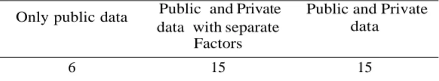
The first step of the research is to extract the factors from the public, private and the merger between public and private databases. So the first question is how many factors we should extract from each database and for that we use the Bai and Ng (2002) procedure. Table 1 presents the number of factors estimated by the Bai and Ng (2002) procedure. The procedure indicates that there are six factors for the public database (with 31 variables) and 15 factors for the private database or the merging of private and public databases. The number of factors is the same for the private database or merging with the public database.
Table 1: Number of Factors based on the Bai and Ng (2002) procedure Only public data Public and Private
data with separate Factors
Public and Private data
6 15 15
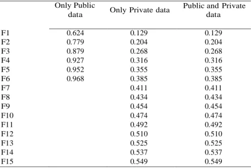
We extract the number of factors according to the procedure of Bai and Ng (2002) and the next step is to describe the percentage of the variance of the variables is related to the factors of each database. Table 2 presents the cumulative proportion of the variance of the variables which are explained by the factors together. For example, factors 1 to 6 account for 96.8% of the total variance in the case of only public data. Factor 1 explain 62.4% of the total variance in the case of only public data. However, when adding more variables with the private data, the first factor explains 12.9% of the total variance. The main concern is whether a small number of factors can account for the variability of the database. In cases of only private data or the merger of public and private data, we have factor that account for 55% of the total variance of the variables.
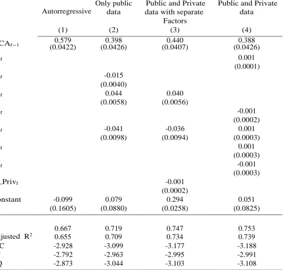
The next step is to analyze whether the factors are relevant to explain inflation and whether private information leads to gains in model adjustment. Table 3 presents the coefficients of the variables chosen by the Autometrics algorithm. We present only the coefficients of the factors and
4There is the case where the factors extracted from the database with integrated variables of order one are coin- tegrated with the variables of interest. We do not discuss this point. See for example the articles by Banerjee and Marcellino (2009) and Banerjee et al. (2014, 2015). These articles develop a factor-augmented error correction model in which the levels of a subset of the variables are cointegrated with the common factors.
Table 2: Cumulative Proportion of Variance Only Public
Only Private data Public and Private
the autoregressive terms that the Autometrics algorithm selects as relevant in table 3. The general model considers the factors extracted from each database (there are three different ways of arranging the database to extract the factors) until the second lag, the auto-regressive variables (until the second lag), the dummy variables of outlier, step and impulse. Table 5 in the Appendix shows the coefficients of the dummy variables of outlier and step that the algorithm selects as relevant.
The first column of results presents the autoregressive model with the dummy variables as bench- mark for the other results. The algorithm selects the first lag as relevant for any model considered as can be seen in Table 3. The selection through the algorithm leads to statistically significant coefficients in this case presented in Tables 3 and 5.
The Autometrics algorithm selects an autoregressive model with the dummy variables that ex- plains 66.7% of the inflation variations in column 1 of Table 3. We compare the models with factors extracted from the public and private databases in relation to the explanatory power of the autoregressive model with dummy variables for example.
Before analyzing the models with factors, we highlight that the algorithm only selects factors contemporaneously to explain inflation in either case (we allow for the second factor lag in the overall model). We extract six factors from the database with only public data. Thus, we use the algorithm to analyze whether the factors of the public database are relevant to explain inflation. Column 2 of Table 3 shows the coefficients, which indicates that the second, third and fifth factors (F2, F3 and F5) are relevant. The inclusion of factors leads to an increase in the explanatory power of the model through R2 or even considering the adjustment by the addition of explanatory variables by
adjusted R2. There is an explanation gain of 5 percentage points of inflation using the factors
extracted from the public database. In addition, the Akaike (AIC), Schwarz (SC), and Hannan- Quinn (HQ) information criteria decrease at column 2 in relation to column 1, indicating that there is an improvement of the model with factors extracted from the public database. However, the first factor is not relevant to explain inflation. That is, the factor accounting for most of the total variance of the variables in the public database is not relevant to explain inflation.
Column 3 presents the results using the factors extracted from the public and private databases separately so that we have two sets of factors, those extracted from the public database and t hose extracted from the private database. So we have the factors from the public database (F1,...,F6) and the factors from the private database (F1 Priv,...,F15 Priv). Column 3 shows that factors 3
data data F1 0.624 0.129 0.129 F2 0.779 0.204 0.204 F3 0.879 0.268 0.268 F4 0.927 0.316 0.316 F5 0.952 0.355 0.355 F6 0.968 0.385 0.385 F7 0.411 0.411 F8 0.434 0.434 F9 0.454 0.454 F10 0.474 0.474 F11 0.492 0.492 F12 0.510 0.510 F13 0.525 0.525 F14 0.537 0.537 F15 0.549 0.549
Table 3: Variable selection with the factor model (0.0001) R2 Adjusted R2 AIC -2.928 -3.099 -3.177 -3.188 SC -2.792 -2.963 -2.995 -2.991 HQ -2.873 -3.044 -3.103 -3.108
Note: the standard error of the estimated coefficients is in parentheses.
0.667 0.719 0.747 0.753
0.655 0.709 0.734 0.739
Autorregressive
Only public data
Public and Private data with separate
Factors
Public and Private data (1) (2) (3) (4) IPCAt−1 (0.0422) 0.579 (0.0426) 0.398 (0.0407) 0.440 (0.0426) 0.388 F1t 0.001 F2t -0.015 (0.0040) F3t 0.044 0.040 (0.0058) (0.0056) F4t -0.001 (0.0002) F5t -0.041 -0.036 0.001 (0.0098) (0.0094) (0.0003) F6t 0.001 (0.0003) F7t -0.001 (0.0003) F4 Privt -0.001 (0.0002) Constant -0.099 0.079 0.294 0.051 (0.1605) (0.0880) (0.0258) (0.0825)
and 5 extracted from the public database (F3 and F5) remain relevant, but factor 4 extracted from the private database (F4 Priv) is relevant additionally. Adding the set of private database factors leads to the irrelevance of the second factor in the public database. In general, in this case the factors that account for most of the total variance of the variables of each database are excluded in the explanation of inflation. The inclusion of factors from the private database leads to gains in explanatory power (through R2 or adjusted R2) and to a better model because of the lower value
for all the information criteria.
In column 4, we have the results extracting the factors from the public and private database together. Among the 15 extracted factors, the algorithm selects the first, fourth, fifth, sixth and seventh factors (F1, F4, F5, F6, and F7) as relevant. This is the only result where the first factor is relevant. The use of unified database factors increases the explanatory power of the model and we can consider as the best model by the AIC and HQ information criteria. Although the difference between extracting the factors from the public and private database separately or jointly is small.
Table 5 in Appendix presents the coefficients of dummy variables that are relevant according to the algorithm. The dummy variable for the month of June is relevant in two of the models that would be the only relevant seasonal variable in these models. The step and impulse dummy variables are relevant mainly for the years 2000, 2001, 2002 and 2018. The next step is to try to rationalize the selected dummy variables. The rationing of energy is the main event in the year 2001. The year 2002 is related to the depreciation of the nominal exchange rate due to the uncertainties arising from the Brazilian presidential election that year. The year 2018 is marked by a strike of the truck drivers due to freight and diesel prices, among other points.
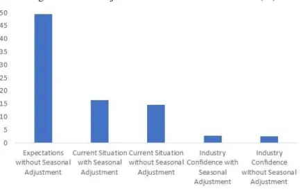
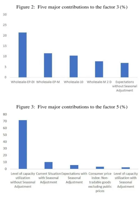
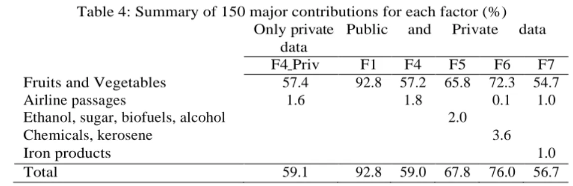
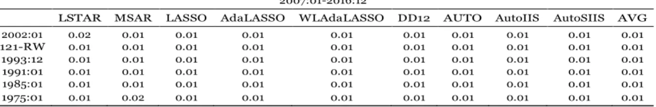
An additional step is to analyze the factors extracted from the three different databases and we analyze which variables contributed to the factor in percentage. First, we look at factors 2, 3 and 5 with the public database that the algorithm selects as relevant to explain inflation in column 2 of Table 3. Figures 1, 2 and 3 present the five main contributions, respectively, to factors 2, 3 and 5 and the percentage contribution of each indicator to the factor. Three components of the industry confidence indicator contribute to 80% of factor 2.5 The five largest contributions to factor 3 are the
wholesale price index (and its variations), which contributes by 51% only considering these five major contributions. The level of utilization of installed capacity contributes to 72% in the construction of factor 5. In other words, we can say that factors 2, 3 and 5 would be a proxy, respectively, of the industry confidence index, wholesale price index and the level of capacity utilization.
Figure 1: Five major contributions to the factor 2 (%)
5The three components of the industry confidence index are the expectations indicator (without seasonal ad - justment) and the current situation index (with and without seasonal adjustment). Only the index of expectations contributes to 49% of factor 2.
Figure 2: Five major contributions to the factor 3 (%)
Figure 3: Five major contributions to the factor 5 (%)
Table 4 presents the percentages of the groups with the 150 main contributions for each factor in cases with only the private data and merging the private and public databases. In the case of the private database (which includes only inflation price indexes), the fourth component is relevant to explain inflation. The 150 largest contributions for the construction of factor 4 represent 59.1%. Of these 59.1%, 57% are fruits and vegetables (in different price indices) and 1.64% comes from airline passages.
In the case of merging the private and public databases, the 150 largest contributions to the construction of factor 1 contribute to 93%, which are vegetables and fruits. In the case of factor 4, the 150 largest contributions to the construction of factor 4 present 59% of factor 4. Among these 59%, vegetables and fruits contribute 57% and airline passages 2%. Regarding factor 5, the 150 largest contributions for the construction of factor 5 add up to a percentage of 68%. Of these 68%, fruits and vegetables make up 66% and ethanol, sugar, biofuels and alcohol lead to 2%. Regarding factor 6, the 150 largest contributions correspond to 76% of factor 6. Among these 76%, 72% correspond to fruits and vegetables, 4% come from chemicals (ammonia, sulfuric acid, among others), kerosene and airline passages. Finally, the 150 largest contributions correspond to 57% of factor 7. Among these 57%, 55% come from fruits and vegetables, 2% from air passages and iron products. That is, the extraction of factors from the private database leads the inflation price index of fruits and vegetables to dominate the contribution to construct factors that are relevant to explain inflation.
Table 4: Summary of 150 major contributions for each factor (%) Only private
data
Public and Private data
F4 Priv F1 F4 F5 F6 F7
Fruits and Vegetables 57.4 92.8 57.2 65.8 72.3 54.7 Airline passages
Ethanol, sugar, biofuels, alcohol Chemicals, kerosene Iron products 1.6 1.8 2.0 0.1 3.6 1.0 1.0 Total 59.1 92.8 59.0 67.8 76.0 56.7
6 Conclusion
We seek to analyze whether the use of private data leads to gains in explaining Brazilian inflation between 2000 and 2018. Mainly because of the number of variables present in the private database, we need to reduce dimensionality. We choose to use the factor method to extract few factors that summarize the variables. Therefore, we use three database options to extract factors: (i) factors only from the public database, (ii) factors only from the private database, and (iii) factors from the merger of public and private databases. We determine the number of factors from the procedure of Bai and Ng (2002).
We start with an autoregressive model with two lags of the dependent variable and the factors extracted from the public and private databases, with the addition of seasonal and impulse and step dummy variables. To reduce the size of covariates, we use the Autometrics algorithm to retain the relevant covariates that explain the Brazilian inflation.
Our result is that the factors extracted from the public database bring gains to explain inflation in relation to an autoregressive model. However, the use of factors tied to the private database still leads to explanatory gains for inflation when compared to the model with only factors extracted from the public database or the autoregressive model. The gain in explanatory power for inflation when using the factors extracted from the private database is around 3 percentage points relative to using only the factors of the public database. That is, we have been able to explain about 75% of the inflation variations with the use of the factors extracted from the private and public databases. However, the algorithm does not select the first factor as relevant, except in the case where we extract the factors from the public and private databases together. This means that the factor accounting for most of the total variance of the database variables is not relevant to explain inflation unless we extract the factors from the public and private databases together.
References
F. Altissimo, A. Bassanetti, R. Cristadoro, M. Forni, M. Hallin, M. Lippi, L. Reichlin, and G. Veronese. Eurocoin: A real time coincident indicator of the euro area business cycle. Technical Report DP3108, CEPR, 2001.
F. Altissimo, R. Cristadoro, M. Forni, M. Lippi, and G. Veronese. New eurocoin: Tracking eco- nomic growth in real time. Review of Economics and Statistics, 92(4):1024–1034, nov 2010. doi: 10.1162/resta00045.
S. B. Aruoba and F. X. Diebold. Real-time macroeconomic monitoring: Real activity, inflation, and interactions. American Economic Review, 100(2):20–24, may 2010. doi: 10.1257/aer.100.2.20. S. B. Aruoba, F. X. Diebold, and C. Scotti. Real-time measurement of business conditions. Journal
J. Bai and S. Ng. Determining the number of factors in approximate factor models. Econometrica, 70 (1):191–221, jan 2002. doi: 10.1111/1468-0262.00273.
J. Bai and S. Ng. Confidence intervals for diffusion index forecasts and inference for factor -augmented regressions. Econometrica, 74(4):1133–1150, jul 2006. doi: 10.1111/j.1468-0262.2006.00696.x. M. Ban´bura, D. Giannone, M. Modugno, and L. Reichlin. Now-casting and the real-time data flow.
In G. Elliott and A. Timmermann, editors, Handbook of Economic Forecasting, volume Volume 2, chapter 4, pages 195–237. Elsevier, 2013. doi: 10.1016/b978-0-444-53683-9.00004-9.
A. Banerjee and M. Marcellino. Factor-augmented error correction models. In N. Shephard and J. Castle, editors, The Methodology and Practice of Econometrics: Festschrift in Honor of D.F.
Hendry, chapter Ch. 9, pages 227–254. Oxford University Press, 2009.
A. Banerjee, M. Marcellino, and I. Masten. Forecasting with factor-augmented error correction models.
International Journal of Forecasting, 30(3):589–612, jul 2014. doi: 10.1016/j.ijforecast.2013.01.009.
A. Banerjee, M. Marcellino, and I. Masten. An overview of the factor-augmented error correction model. In E. Hillebrand and S. Koopman, editors, Advances in Econometrics: Dynamic Factor
Models, volume 35. Emerald Group Publishing, 3–41, 2015.
B. S. Bernanke, J. Boivin, and P. Eliasz. Measuring the effects of monetary policy: A factor-augmented vector autoregressive (favar) approach. The Quarterly Journal of Economics, 120(1):387–422, 2005. R. Cristadoro, F. Mario, L. Reichlin, and G. Veronese. A core inflation indicator for the euro area.
Journal of Money, Credit and Banking, 37:539–60, 06 2005. doi: 10.1353/mcb.2005.0028.
T. M. Crone and A. Clayton-Matthews. Consistent economic indexes for the 50 states. Review of
Economics and Statistics, 87(4):593–603, nov 2005. doi: 10.1162/003465305775098242.
J. Doornik. Autometrics. In J. L. Castle and N. Shephard, editors, The Methodology and Practice
of Econometrics: Festschrift in Honor of D.F. Hendry, chapter Chap. 4, pages 88–121. Oxford
University Press, 2009.
J. A. Doornik and D. F. Hendry. Empirical Econometric Modelling - PcGive 12. Timberlake Consul- tants Ltd., 2007.
J. A. Doornik and D. F. Hendry. PcGive 13. Timberlake Consultants Press, 2009.
S. Eickmeier and C. Ziegler. How successful are dynamic factor models at forecasting output and infla - tion? a meta-analytic approach. Journal of Forecasting, 27(3):237–265, 2008. doi: 10.1002/for.1056. G. Elliott and A. Timmermann. Economic Forecasting. Princeton University Press, 2016.
L. P. Hansen and S. F. Richard. The role of conditioning information in deducing testable restrictions implied by dynamic asset pricing models. Econometrica, 55(3):587, may 1987. doi: 10.2307/1913601. D. F. Hendry and B. Nielsen. Econometric modeling: a likelihood approach. Princeton University
Press, 2007.
G. James, D. Witten, T. Hastie, and R. Tibshirani. An Introduction to Statistical Learning. Springer New York, 2013. doi: 10.1007/978-1-4614-7138-7.
S. C. Ludvigson and S. Ng. The empirical risk–return relation: A factor analysis approach73. Journal
J. Stock and M. Watson. Dynamic factor models, factor-augmented vector autoregressions, and struc- tural vector autoregressions in macroeconomics. In Handbook of Macroeconomics, pages 415–525. Elsevier, 2016. doi: 10.1016/bs.hesmac.2016.04.002.
J. H. Stock and M. W. Watson. New indexes of coincident and leading economic indicators. In O. J. Blanchard and S. Fischer, editors, NBER Macroeconomics Annual, volume Volume 4, pages 351–409. MIT Press, 1989.
J. H. Stock and M. W. Watson. A probability model of the coincident economic indicators. In K. Lahiri and G. H. Moore, editors, Leading economic indicators, pages 63–90. Cambridge University Press, 1991. doi: 10.1017/cbo9781139173735.005.
J. H. Stock and M. W. Watson. A procedure for predicting recessions with leading indicators: econo- metric issues and recent experience. In H. James and M. W. Watson, editors, Business Cycles
Indicators and Forecasting, pages 95–156. University of Chicago Press, 1993.
J. H. Stock and M. W. Watson. Forecasting inflation. Journal of Monetary Economics, 44(2):293–335, oct 1999. doi: 10.1016/s0304-3932(99)00027-6.
J. H. Stock and M. W. Watson. Macroeconomic forecasting using diffusion indexes. Journal of Business
& Economic Statistics, 20(2):147–162, apr 2002. doi: 10.1198/073500102317351921.
J. H. Stock and M. W. Watson. Dynamic factor models. In M. P. Clements and D. F. Hendry, editors,
Oxford Handbook on Economic Forecasting. Oxford University Press, jul 2011. doi: 10.1093/ox-
7 Appendix
Table 5: Dummy variables in the model
Autorregressive
Only public data
Public and Private data with separate
Factors
Public and Private data (1) (2) (3) (4) Seasonal6 -0.211 -0.182 (0.0559) (0.0506) DIS:2000(7) 1.035 (0.1884) DIS:2000(8) 0.971 (0.1855) DIS:2001(7) 0.426 (0.1428) IIS:2000(7) 0.975 1.318 (0.2119) (0.2057) IIS:2002(11) 1.364 1.389 1.359 (0.2290) (0.2162) (0.2161) IIS:2002(11) 2.041 (0.2298) IIS:2003(1) 0.814 0.753 (0.2370) (0.2179) IIS:2018(6) 1.019 0.713 0.584 (0.2330) (0.2087) (0.2002) IIS:2018(8) -0.512 (0.2004) SIS:2000(6) -1,0003 (0.2262) SIS:2000(7) 0.947 (0.2032) SIS:2001(6) -0.863 (0.2055) SIS:2001(7) 0.773 (0.1996) SIS:2018(6) 0.224 0.261 (0.0871) (0.0820) SIS:2018(10) 0.320 (0.1620)
15
it
it
Unit Root Tests for Loss Function Differentials
Tables A1-A4 show the p-value of Augmented Dickey-Fuller tests for unit roots for the loss
function differential series used in the Diebold and Mariano tests presented in Tables 4,
5, 6 and 7 in Section 5, comparing sample and methods with quadratic and absolute loss
functions.
Table A1: Augmented Dickey-Fuller Test Comparing Samples: g(e
it) = e
2.
2007:01-2016:12AR LSTAR MSAR LASSO AdaLASSO WLAdaLASSO AUTO AutoIIS AutoSIIS AVG 121-RW 0.03 0.01 0.01 0.01 0.01 0.01 0.01 0.01 0.01 0.02 1993:12 0.01 0.03 0.01 0.01 0.01 0.01 0.01 0.01 0.01 0.02 1991:01 0.01 0.01 0.01 0.01 0.01 0.01 0.04 0.01 0.01 0.01 1985:01 0.01 0.02 0.01 0.01 0.01 0.01 0.01 0.01 0.01 0.02 1975:01 0.01 0.04 0.01 0.01 0.01 0.01 0.01 0.01 0.01 0.01 Notes: ADF tests include constant and trend. g(eit) specifies the loss function used in the DM test. The
first column denotes the initial observation of the estimation sample, 121-RW denotes a 121 months rolling window forecasting scheme. Minimum p-value reported is 0.01.
Table A2: Augmented Dickey-Fuller Test Comparing Samples: g(e
it) = |e
it|.
2007:01-2016:12AR LSTAR MSAR LASSO AdaLASSO WLAdaLASSO AUTO AutoIIS AutoSIIS AVG 121-RW 0.01 0.01 0.01 0.01 0.01 0.01 0.01 0.01 0.01 0.01 1993:12 0.01 0.01 0.01 0.01 0.01 0.01 0.01 0.01 0.01 0.01 1991:01 0.01 0.01 0.01 0.01 0.01 0.01 0.10 0.01 0.01 0.01 1985:01 0.03 0.01 0.04 0.01 0.01 0.01 0.04 0.01 0.01 0.01 1975:01 0.02 0.01 0.01 0.01 0.01 0.01 0.04 0.01 0.01 0.01 Notes: see notes from Table A1.
Table A3: Augmented Dickey-Fuller Test Comparing Methods: g(e
it) = e
2.
2007:01-2016:12
LSTAR MSAR LASSO AdaLASSO WLAdaLASSO DD12 AUTO AutoIIS AutoSIIS AVG
2002:01 0.02 0.01 0.01 0.01 0.01 0.01 0.01 0.01 0.01 0.01 121-RW 0.01 0.01 0.01 0.01 0.01 0.01 0.01 0.01 0.01 0.01 1993:12 0.01 0.01 0.01 0.01 0.01 0.01 0.01 0.01 0.01 0.01 1991:01 0.01 0.01 0.01 0.01 0.01 0.01 0.01 0.01 0.01 0.01 1985:01 0.01 0.01 0.01 0.01 0.01 0.01 0.01 0.01 0.01 0.01 1975:01 0.01 0.02 0.01 0.01 0.01 0.01 0.01 0.01 0.01 0.01
Table A4: Augmented Dickey-Fuller Test Comparing Methods: g(e
it) = |e
it|.
2007:01-2016:12
LSTAR MSAR LASSO AdaLASSO WLAdaLASSO DD12 AUTO AutoIIS AutoSIIS AVG
2002:01 0.01 0.01 0.01 0.01 0.01 0.01 0.01 0.01 0.01 0.01 121-RW 0.01 0.01 0.01 0.01 0.01 0.01 0.01 0.01 0.01 0.01 1993:12 0.01 0.01 0.01 0.01 0.01 0.01 0.01 0.01 0.01 0.01 1991:01 0.01 0.01 0.01 0.01 0.01 0.01 0.01 0.01 0.01 0.01 1985:01 0.01 0.01 0.01 0.01 0.01 0.01 0.01 0.01 0.01 0.01 1975:01 0.03 0.02 0.01 0.01 0.01 0.01 0.01 0.01 0.01 0.01
Notes: see notes from Table A1.
Plots of the Forecasts
Figures A1-A6 plot the point forecasts of all models for the different estimation samples
considered. The average of all forecasts is represented by the red lines.
17
Figure A2: Point forecasts for all models for the 121 months rolling window forecasting
scheme.
Figure A4: Point forecasts for all models for the estimation samples starting in 1991:01.
19
Figure A6: Point forecasts for all models for the estimation samples starting in 1975:01.
RMSFE, MAFE and MFE Results
Table A5 provides the medians plotted in Figure 6.
Table A5: Median Values of RMSFE, MAFE and MFE by Estimation Sample
2007:01 - 2016:12
2007:01 - 2011:12
2012:01 - 2016:12
RMSFE MAFE MFE RMSFE MAFE MFE RMSFE MAFE MFE
2002:01
4.25
3.16
0.64
4.65
3.28
0.31
3.65
2.99
0.97
121-RW
3.95
3.06
0.44
4.34
3.20
0.16
3.51
2.91
0.94
∗1993:12
3.82
2.93
0.50
4.25
3.08
-0.02
∗3.40
∗2.88
∗1.10
1991:01
3.85
2.90
∗0.54
4.25
3.01
∗0.02
∗3.40
∗2.88
∗1.10
1985:01
3.94
3.09
0.44
4.12
3.08
-0.23
3.61
3.03
1.09
1975:01
3.81
∗3.00
0.38
∗4.12
∗3.03
-0.05
3.53
2.95
0.95
Notes: Median values for RMSFE, MAFE and MFE in Tables 1, 2 and 3. The first column denotes the initial observation of the estimation sample, 121-RW denotes a 121 months rolling window forecasting scheme. The first row marks the forecast horizon evaluated. Lowest absolute values in each column are marked by *.