www.atmos-chem-phys.net/8/5535/2008/ © Author(s) 2008. This work is distributed under the Creative Commons Attribution 3.0 License.
Chemistry
and Physics
Comparison of ground-based Brewer and FTIR total column O
3
monitoring techniques
M. Schneider1, A. Redondas2, F. Hase1, C. Guirado2, T. Blumenstock1, and E. Cuevas2 1IMK-ASF, Forschungszentrum und Universit¨at Karlsruhe, Karlsruhe, Germany
2Centro de Investigaci´on Atmosf´erico de Iza˜na, Agencia Estatal de Meteorolog´ıa, Spain Received: 24 September 2007 – Published in Atmos. Chem. Phys. Discuss.: 9 January 2007 Revised: 10 July 2008 – Accepted: 19 August 2008 – Published: 17 September 2008
Abstract. We compare the currently most precise, ground-based total O3 measurement techniques: Brewer and FTIR. We give an overview of the similarities and the differences between the measurements and the retrieval approaches of both experiments. We compare coincident measurements performed at the Atmospheric Observatory of Iza˜na from 2005 to 2007 and demonstrate that, if the properties of the instruments are well characterised, the scatter between both experiments is as small as 0.5%. This is in agreement with the theoretical predictions and confirms empirically that both techniques are able to monitor total O3amounts with a pre-cision of better than 0.4%. However, we found systematic differences between both techniques of around 4.5%, which we think are mainly due to discrepancies between the applied UV and infrared spectroscopic parameters.
1 Introduction
Over the last 20 years significant progress was made con-cerning the precision and accuracy of atmospheric remote sensing measurements. This development is due to improve-ments in both instrumental setups and in retrieval algorithms. High precision measurements performed on a continuous ba-sis are needed in order to detect potential atmospheric trends as soon as possible. A good example is the atmospheric ozone content. In the coming decades some kind of ozone recovery is expected, however, it is difficult to predict how, when, and to what extent it will occur (Weatherhead and An-dersen, 2006). Continuous high precision measurements of
Correspondence to:M. Schneider ([email protected])
O3are very important in this context. They provide for im-proved atmospheric O3models by detecting trends between the models and the measurements as soon as possible.
which guarantees highest quality standards. Both FTIR and Brewer activities are part of NDACC (Network for Detec-tion of Atmospheric ComposiDetec-tion Change; Kurylo (1991, 2000); http://www.ndacc.org/). Currently, such high qual-ity and continuously performed FTIR and Brewer measure-ments only coincide at the Iza˜na Observatory. Therefore, it is a predestinated site for an inter-comparison study of both techniques.
In the following we list the main similarities and differ-ences of the FTIR and Brewer technique, and discuss their respective advantages and disadvantages (Sect. 2). In Sect. 1 we briefly introduce the site where the measurements used in this work were made. In Sects. 2 to 6 we compare operational data from two different Brewer spectrometers and the FTIR spectrometer. Finally, we summarise the reasons that make the Iza˜na data unique and conclude about the implications of our results (Sects. 7 and 8).
2 FTIR versus Brewer technique
The principle of both techniques is the same: both the FTIR and the Brewer spectrometer detect direct solar light. The ex-perimental differences are the spectral regions that are anal-ysed and the spectral resolution of the measurements. The respective retrieval algorithms deduce the atmospheric O3 amounts by analysing the absorption signatures imprinted onto the extraterrestrial solar spectrum. For this purpose the Brewer and FTIR technique use different retrieval ap-proaches, which are imposed by the nature of the respective experimental data.
2.1 The experiments
The Brewer spectrometer detects spectral irradiance in six channels in the UV (303.2, 306.3, 310.1, 313.5, 316.8, and 320.1 nm) each covering a bandwidth of 0.5 nm (resolu-tion powerλ/1λof around 600). The spectral analysis is achieved by a holographic grating in combination with a slit-mask which selects the channel to be analysed by a photo-multiplier. At Iza˜na only MK-III Brewer instruments with double monochromators are applied which widely reduces the impact of straylight on the measurements. The Brewer system works in a completely automatic way, and usually measures continuously during the whole day. The first chan-nel at 303.2 nm is only used for spectral wavelength checks by means of internal Hg-lamps, the second channel is used for measuring SO2and the remaining four channels at longer wavelength determine the O3amounts. The finally reported O3result is the mean value of a set of 5 observations. The standard deviation within these 5 observations is used for the acceptance of the measurement, here we consider a mea-surement to be valid if this standard deviation is lower than 2.5 DU. The Brewer’s field of view (FOV) is about 2.7◦ (di-ameter of solar disc is 0.5◦). Consequently, all direct solar
irradiance is coupled into the spectrometer even for a mod-erate misalignment of the solar tracker. On the other hand, a certain fraction of the diffuse radiance (circumsolar) is mea-sured together with the direct irradiance. This signal of the diffuse radiance increases with the amount of scattering, i.e. mainly with SZA and aerosols, and alters the retrieved O3 amounts.
The Brewer experiment needs some instrumental charac-teristics to be determined by calibration experiments: the wavelength calibration and the slit function (instrumental line shape function), and the extraterrestrial constant (ETC). The slit function is determined once per year. This is done in a laboratory by means of low pressure discharge lamps (e.g. Fioletov et al., 2005; Gr¨obner et al., 1998). The exact wave-length settings are monitored in an automated mode every 40 min by means of the internal Hg-lamps. The slit func-tion and the exact wavelength settings are necessary to con-volve the highly resolved Bass and Paur (1985) O3 absorp-tion coefficients with the instrumental funcabsorp-tion. The ETC is the weighted sum of the logarithms of the intensity that would be detected by the different channels in the absence of any terrestrial atmosphere (according to Eq. 6 and text thereafter). The Iza˜na sky conditions allow the determina-tion of the ETC for each Brewer independently by the Lan-gley method. However, in this work we use the ETC trans-ferred by the traveling world standard Brewer #017. This ETC calibration is done once per year. The traveling world standard is applied to guarantee a world-wide consistency within the Brewer network. The stability of the ETC cali-bration is monitored continuously in an automated mode us-ing an internal halogen lamp. The difference between the weighted counts of the halogen lamp at the time of calibra-tion and the smoothed mean of two weeks is used to correct the ETC (Fioletov et al., 2005).
The mid-infrared FTIR measurement program covers the spectral region from 700 to 4200 cm−1 (corresponding to 14.3 to 2.4µm), excluding the region between 1400 and 1700 cm−1, which is not useful for ground-based measure-ments due to strong water vapour absorption. The spec-tral range is split up in 6 filter regions. For the longer wavelength region we use a band-pass filter for the 700– 1400 cm−1 region. The spectra are obtained by a Fourier analysis of the recorded interferograms. The spectral reso-lution depends on the maximum optical path difference be-tween the interfering light beams. For operational O3 mea-surements the FTIR spectra are measured with a resolution of 0.005 cm−1, which corresponds to a resolution powerλ/1λ at 1000 cm−1 of 2
allow the retrieval of a temperature profile which is expected to widely improve the precision of the retrieved total O3 amount (Schneider and Hase, 2008). It is important to men-tion that all these individual rotamen-tional-vibramen-tional lines are resolved: in the middle infrared the shape of absorption lines is dominated by pressure broadening with a typical HWHM of 0.04 cm−1 at surface level, which is nearly one order of magnitude larger than the operational resolution of the FTIR spectrometer. The numerous fine-structured spectral features provide for an automatic wavelength calibration. The FTIR spectrometer has a field of view of only 0.2◦, i.e. it only anal-yses sunlight coming from the center of the solar disc (di-ameter of 0.5◦). Consequently, a misalignment of the solar tracker directly affects the observing geometry. In Schneider and Hase (2008) it is shown that for elevation angles below 20◦ this is the leading error source. Although on a much higher level of spectral resolution if compared to the Brewer, it is important to monitor the instrumental line shape (ILS) of the FTIR spectrometer. This is done regularly by perform-ing low pressure cell calibration measurements as described in Hase et al. (1999). Even then the residual ILS error is estimated to be the most important error source concerning FTIR total O3 amounts measured at solar elevation angles above 20◦.
2.2 The retrieval approaches
The basic equation for analysing solar absorption spectra is Lambert Beer’s law:
I (λ)=IET(λ)exp(−τO3(λ)−6xτx(λ)) (1)
HereI (λ)is the measured intensity at wavelengthλ,IETthe extraterrestrial intensity,τO3the optical depth due to O3, and τxthe optical depth due to all other atmospheric components
(other trace gases, aerosols etc.). For O3it is:
τO3(λ)=
Z
σO3(λ, s)nO3(s)ds (2)
wherebyσO3(λ, s)is the absorption cross section andnO3(s)
the concentration of O3at locations. The integration is per-formed along the path of the direct sunlight. The cross sec-tionσO3depends on temperature and in the infrared
addition-ally on pressure.
The integration ofnO3 perpendicularly throughout the
at-mosphere gives the total O3column amount (O3):
O3=
Z
nO3(z)dz (3)
To deriveO3 from the measurements both techniques apply
different approaches.
2.2.1 Principles of the Brewer retrieval
The Brewer algorithm considers the absorption by O3 and SO2, scattering by molecules, and extinction by aerosols. The algorithm applies an airmass factor (µx), according to:
µx=sec
arcsin
R
R+hx
sin2
(4) as the ratio between the slant and the vertical total col-umn amount. Here R, 2, and hx are the Earth’s radius,
the apparent solar zenith angle (90◦ – elevation angle), and the effective altitude of the absorbing or scattering compo-nent (h=22 km for O3, SO2, and aerosols, and h=5 km for Rayleigh scattering). Equation (4) is a simplification of the real situation. It assumes that the absorbing compounds are concentrated at a single altitudehxand it disregards that the
refraction index depends on altitude. The errors produced by these assumptions are important for low solar elevation angles (for an elevation angle of 10◦this error is 2–3% Bern-hard et al., 2005).
Taking the logarithm of Eq. (1) and applying Eqs. (2) and (3) yields the following relation between the intensities at channeli(Ii) and the amount of the extinction components:
logIi=logIET,i−6xµxσxx−µO3σO3O3 (5)
The four channels at the longer wavelength are combined (Evans et al., 1987),
64i=1wilogIi=ETC−64i=1wi(6xµxσxx+µO3σO3O3) (6)
and the weighting coefficients wi are selected to
min-imise the influence of SO2: w[1;4]=[1.0, −0.5, −2.2, 1.7]. This choice also widely eliminates absorption fea-tures which depend in local approximation linearly on wavelength (λ) like Rayleigh scattering and aerosol extinc-tion, since64i
=1wiλi≈6 4
i=1wi=0. In Eq. (6) we replaced 6i4
=1wilogIET,i, the extraterrestrial coefficient, by ETC. With the wavelength and slit function calibration we can cal-culate the convolved extinction coefficients (σx of Eq. 6).
The ETC is transferred from a reference instrument (Fio-letov et al., 2005). Changes with time in the sensitivity of the instrument are reflected in changes of this extraterrestrial coefficient. Equation (6) together with Eq.(4) provides the total vertical O3amount. For the derivation of Eq. (5) we have to assume a constant so-called effectiveσx throughout
the atmosphere. Any temperature or pressure dependence is neglected. The “operational” algorithm applies aσO3
corre-sponding to an effective height of O3of 22 km and a fixed effective temperature of the O3layer of−45◦C. These sim-plifications produce systematic and random errors. In the case of the Iza˜na Observatory the effective height is about the same as the one used by the operational algorithm, but the ef-fective temperature ranges from−50◦C in winter months to
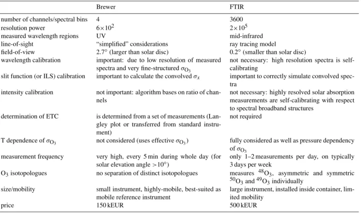
Table 1. Main differences between Brewer and FTIR experiments.
Brewer FTIR
number of channels/spectral bins 4 3600
resolution power 6×10² 2×10⁵
measured wavelength regions UV mid-infrared
line-of-sight “simplified” considerations ray tracing model
field-of-view 2.7◦(larger than solar disc) 0.2◦(smaller than solar disc)
wavelength calibration important: due to low resolution of measured
spectra and very fine-structuredσO3
not necessary: high resolution spectra is self-calibrating
slit function (or ILS) calibration important to calculate the convolvedσx important to correctly simulate convolved
spec-tra
intensity calibration not important: algorithm bases on ratio of
chan-nels
not necessary: highly resolved solar absorption measurements are self-calibrating with respect to spectral broadband structures
determination of ETC is determined from a set of measurements
(Lan-gley plot or transferred from standard instru-ment)
not required
T dependence ofσO3 not considered (uses effectiveσO3) fully considered as well as pressure dependency
ofσO3
measurement frequency very high, every 5 min during whole day (for
solar elevation angle>10◦)
only 1–2 measurements per day, on typically 3 days per week
O3isotopologues no separation of distinct isotopologues measures 48O3, asymmetric and symmetric
50O
3and49O3individually
size/mobility small instrument, highly-mobile, best-suited as
mobile reference instrument
large instrument, installed inside container, lim-ited mobility
price 150 kEUR 500 kEUR
2.2.2 Principles of the FTIR retrieval
The FTIR retrieval (PROFFIT, Hase et al., 2004) applies a precise radiative transfer model (KOPRA, H¨opfner et al., 1998; Kuntz et al., 1998; Stiller et al., 1998). KOPRA is a line-by-line model which simulates the measured spectra. It includes a ray tracing module (Hase and H¨opfner, 1999) to simulate how the solar light passes through the atmo-sphere. The model uses a discretised atmosphere (here we apply 41 levels between the Earth surface and the top of the atmosphere). The optical depth for each layer, enclosed be-tween a pair of adjacent levels, is calculated by performing the integration of Eq. (2) between two levels. The applied absorption cross sectionσ for each individual line and level are parameterised according to the HITRAN spectroscopic database (Rothman et al., 2005). The parameterisation takes care of the pressure and temperature dependency ofσ, i.e. it depends on the pressure and temperature actually present at the corresponding level. Summing up theτ values of the different layers leads to the simulated spectra at the location of the observer (combination of Eqs. 1 and 2). The radiative transfer model determines the changes in the spectral fluxes yfor a changing state vectorx. These derivatives are sam-pled in a Jacobian matrixK:
∂y=K∂x (7)
InvertingKof Eq. (7) would allow an iterative calculation of the atmospheric state from the measurement alone. However, generally the problem is under-determined, i.e. the columns ofKare not linearly independent. To overcome this problem an optimal estimation (OE) approach is applied (Rodgers, 2000): since the actual atmospheric state cannot be deter-mined unambiguously from the measurement the OE ap-proach determines the most probable state for the given mea-surement. The approach is based on the Bayesian theorem and consists in maximizing a total probability density func-tion (pdf). The total pdf is the product of two pdfs: a first, describing the probabilities of the residuals of the spectral fit, and a second, describing the a-priori known probabilities of the absorbers’ distributions.
This approach produces vertical O3 concentration pro-files (nO3(z)) for several O3isotopologues (
48O
sections we always refer to the sum of all O3isotopologues when we talk about the FTIR O3amounts.
Applying highly-resolved infrared spectra it is easy to sep-arate the extraterrestrial component from the fine-structured absorption signatures of atmospheric trace gases. In the in-frared the solar radiation is reasonably close to a black body radiation at 6000 K, i.e. it has a rather smooth dependence on wavelength. The presence of the few solar lines causes no significant problem, since they are well known (e.g. Hase et al., 2006) and fully resolved by the FTIR spectrometer.
The spectral windows applied for the FTIR retrieval con-tain many spectral bins between the fine-structured absorp-tions of atmospheric trace gases to construct an empirical background continuum.
2.3 Summary
Table 1 collects the principle differences of both techniques and resumes their respective advantages. The Brewer tech-nique depends on several calibration experiments: (a) the wavelength setting and slit function calibration. The con-volved absorption cross sections strongly depend on this cal-ibrations. (b) The transfer of the extraterrestrial constant (ETC) from the world standard Brewer. The ETC is nec-essary to separate the extraterrestrial from the atmospheric signal. Errors in the ETC add directly to the slant column amounts (see Eq. 6), i.e. they are especially important for low slant column amounts. On the other hand, every single FTIR spectrum is self-calibrating with respect to the wave-length and intensity: (a) the FTIR spectrometer fully resolves many rotational-vibrational lines, it provides for a very accu-rate and automatic wavelength calibration of the measured spectra. (b) the extraterrestrial spectrum can be easily simu-lated and there is sufficient information to derive the overall instrumental transmittance from every single measurement. Nevertheless, for high precision measurements of absorbers with sharp signatures (stratospheric absorbers), it is impor-tant to monitor the actual ILS of the FTIR instrument con-tinuously. For elevation angles above 20◦the remaining ILS uncertainties are the leading error source.
The Brewer algorithm applies the sameσO3throughout the
year and throughout the whole atmosphere. It, furthermore, assumes a O3profile where all O3is concentrated in a sin-gle layer at 22 km. The FTIR retrieval, on the other hand, takes into account the actual O3and temperature profile and applies differentσO3s and temperatures for 41 different
at-mospheric levels. This is important, sinceσO3 depends on
temperature and pressure. Furthermore, the FTIR retrieval uses a comprehensive ray tracing model.
The field-of-view of the Brewer instrument is rather large so perfect tracking is less important. However, it simultane-ously analyses a significant amount of diffuse light, which is an important error source for low elevation angles. The field-of-view of the FTIR is smaller than the solar disc. For low
elevation angles (below 20◦) the FTIR data quality depends critically on a perfectly working solar tracker.
A great advantage of the Brewer technique is that the mea-surements are performed with a very compact and mobile instrument and that all measurements including the calibra-tions are made nearly automatically. The measurements are performed continuously at many sites over the globe. For these reasons Brewer O3data are often used as reference in inter-comparison studies between different instruments and techniques, including space-based instruments. FTIR spec-trometers only have limited mobility. They are generally in-stalled inside a laboratory or a big shipping container. On the other hand, they are very versatile instruments measur-ing a great variety of atmospheric species. Concernmeasur-ing O3, the FTIR measurements allow the different isotopologues to be distinguished. FTIR measurements at Iza˜na are typically performed three times per week.
3 The Iza ˜na super-site
The Brewer and FTIR measurements are performed at the Iza˜na Observatory, which is located on the Canary Island of Tenerife, 300 km from the African west coast at 28◦18′N, 16◦29′W at 2370 m a.s.l. The Iza˜na Observatory is run by the Spanish Weather Service (Agencia Estatal de Meteo-rolog´ıa). It is a World Meteorological Organization (WMO) Global Atmospheric Watch (GAW) station of global impor-tance, and there are many different institutes from differ-ent countries involved in its manifold measuremdiffer-ent program: in-situ measurements of O3, CO2, CO, CH4, N2O, NOx, SO2, SF6, . . . , different in-situ analysers and filter radiome-ter to deradiome-termine optical, physical and chemical properties of aerosols. In March 2001 Iza˜na’s ECC-sonde, DOAS, Brewer and FTIR activities were accepted by the NDACC (Network for Detection of Atmospheric Composition Change, for-merly called NDSC: Network for Detection of Stratospheric Change Kurylo (1991, 2000); http://www.ndacc.org/).
The Brewer measurements at Iza˜na started in May 1991. Since November 2003 they represent the Regional Brewer Calibration Centre for Europe (http://www.rbcc-e.org/) of WMO/GAW (World Meteorological Organisation/Global Atmospheric Watch). This Calibration Centre is essential for a coordinated European Brewer network that is needed for both present and future consistency of ground-based to-tal ozone observations and for validation of satellite instru-ments. Furthermore, it plays an important role in the devel-opment and testing of new measurement techniques for the whole Brewer network. The Brewer data are often used as a reference for validating other ground- and satellite-based instruments.
Fig. 1. Time series of total O3as measured by the site standard Brewer #157, the traveling standard Brewer #185, and the FTIR instrument.
high resolution FTIR spectrometer commercially available. Compared to the IFS 120M it has (a) a more stable instru-mental line shape and (b) a 30% higher signal to noise ratio. In Schneider and Hase (2008) it is shown that a stable ILS is an important requisite to reach total O3 precision of bet-ter than 1–2%. To guarantee highest quality of our FTIR O3 products in this work, we only use O3amounts inverted from IFS 125HR measurements.
At the Iza˜na Observatory clean air and clear sky condi-tions are prevailing around all the year. Firstly, it is located in the region below the descending branch of the Hadley cell, typically above a stable inversion layer. Secondly, it is sit-uated on an island far away from any significant industrial activities. Consequently it offers excellent conditions for at-mospheric observations by remote sensing techniques and it is predestinated for calibration and validation activities. Due to its geographic location it is in particular valuable for the investigation of stratosphere-troposphere exchange associ-ated with the subtropical jet (e.g. Kowol-Santen et al., 1999; Cuevas et al., 2007) and large scale transport from the tropics to higher latitudes.
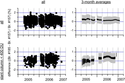
Figure 1 shows the evolution of the total O3 amounts in 2005 and 2006 as measured by the site standard Brewer #157,
Fig. 2. Correlation between total column amounts of Brewer #157 and Brewer #185. Black circles are individual measurements, red line represents linear regression line of least squares fit.
traveling standard Brewer #185, and the FTIR instrument. The Brewer #185 started its operation in April 2005. Further gaps in the time series of the Brewer data are mainly due to intercomparison campaigns of the traveling standard Brewer #185: in September it was in Huelva, Spain; in March/April 2006 and January/February 2007 in Sodankyl¨a, Finland. The gap in December 2005 is due to the (sub-)tropical storm Delta, which hit the island on 28 November. Peak gusts around 250 km/h were measured on this day and the Brewer #157 suffered some damage and was out of operation dur-ing the whole month of December 2005. Other gaps are due to power breakdown after snow storms in winter. The FTIR measures typically three times per week. The gap in Febru-ary 2005 and the relatively sparse data in winter 2006 are due to snow storms or bad weather conditions.
4 Brewer #157 versus Brewer #185
Fig. 3. Time series for the differences of total O3measured by the Brewer #157 and the Brewer #185((#185–#157)/#157). Upper panels: for all coinciding measurements; bottom panels: for measurements with low slant columns (<400 DU). The left panels show all individual coincidences and the right panels the statistics of three month averages: the black shaded area covers the range within which the mean value is situated with a probability of 95%; the grey-shaded area indicates the standard deviation. The scale of the y-axis of the right panels is expanded by a factor 2.
Fig. 4.Differences of total O3measured by the Brewer #157 and the Brewer #185 ((#185–#157)/#157) versus slant column amount. Upper
panel: for measurements between April and November 2005; bottom panel: for measurements between December 2005 and January 2007. The left panels show all individual coincidences and the right averages over values within a radius of 12.5% of the slant column amount: the black shaded area covers the range within which the mean value is situated with a probability of 95%; the grey-shaded area indicates the standard deviation. The scale of the y-axis of the right panels is expanded by a factor 2.
4.1 Temporal evolution
In the following we investigate how the difference between both Brewers evolves with time. The left panels of Fig. 3 depict the difference for all individual coincidences versus time. When contemplating this plot it is important to note
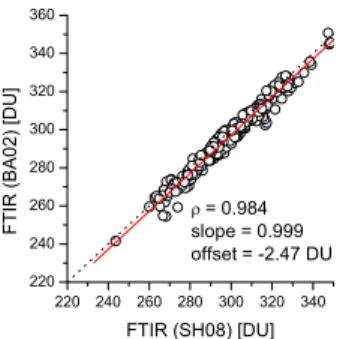
Fig. 5. Correlation between total column amounts for different FTIR approaches (a first similar to Barret et al. (2002) and a second according to Schneider and Hase, 2008). Black circles are the in-dividual measurements, the red line is the linear regression lines of the least squares fit.
we apply data within a radius of 1.5 month around the con-sidered date. The statistics of such averaged data are shown in the right panels. The grey bars represent the standard de-viation (std) of the 3-month ensembles. They can be inter-preted as overall precision of Brewer #157 and #185 within a three month period. The black bars represent the 95% con-fidence interval. This interval represents the area where the real mean value of a 3-month ensemble is situated with a probability of 95%. The radius of this area is approximately 2×√std
n (n is the number of ensemble members). Often
std √
n
(the standard error of the mean) is used to determine the con-fidence radius. However, a so-calculated area would only contain the real mean with a probability of 68%. The upper panels show the situation if all 4300 coinciding Brewer mea-surements are applied. In this case even for the three month averages there is no significant temporal variation of the dif-ference between the two Brewers. It seems that both instru-ments produce very consistent data even over several years. A small difference between 2005 and 2006 is that the over-all precision of Brewer #157 and #185 for 3 month periods is slightly better in 2006 compared to 2005 (0.4% compared to 0.5%; see grey bars).
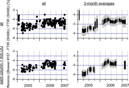
In addition we perform a separate analysis for low slant column amounts. This is done for two reasons: (1) FTIR measurements are generally performed at relatively low slant column amounts (75% of all FTIR measurements are at solar elevation angles above 35◦). On the other hand, Brewer mea-surements are performed during the whole day, and thus, Brewer data include many O3 amounts deduced from high slant column amounts. The separate analysis of low slant column assures that the Brewer data are characterised un-der similar condition as the FTIR data. (2) Systematic ETC errors are amplified for low slant column amounts, since a systematic error in the ETC produces a systematic bias in the retrieved slant column amounts (see Eq. 6). The bottom panels of Fig. 3 shows data only if the respective measure-ment was made for a slant column lower than 400 DU. This
slant column amount corresponds to an solar elevation angle of typically above 50◦. Consequently, even at the subtrop-ical site of Iza˜na, these data are not available in winter and the time series is limited to data from February to November. In these graphs we can observe a slight difference between 2005 and 2006. In 2005 both Brewers measure nearly the same, whereas in 2006 the site standard Brewer #157 pro-duces O3 amounts, which are around 0.5% lower than the Brewer #185 amounts. This observation is robust since it is based on more than 700 coincidences between the Brewers. The areas where the mean difference is situated with a prob-ability of 95% (indicated by black bars in the left panels of Fig. 3) are separated for the years 2005 and 2006: we observe a slight systematic difference in the Brewers’ performance between 2005 and 2006.
4.2 Dependence on slant column amounts
5 FTIR (Barret et al., 2002) versus FTIR (Schneider and Hase, 2008)
In this Section we compare total O3 data from two differ-ent FTIR retrieval approaches: first, using a method similar to Barret et al. (2002) (in the following called BA02) and second, similar to Schneider and Hase (2008) (in the fol-lowing called SH08). By this means we perform an inter-nal consistency check of the FTIR data. Figure 5 shows the correlation between the two approaches. Both retrievals ap-ply the same O3absorption signatures but slightly different retrieval strategies. The first consists in an optimal estimation of O3profiles alone and the second in an joint optimal esti-mation of O3,50O3/48O3, and temperature profiles. A corre-lation coefficient of “only” 0.984 is relatively low. The agree-ment is poorer if compared to the agreeagree-ment between both Brewer instruments. This is mainly due to errors from the BA02 method. In Schneider and Hase (2008) it was shown that the SH08 approach provides for significantly more pre-cise data than the BA02 approach. It nearly eliminates the error due to uncertainties in the applied temperature profiles, which are the dominant error source of the BA02 approach. On the other hand, the SH08 approach is more sensitive to errors due to ILS uncertainties (Schneider and Hase, 2008). By comparing the data of both approaches we expect to get some information about the stability of the ILS from 2005 to 2007.
5.1 Temporal evolution
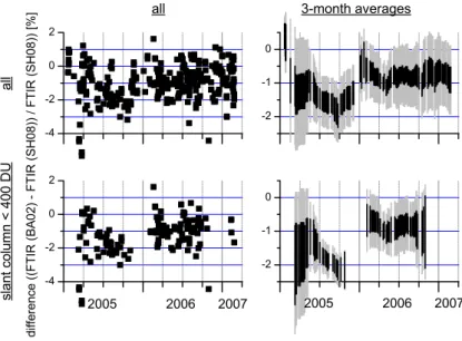
The temporal evolution of the difference between the two FTIR retrieval approaches is depicted in Fig. 6. Like for Fig. 3 the left panels show the individual measurements and the right panels show the statistics for the 3-month averages: the black bars represent the range of the mean values at a 95% confidence level, the grey bars represent the standard deviation. The upper panels show all data and the bottom panels only data for slant column amounts below 400 DU. First of all there is much more noise on the data when com-pared to Fig. 3. The relatively large noise is mainly due to temperature errors present in the BA02 approach. Again it should be remarked that the BA02 approach does not fully exploit the potential of the FTIR measurements. It is not an optimised approach, but we can exploit its different ILS sen-sitivity to perform an internal estimation of the FTIR’s ILS characterisation. This internal estimation is achieved by av-eraging over a certain amount of data. This process signifi-cantly reduces the temperature error, which is mainly a ran-dom error. The remaining systematic signal should then be due to a systematic error source, for which both retrieval ap-proaches have different sensitivities: e.g. the ILS error. The statistics of 3-month averages are depicted in the right pan-els of Fig. 6. We observe some systematic differences be-tween the years 2005 and 2006/2007. First, the year 2005 is much more variable, which may indicate that the ILS of the
FTIR instrument is less stable than in 2006/2007. Second, the difference between both approaches is larger in 2005 than in 2006/2007 (1.5% compared to 0.8%). Assuming that the amplitude of the difference follows the amplitude of the re-maining ILS error means that in 2005 the ILS is less well characterised than in 2006/2007. The bottom right panel of Fig. 6 shows the situation for slant column amounts below 400 DU. Here the differences are especially large in October 2005 (up to 2.2%). Furthermore, we observe that the dif-ference increases from April to October 2005. We think that these observations indicate a gradual decrease of the ILS per-formance during 2005.
There are several possible explications for the relatively poor instrumental stability in 2005. In January 2005, af-ter the installation of the instrument, the ILS was very well characterised (difference between BA02 and SH08 data of 0%). However, in the following there was a sequence of experimental complications. The setting of the ground or the whole surface below the container may have still been in progress during the first months of the measurements. In February 2005 there was a snow storm in Iza˜na and a subse-quent breakdown of the power supply for several days. As a consequence the temperature in the container decreased to around 0 C◦. These mechanical and thermal stresses may have produced a degradation of the optical alignment. Fur-thermore, the low temperature damaged the hygroscopic en-trance windows which had to be replaced. Unfortunately we only performed two independent ILS calibration measure-ments between January and November 2005. This is defini-tively not sufficient for a high quality characterisation of the ILS, in particular if we consider the aforementioned adverse conditions. In November 2005 we installed new firmware and reinstalled the detectors for technical servicing. The lat-ter significantly reduced a channeling of 0.58 cm−1. Since December 2005 the instrument is operating continuously and there were no further modifications necessary. In particular there was no further significant temperature breakdown in-side the measurement container. Since the end of 2005 it is kept continuously at 22 C◦.
5.2 Dependence on slant column amounts
Fig. 6. Time series for the differences between the different FTIR approaches (FTIR (BA02)–FTIR (SH08))/FTIR (SH08)). Content of panels, symbols, and colours is the same as in Fig. 3.
Fig. 7. Differences of total O3measured by the different FTIR approaches (FTIR (BA02)–FTIR (SH08))/FTIR (SH08)) versus slant column
amounts. Content of panels, symbols, and colours is the same as in Fig. 4.
6 Brewer versus FTIR
In this section we compare total O3measurements of Brewer and FTIR. To exclude influences due to temporal variabil-ities we require that both Brewer and FTIR measurements should coincide within 30 min. Between January 2005 and February 2007 we identified a total of 305 FTIR measure-ments which fulfill these coincidence criteria with the Brewer measurements: 240 for the Brewer #157, 165 for the Brewer #185. Both Brewer instruments measure generally during the whole day. Figure 8 depicts the correlation between the site standard Brewer #157 and the FTIR O3amounts. Within all
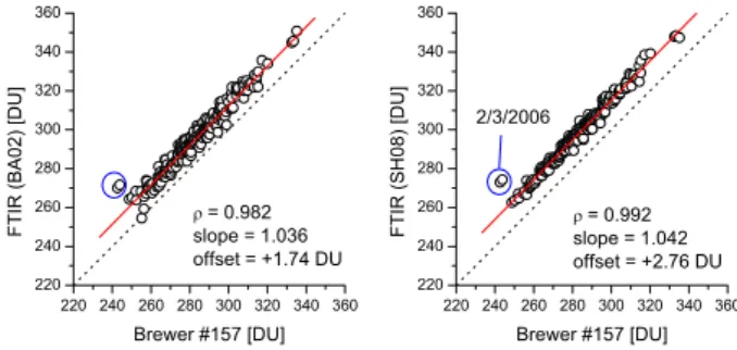
Fig. 8. Correlation between total column amounts of Brewer #157 and FTIR. Black circles are individual measurements, red lines lin-ear regression lines of least squares fits. Left panel: correlation between Brewer and BA02 FTIR retrieval; right panel: correlation between Brewer and SH08 FTIR retrieval.
and FTIR measurements performed at Iza˜na. In particular, it confirms the potential of the FTIR technique when the in-strumental aspects of the recipe as presented in Schneider and Hase (2008) are considered.
However, there is still a large potential to further improve the agreement. As shown in Schneider and Hase (2008) the BA02 error budget is dominated by errors in the assumed temperature profiles and applying the SH08 approach should widely reduce the overall FTIR errors. The correlation of the FTIR SH08 data with the Brewer #157 data is shown in the right panel of Fig. 8. It yields a correlation coeffi-cient of 0.992. The difference between both instruments is 4.9±0.7%. The SH08 data agree significantly better with the Brewer data than the BA02 data. If we only correlate Brewer and FTIR SH08 data measured after November 2005 we get an even larger improvement. Then the correlation co-efficient for the SH08 approach is 0.996 and the difference
−4.7±0.5%, whereas the BA02 approach only yields a cor-relation coefficient of 0.984 and a difference of−4.0±1.0% (Fig. 9). Limiting the comparison to measurements taken after November 2005 is justified since in 2005 the FTIR in-strument is not optimally characterised (see Figs. 6 and 7 and discussion in Sect. 5).
The data measured after November 2005 reveal the real potential of the FTIR technique. Then the scatter between the FTIR (SH08) and the Brewer data is only 0.5%. This is an excellent value for two independent remote sensing exper-iments performed over more than 1 year. It can be interpreted as the root-square-sum of the precisions of the Brewer and FTIR instrument. As aforementioned the Brewer precision is not better than 0.3%. Consequently the Brewer/FTIR com-parison is the empirical proof that the ground-based FTIR technique has the potential to measure O3 amounts with a precision of better than 0.4%. For the BA02 approach the agreement does not improve significantly if we limit the com-parison to data measured after November 2005. These data are dominated by errors caused by the assumed temperature
Fig. 9. Same as Fig. 8 but only applying data from December 2005 onward.
profiles, which are much larger than the errors caused by in-consistencies in the instrument’s performance.
The Brewer-FTIR comparison confirms the theoretical prediction of Schneider and Hase (2008). However, there are significant systematic differences between both datasets: the FTIR observing system measures systematically 4.7% more O3 than the Brewer system. These systematic differences may be due to incorrect characterisations of the instruments, simplifications in the Brewer retrieval algorithm, or discrep-ancies between the applied infrared (Rothman et al., 2005) and UV spectroscopic parameters (Bass and Paur, 1985).
Fig. 10. Time series for the differences of total O3measured by the Brewer #157 and the FTIR. ((#157–FTIR)/FTIR). Content of panels,
symbols, and colours is the same as in Fig. 3.
Fig. 11. Time series for the differences of total O3measured by the Brewer #185 and the FTIR. ((#185–FTIR)/FTIR). Content of panels,
symbols, and colours is the same as in Fig. 3.
Finally, Fig. 11 depicts the temporal evolution of the dif-ference between Brewer #185 and FTIR. As before, we ob-serve a clear difference between 2005 and 2006. In 2005 the FTIR measures typically around 5.5% larger amounts than the Brewer #185. In 2006 the difference reduces to typically 4.8%. An interesting detail of Figs. 10 and 11 is the ten-dency to increased differences in the summer months (July and August). In summer 2005 there is a kind of intermission in the trend towards reduced Brewer-FTIR differences and in summer 2006 the difference is temporarily more negative than in April or October of the same year. This feature may be produced by the Brewer algorithm’s assumption of a fixed effective O3temperature (see end of Sect. 2.2.1).
6.1 Temporal evolution
Fig. 12. Differences of total O3measured by the Brewer #157 and the FTIR. ((#157–FTIR)/FTIR) versus slant column amounts. Content
of panels, symbols, and colours is the same as in Fig. 4.
Fig. 13. Differences of total O3measured by the Brewer #185 and the FTIR. ((#185–FTIR)/FTIR) versus slant column amounts. Content
of panels, symbols, and colours is the same as in Fig. 4.
(K. Lamb, private communication) and is due to the inter-nal filters applied by the Brewer instrument. There are five grey filters assuring that an adequate light intensity enters the photomultiplier (filter #1 is weakly attenuating and filter #5 is strongly attenuating). The problem is that these filters are not ideal grey filters, i.e. their attenuation depends weakly on wavelength. This not ideal attenuation is different for each filter and causes a filter dependent error in the retrieved O3 amounts. The Brewer #185 is more sensitive than the Brewer #157. Even at large solar elevation angles the filter #3 is suffi-ciently attenuating for the Brewer #157, whereby the Brewer #185 frequently needs to switch between filter #3 and #4,
which is the reason for the elevated noise in the Brewer #185 data. It is possible to reduce this noise by correcting the er-ror caused by the not ideal grey filters. This correction is not part of the standard retrieval algorithm, and thus not ap-plied for the here presented data. The correction would also reduce the systematic difference of (Brewer-FTIR)/FTIR by 0.5% (to around−4% in 2006/2007).
6.2 Dependence on slant column amounts
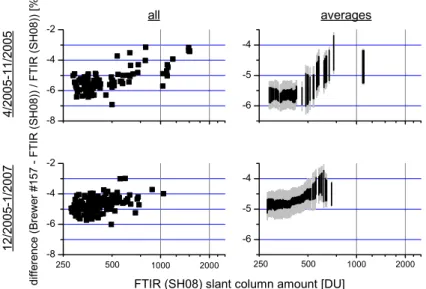
between January 2005 and November 2005. For increas-ing slant column amounts we observe a clear increase of the Brewer #157 O3amounts with respect to the FTIR amounts. At low slant columns the Brewer measures amounts which are 5.6% lower than the FTIR amounts. For slant column amounts at 700 DU this difference reduces to 4.4%. For the 2006 period the dependence on the slant column amount is less pronounced: at 700 DU the difference is around 4.5% and below 450 around 4.8%. This means that the FTIR and Brewer #157 data are more consistent in 2006 than in 2005. The upper right panel of Fig. 12 has significant similarities with the upper right panel of Fig. 7. This suggests that in 2005 the inconsistencies between the FTIR and Brewer #157 are mainly due to errors in the FTIR data.
Figure 13 shows the same as Fig. 12 but for the difference between FTIR and Brewer #185. We also found that depen-dence on slant column amounts is larger in 2005 if compared to 2006.
7 Some remarks on the quality of Iza ˜na’s O3
measure-ments
Many other observatories could reach a similar precision as Iza˜na, but there is, to our knowledge, currently world-wide no other site where total O3column amounts are measured si-multaneously by different ground-based techniques with the same high precision as presented in this work. The reasons for the currently unique high quality of the Iza˜na O3 data are manifold: (a) the outstanding meteorological conditions that prevail at the Iza˜na Observatory benefit the quality of the FTIR measurements. There are only negligible inten-sity fluctuations while recording an FTIR interferogram. At less favorable measurement sites these fluctuations are larger due to changes of the atmospheric transparency (caused by clouds, short-scale inhomogeneities in water vapour, tropo-spheric aerosols, contrails etc.). These fluctuations are gen-erally neglected, which produces errors in the retrieved O3 amounts. To achieve an excellent FTIR data quality at less favorable sites the impact of the intensity fluctuations has to be reduced. Keppel-Aleks et al. (2007) describes a method to do so. (b) The application of state-of-the-art instrumentation. The Brewer triad is formed by three state-of-the-art instru-ments with double monochromator. Intercomparison studies with single monochromator instruments indicate a signifi-cantly poorer Brewer precision (Fioletov et al., 2005). The FTIR system consist of a very precise solar tracker (Hus-ter, 1998), a Bruker IFS 125HR (stable ILS), and applies photo-voltaic detectors. These are the most important instru-mental requirements needed for high precision FTIR mea-surements. Instabilities in the ILS are one of the dominant remaining error sources. These instabilities are responsible for the internal FTIR inconsistencies observed during 2005. (c) The high precision of both Brewer and FTIR depends on regularly performed calibration measurements. In case of the
Brewer, the ETC and wavelength are monitored internally by calibration lamps several times per day. Once per year the ETC is transferred from the traveling world standard Brewer. The slit function remains very stable. It is measured every year. In case of the FTIR, regularly performed ILS calibra-tion measurements (Hase et al., 1999) are important. Since November 2005 these measurements are performed every 2– 3 months. (d) Finally, it is important to apply an optimised retrieval algorithm: the FTIR only reaches a precision better than 0.5% if the retrieval strategy as proposed by Schneider and Hase (2008) is applied.
8 Summary and conclusions
The operational Brewer data presented here are very consis-tent over more than two years. Although, in 2005 the ETC determined for the Brewer #157 seems to be slightly less ac-curate than in 2006. However, these errors are very small and are in agreement with the expected ETC uncertainties. State-of-the-art Brewer instruments (double monochromator) com-bine high precision, stability, and mobility. They are per-fectly suited for calibrating O3instruments at different sites. Furthermore, Brewer spectrometers are relatively economic and measure O3 throughout the day and during the whole year.
The FTIR data presented here can be classified in two groups. A first group consisting of the data measured in 2005, when the instrument was not optimally characterised, and a second group consisting of the data measured after November 2005. The internal consistency check of Sect. 5 reveals the problems in 2005. The strong slant column de-pendence of the difference between the two FTIR retrieval approaches (Fig. 7) indicates the non optimal characterisa-tion of the FTIR instrument. In 2005 the FTIR data do not represent the real potential of the FTIR technique. But even then we found a very small scatter with respect to the Brewer data of 0.8%. Since December 2005 the FTIR in-strument is very well characterised. Then the scatter with respect to the Brewer data is only 0.5%, which confirms the prediction of Schneider and Hase (2008). This supports the theoretical quality assessments of other FTIR products, for which no direct empirical verification can be achieved. We think that our results are of particular interest in the context of ground-based high precision measurements of greenhouse gases, which are performed within TCCON (Washenfelder et al., 2006) and will serve for the validation of OCO (Crisp et al., 2004). TCCON aims for a precision of 0.1% in the O2 corrected CO2column.
We find a significant systematic difference between the FTIR and Brewer data of 4–5%. Concerning the FTIR, a wrong ILS characterisation could produce a systematic error. This is the case in 2005, when an incorrect ILS produces an overestimation of the FTIR O3amounts of up to 1%. Con-cerning the Brewer, uncertainties in the ETC and slit function calibration or not ideal filters introduce systematic errors. An incorrect Brewer ETC assumptions as well as a wrong FTIR ILS characterisation would depend on the observed slant col-umn amount. Such a dependence is clearly observed in 2005 but only very small in 2006 and 2007. Consequently, we con-clude that the 2006/2007 data are less affected by systematic errors of instrumental nature. However, 0.5% of the differ-ence of 4.5% as observed in 2006/2007 is caused by the non ideal internal Brewer filters (see end of Sect. 6.1). We think that in 2006/2007 in the worst case 1% of the observed sys-tematic difference is due to errors in the assumed ILS, ETC, or non ideal filters. The rest is caused by the spectroscopic parameters. Our work indicates a systematic inconsistency between the infrared and UV spectroscopic coefficients of (4±1)%. This observation is in good agreement to the labo-ratory study of Picquet-Varrault et al. (2005).
For the study of the expected O3recovery, measurements which maintain a high precision over long time scales are needed. But even for regularly and carefully calibrated in-struments small instrumental drifts may occur. In this context super-sites like Iza˜na are very important. The combination of different high quality experiments (like Brewer and FTIR) at a single site makes both experiments much more valuable for trend studies as if they were performed individually at differ-ent sites: the possibility to continuously inter-compare both techniques significantly reduces the risk of detecting artificial trends that may be caused by small instrumental drifts.
Acknowledgements. We would like to thank the European Com-mission and the Deutsche Forschungsgemeinschaft for funding via the projects GEOMON (contract GEOMON-036677) and RISOTO
(Gesch¨aftszeichen SCHN 1126/1-1), respectively. Furthermore,
we are grateful to the Goddard Space Flight Center for providing the temperature and pressure profiles of the National Centers for Environmental Prediction via the automailer system. The Global Atmospheric Watch (GAW) Regional Brewer Calibration Center for Europe (RBBCC-E) is supported and maintained by the Spanish Agencia Estatal de Meteorolog´ıa (AEMet). C. Guirado has enjoyed a grant from the AEMet (Resoluci´on de 10-10-2006; BOE no. 279; 22-11-2006) at the Centro de Investigaci´on Atmosf´erico de Iza˜na.
Edited by: A. Richter
References
Barret, B., De Mazi`ere, M., and Demoulin, P.: Retrieval and char-acterization of ozone profiles from solar infrared spectra at the Jungfraujoch, J. Geophys. Res., 107, 4788–4803, 2002. Bass, A. M. and Paur, R. J.: The ultraviolet cross-sections of ozone,
I. The measurements, in: Atmospheric Ozone: Proceedings of the Quadrennial Ozone Symposium Held in Halkidiki, Greece, 3–7 September 1984, edited by: Zerefos, C. S. and Ghazi, A., Springer, New York, 606–610, 1985.
Bernhard, G., Evans, R. D., Labow, G. J., and Oltmans, S. J.: Bias in Dobson total ozone measurements at high latitudes due to approximations in calculations of ozone absorption coefficients and air mass, J. Geophys. Res., 110, D10305, doi:10.1029/2004JD005559, 2005.
Crisp, D., Atlas, R. M., Breon, F.-M., Brown, L. R., Burrows, J. P., Ciais, P., Connor, B. J., Doney, S. C., Fung, I. Y., Jacob, D. J., Miller, C. E., O’Brien, D., Pawson, S., Randerson, J. T., Rayner, P., Salawitch, R. J., Sander, S. P., Sen, B., Stephens, G. L., Tans, P. P., Toon, G. C., Wennberg, P. O., Wofsy, S. C., Yung, Y. L., Kuang, Z., Chudasama, B., Sprague, G., Weiss, B., Pollock, R., Kenyon, D., and Schroll, S.: The orbiting carbon observatory (OCO) mission, Adv. Space Res., 34, 700–709, 2004.
Cuevas, E., Rodr´ıguez, J. J., Gil, M., Guerra, J. C., Redondas, A., and Bustos, J. J.: Stratosphere-troposphere exchange processes driven by the subtropical jet, 7th EMS Annual Meeting/8th ECAM, EMS7/ECAM8 Abstracts, 4, EMS2007-A-00452, 2007. Evans, W. F. J., Fast, H., Forester, A. J., Henderson, G. S., Kerr, J. B., Vupputori, R. K. R., and Wardle, D. I.: Stratospheric ozone science in Canada: An agenda for research and moni-toring, Internal Rep. ARD-87-3, Atmospheric Environment Ser-vice, Toronto, Ontario, Canada, 128 pp., 1987.
Fioletov, V. E., Kerr, J. B., McElroy, C. T., Wardle, D. I., Savastiouk, V., and Grajnar, T. S.: The Brewer refernce triad, Geophys. Res. Lett., 32, L20805, doi:10.1029/2005GL024244, 2005.
Gr¨obner, J., Wardle, D. I., McElroy, C. T., and Kerr, J. B.: Investiga-tion of the wavelength accuracy of Brewer spectrophotometers, Appl. Optics, 37, 8352–8360, 1998.
Hase, F. and H¨opfner, M.: Atmospheric raypath modelling for ra-diative transfer algorithms, Appl. Optics, 38, 3129–3133, 1999. Hase, F., Blumenstock, T., and Paton-Walsh, C.: Analysis of the
instrumental line shape of high-resolution Fourier transform IR spectrometers with gas cell measurements and new retrieval soft-ware, Appl. Optics, 38, 3417–3422, 1999.
Hase, F., Hannigan, J. W., Coffey, M. T., Goldman, A., H¨opfner, M., Jones, N. B., Rinsland, C. P., and Wood, S. W.: Intercompar-ison of retrieval codes used for the analysis of high-resolution, ground-based FTIR measurements, J. Quant. Spectrosc. Ra., 87, 25–52, 2004.
Hase, F., Demoulin, P., Sauval, A. J., Toon, G. C., Bernath, P. F., Goldman, A., Hannigan, J. W., and Rinsland, C. P.: An empirical line-by-line model for the infrared solar transmittance spectrum
from 700 to 5000 cm−1, J. Quant. Spectrosc. Ra., 102, 450–463,
2006.
Huster, S. M.: Bau eines automatischen Sonnenverfolgers f¨ur bo-dengebundene IR-Absorptionmessungen, Diplomarbeit im Fach Physik, Institut f¨ur Meteorologie und Klimaforschung, Univer-sit¨at Karlsruhe und Forschungszentrum Karlsruhe, 1998. Keppel-Aleks, G., Toon, G. C., Wennberg, P. O., and Deutscher,
N. M.: Reducing the impact of source brightness fluctuations on spectra obtained by FTS, Appl. Optics, 46, 4774–4779, 2007. Kowol-Santen, J., Ancellet, G., and Cuevas, E.: Analysis of
Trans-port Across the Subtropical Tropopause, Proceedings for Fifth European Symposium on Stratospheric Ozone, St Jean de Luz (France), 27 September to 1 October 1999, p. 522, 1999. Kuntz, M., H¨opfner, M., Stiller, G. P., Clarmann, T. V., Echle, G.,
Funke, B., Glatthor, N., Hase, F., Kemnitzer, H., and Zorn, S.: The Karlsruhe optimized and precise radiative transfer algorithm, Part III: ADDLIN and TRANSF algorithms for modeling spec-tral transmittance and radiance, SPIE Proceedings 1998, 3501, 247–256, 1998.
Kurylo, M. J.: Network for the detection of stratospheric change (NDSC), SPIE Proceedings 1991, Remote Sensing of Atmo-spheric Chemistry, 1491 168–174, 1991.
Kurylo, M. J. and Zander, R.: The NDSC – Its status after 10 years of operation, Proceedings of XIX Quadrennial Ozone Sympo-sium, Hokkaido University, Sapporo, Japan, 167–168, 2000. Picquet-Varrault, B., Orphal, J., Doussin, J.-F., Carlier, P., and
Flaud, J.-M.: Laboratory Intercomparison of the Ozone
Absorp-tion Coefficients in the Mid-infrared (10µm) and Ultraviolet
(300–350 nm) Spectral Regions, J. Phys. Chem. A, 109, 1008– 1014, 2005.
Redondas, A. and Cede, A.: Brewer algorithm sensitivity analy-sis, SAUNA workshop, Puerto de la Cruz, Tenerife, November, 2006.
Rodgers, C. D.: Inverse Methods for Atmospheric Sounding: The-ory and Praxis, World Scientific Publishing Co., Singapore, ISBN 981-02-2740-X, 2000.
Rothman, L. S., Jacquemart, D., Barbe, A., Benner, D. C., Birk, M., Brown, L. R., Carleer, M. R., Chackerian Jr., C., Chance, K. V., Coudert, L. H., Dana, V., Devi, J., Flaud, J.-M., Gamache, R. R., Goldman, A., Hartmann, J.-M., Jucks, K. W., Maki, A. G., Mandin, J.-Y., Massie, S. T., Orphal, J., Perrin, A., Rinsland, C. P., Smith, M. A. H., Tennyson, J., Tolchenov, R. N., Toth, R. A., Vander Auwera, J., Varanasi, P., and Wagner, G.: The HI-TRAN 2004 molecular spectroscopic database, J. Quant. Spec-trosc. Ra., 96, 139–204, 2005.
Schneider M., Blumenstock, T., Hase, F., H¨opfner, M., Cuevas, E., Redondas, A., and Sancho, J. M.: Ozone profiles and total col-umn amounts derived at Iza˜na, Tenerife Island, from FTIR solar absorption spectra, and its validation by an intercomparison to ECC-sonde and Brewer spectrometer measurements, J. Quant. Spectrosc. Ra., 91, 245–274, 2005.
Schneider, M. and Hase, F.: Technical Note: Recipe for continuous monitoring of total ozone with a precision of 1 DU applying mid-infrared solar absorption spectra, Atmos. Chem. Phys., 8, 63–71, 2008,
http://www.atmos-chem-phys.net/8/63/2008/.
Stiller, G. P., H¨opfner, M., Kuntz, M., Clarmann, T. v., Echle, G., Fischer, H., Funke, B., Glatthor, N., Hase, F., Kemnitzer, H., and Zorn, S.: The Karlsruhe optimized and precise radiative trans-fer algorithm, Part I: Requirements, justification and model error estimation, SPIE Proceedings 1998, 3501, 257–268, 1998. Van Roozendael, M., Peeters, P., Roscoe, H. K., De Backer,
H., Jones, A. E., Bartlett, L., Vaughan, G., Goutail, F., Pom-mereau, J.-P., Kyro, E., Wahlstrom, C., Braathen, G., and Simon, P. C.: Validation of Ground-Based Visible Measurements of To-tal Ozone by Comparison with Dobson and Brewer Spectropho-tometers, J. Atmos. Chem., 29, 55–83, 1998.
Weatherhead, E. C and Andersen, S. B.: The search for signs of recovery of the ozone layer, Nature, 441, 39–45, 2006.