Consumer-resource dynamics: quantity, quality, and allocation.

(1)

Allocation

Wayne M. Getz1,2*, Norman Owen-Smith3

1Department of Environmental Science, Policy and Management, University of California, Berkeley, California, United States of America,2Stellenbosch Institute for Advanced Study (STIAS), Wallenberg Research Centre at Stellenbosch University, Stellenbosch, South Africa,3School of Animal, Plant and Environmental Sciences, University of the Witwatersrand, Wits, South Africa

Abstract

Background:The dominant paradigm for modeling the complexities of interacting populations and food webs is a system of coupled ordinary differential equations in which the state of each species, population, or functional trophic group is represented by an aggregated numbers-density or biomass-density variable. Here, using the metaphysiological approach to model consumer-resource interactions, we formulate a two-state paradigm that represents each population or group in a food web in terms of both its quantity and quality.

Methodology and Principal Findings:The formulation includes an allocation function controlling the relative proportion of extracted resources to increasing quantity versus elevating quality. Since lower quality individuals senesce more rapidly than higher quality individuals, an optimal allocation proportion exists and we derive an expression for how this proportion depends on population parameters that determine the senescence rate, the per-capita mortality rate, and the effects of these rates on the dynamics of the quality variable. We demonstrate that oscillations do not arise in our model from quantity-quality interactions alone, but require consumer-resource interactions across trophic levels that can be stabilized through judicious resource allocation strategies. Analysis and simulations provide compelling arguments for the necessity of populations to evolve quality-related dynamics in the form of maternal effects, storage or other appropriate structures. They also indicate that resource allocation switching between investments in abundance versus quality provide a powerful mechanism for promoting the stability of consumer-resource interactions in seasonally forcing environments.

Conclusions/Significance:Our simulations show that physiological inefficiencies associated with this switching can be favored by selection due to the diminished exposure of inefficient consumers to strong oscillations associated with the well-known paradox of enrichment. Also our results demonstrate how allocation switching can explain observed growth patterns in experimental microbial cultures and discuss how our formulation can address questions that cannot be answered using the quantity-only paradigms that currently predominate.

Citation: Getz WM, Owen-Smith N (2011) Consumer-Resource Dynamics: Quantity, Quality, and Allocation. PLoS ONE 6(1): e14539. doi:10.1371/ journal.pone.0014539

Editor:Stephen J. Cornell, University of Leeds, United Kingdom

ReceivedJuly 24, 2010;AcceptedDecember 6, 2010;PublishedJanuary 20, 2011

Copyright:ß2011 Getz, Owen-Smith. This is an open-access article distributed under the terms of the Creative Commons Attribution License, which permits unrestricted use, distribution, and reproduction in any medium, provided the original author and source are credited.

Funding:This research was supported with funding from NIH Grant GM083863 (WMG), the James S. McDonnell Foundation (WMG), the South African NRF (NOS), and the Stellenbosch Institute for Advanced Study, Stellenbosch, South Africa. The funders had no role in study design, data collection and analysis, decision to publish, or preparation of the manuscript.

Competing Interests:The authors have declared that no competing interests exist.

* E-mail: wgetz@berkeley.edu

Introduction

From time immemorial, man has desired to comprehend the complexity of nature in terms of as few elementary concepts as possible.

Abdus Salam

Everything should be made as simple as possible, but not simpler.

Albert Einstein

Abdus Salam’s observation applies well to the early pioneers of mathematical ecology who between 80–100 years ago used simple coupled nonlinear-differential and difference equations to model the temporal dynamics of interacting biological populations [1,2,3,4,5,6] (for reviews see [7] and [8]). Invoking Einstein’s dictum, we argue that over the course of time, in the process of developing a comprehensive theory of consumer-resource

(2)

determining population trends. These ‘‘carry-over’’ or ‘‘time-delay’’ processes may sometimes be captured through structuring populations into age or stage classes with their characteristic ‘‘time-to-maturation’’ constants [13], or through explicitly includ-ing cohort effects whereby conditions in the year of birth influence subsequent survival and reproductive success [14], maternal effects passed on from mothers to their offspring [9,15], or other features of the health, body, or nutritional condition of individuals in a population in response to environmental conditions of the recent past [16,17].

Here we propose that the simplest next step in capturing many of these carry-over effects, without making the details too explicit is to augment the standard ‘‘quantity’’ or abundance variable formulation by adding a second variable to provide a measure of the current ‘‘average quality’’ of each of the populations in a trophic network or food web. The resultant quantity-quality (Q-Q) models are generally simpler than those incorporating three or more demographic classes for each population [7,18], which is often taken to be the next step in incorporating multiple intraspecific factors into population modeling formulations.

Our Q-Q approach falls within the ambit of second-order dynamical descriptions of population growth. The importance of such second-order descriptions has been advocated for some time, primarily by Ginzburg and collaborators [15,19,20]. They take an inertial view of population growth in arguing that environmental forces affect the rate of change of the per-capita growth rate rather than directly affecting the per-capita growth rate itself. This leads them to formulate a second order differential equation for the

abundanceN(t) at timetinvolving bothd

2_log_N

dt2 and

dlogN dt , rather than the usual first order equation involvingdlogN

dt alone. Here we propose an order equivalent mathematical formulation for population growth in positing two first-order differential equations of the process rather than one second-order differential equation. The model proposed by Ginzburg and Colyvan ([15], p. 90) is highly appealing for its simplicity since it involves only three parameters yet is still able to fit a wide array of population patterns. Their formulation, however, is conceptually too simple in not providing any guidance on how to link consumer-resource equations in a multispecies or food web setting. It also ignores the critical process of explicit switches in the allocation of extracted resources to increasing abundance versus elevating quality. We make explicit this and other key consumer-resource interaction processes: first through the incorporation of an extraction (or feeding) function that appears in both the consumer and resource equations and is at the core of the metaphysiological formulation [21] (also see [22]); and second through an allocation function that distributes varying proportions, depending on season or the state of the populations, of extracted resource to increasing abundance versus average quality of the consumer population.

Ginzburg and Colyvan interpret the second or ‘‘hidden variable’’ in their second order formulation, cast in terms of the derivative of the logarithm of their abundance variable N, as a quality variable and interpret it as ‘‘energy resources stored inside an individual’’ ([15], p 44.). We also refer to our second variable as a ‘‘quality’’ variable, but allow a wider interpretation that may differ from one class of organisms to another. In mammals this quality variable may be related to fat storage or other features of individual body condition [16,23]. In plants it may be related to structural fiber content or carbohydrate storage [24]. In relatively simple organisms, such as bacteria and protists, quality could be related to metabolic potential: the ability to create biomass per unit biomass of the organisms involved as a function of concentrations of environmental nutrients [11] or temperature

[25]. Brown, Gillooly et al. [26] have suggested that metabolic potential can be conveniently measured through comparative rates of carbon dioxide uptake in autotrophs or oxygen consumption in aerobes among individuals within populations. The average quality of a population of microbes, as discussed later, may provide a mechanism through which a culture of these organisms switches between quality-dominated versus abundance-dominated growth modes and exhibits growth patterns that cannot be captured by adding time delays to abundance-only models [27].

The dominant paradigm for modeling single and multiple species as dynamical systems has been a demographic one in which, if we ignore migration but explicitly consider extrinsic removal (e.g. predation by carnivores or cropping by herbivores), the rate of change of numbers or density Ni in the ith species (population) has the underpinning structure [28]:

dNi

dt ~birth rate S

Sdeath rateSSextrinsic removal rate ð1Þ

In multispecies contexts where each population is represented by a single quantity or abundance variable, the demographic paradigm dominates in that growth rates are most often interpreted as net birth-minus-death rates, even in the predation and competition models of Lotka and Volterra [2,6]. Refinements that build on the Lotka-Volterra approach, which itself is neutral on whether to interpret population density in terms of biomass or numbers, remain overwhelmingly dominant today [7,8,29].

An alternative paradigm is to think in terms of physiological and extractive process that act directly on the biomass densityXiof the

ith

species, rather than numbers per se—that is, we do not think in terms of births and deaths—and take a metaphysiological view to obtain the underpinning structure [21,30,31,32,33,34,35]. In this paradigm biomass gains come through feeding and extraction of resources and biomass losses occur in three different ways, which are: anintrinsic metabolic loss rate, anextrinsic decay ratedue to death from senesce and disease, and anextrinsic removal ratedue to deaths from the consumption of predators or even harvesting by humans. This leads to the model:

dXi

dt ~growth rate extrinsic decay rate extrinsic removal rate,

ð2Þ

where

growth rate~conversion efficiency|feeding rate{

metabolic loss rate ð3Þ

(3)

stage-structure of a population affects its aggregated biomass quality through shifts in the proportion constituted by prime-staged reproductives versus individuals from other stages (e.g. immature or senescing individuals). Improved quality is expressed through lessened susceptibility to mortality from all causes, coupled generally with higher reproductive rates, for most animal populations [40]. The quality of the biomass may also be expressed through the extent of fat stores in animals or carbohydrate stores in plants that restrict the extent of population shrinkage during adverse periods. For plants, however, the features associated with higher biomass quality tend to increase suscepti-bility to tissue losses via herbivory [41].

Whatever the interpretation of quality, it is clear that growth, conversion efficiency, metabolic expenditures, susceptibility to disease, rates of senescence or other decay processes, as well as predation (extraction), birth and death rates are all dependent in one way or the other on some measure of the quality of the individuals making up the population. The utility of a second-order quantity-quality (Q-Q) versus a first-second-order quantity-only description of a population’s dynamical response, though, depends on the relative time scales over which the quantity and quality variables respond, as measured for example by their ‘‘character-istic return times’’ to equilibrium [42]. If these return or, as we will refer to them, response times of the quantity and quality variables are comparable, as is the case for maternal effects [9] that persist across a generational time scale, then it is essential that the carryover effect of changing biomass quality on the future dynamics of this biomass be taken into account [15,19,20]. If the response time for quality is around two orders of magnitude or more shorter than quantity response times (e.g. organisms running out of energy on times scales of days when their generation time is years), then a first order description is likely to be adequate. But if quality response times are at most an order-of-magnitude faster than quantity response times (e.g. organism with storage effects that last months but have generation times scales of a year or two), then a two dimensional description is needed to understand the role that quality may play in shaping the interactions between consumer and underlying resource populations.

A biomass density currency is more generally applicable than a numerical currency in plants and other organisms where individuals are either not distinct or vary enormously in size and the complexity of size class enumeration is best avoided. Nevertheless, the size structure of the population itself affects the intrinsic growth potential and decay rates of biomass because of the allometric scaling of metabolic processes [26,43]. Representing size, stage or age structure directly, however, leads to models that can become rather complex in multispecies settings, particularly if they are continuous-time integro–differential [44] or partial-differential [45] equation models; although it may be necessary to know details of size or age-class structure in systems where predation (or parasitism) is size or age-class specific [7,18]. The addition of a single quality variable that represents the changing metabolic action potential inherent in an aggregate biomass measure of the population provides a next level of description. It both is a surrogate for size-distribution effects in those populations where the size distribution changes in a smooth or predictable way throughout a seasonal cycle, and it provides a handle for modeling the response of the population to changes in resource abundance. Finally, a biomass currency is more broadly encompassing than one based on energy flow (e.g. [46,47]) because biomass includes not only energy, but also mineral and other nutrients needed in some balanced proportions for growth [48], which can be captured at an aggregated level through a concept of average population quality.

In the rest of this paper we formulate our two-state Q-Q approach as a natural extension of the metaphysiological paradigm [21,22,31,38] outlined in the Methods Section at the end of the paper. We then use our Q-Q model to explore aspects of consumer-resource interaction dynamics that cannot be obtained using a one-state metaphysiological approach to modeling each population. In particular, we focus on the role of the extracted-resource allocation function to quantity versus quality in both constant and switching modes in stabilizing consumer-resource interactions. Most impor-tantly we demonstrate that an allocation function, appropriately switching between increasing the abundance versus elevating the average quality of the consumer population can greatly dampen oscillations in consumer abundance that would otherwise be driven by strong seasonal oscillations in the abundance and average quality of the underlying resource populations.

Results

The development of the model this section extends the metaphysiological Eqs. 4–9 presented in the Methods Section, using notation summarized in Table 1.

A Two-State Q-Q Model with Specified Resources

We begin by considering the growth of a consumer population when resources behave as an aggregated external inputR(t) whose dynamics are independent of the consumer in question. Clearly this is rarely the case, except for plants with a substantial ungrazable biomass component (e.g. underground) or filter feeders in fast flowing streams. It may also be reasonable to ignore coupling consumers back to resources when considering, say, the intra-seasonal dynamics of herbivore quantity and quality variables (i.e. the units of time are days or weeks and the model applies for no more than a couple of months), with feedback coming only when modeling at longer time scales (e.g. seasons or years). Also a particular consumer may only be weakly coupled to a particular resource if it is but one of many consumers on that resource and the consumer itself consumes several different resources. In this case, we may we want to investigate the dynamics of a particular consumer, when the influence of the rest of the food web is characterized in terms of time varying inputs of resource quantityR(t) and qualityQR(t) variables into the equations describing dynamic changes in the consumer quantity X(t) and qualityQX(t) variables.

To keep our formulation general, we consider quality to be an index rather than a material measure. For example, if quality relates to optimum storage levels (we mention optimum rather than maximum since it may be that an excess of storage tissue can reduce quality, as is the case of obesity in humans) then it is not the biomass of the storage tissue itself that is the quality variable, because this storage biomass would be included the total biomass quantity variable, but some deviation of storage from the optimum level. Once quality is an index then, without loss of generality, we can constrain it to vary between 0 and 1 and calibrate it so that the growth rate in the abundance of a particular population is maximized when quality is 1 and minimized (i.e. largest negative rate) when quality is 0.

As in [15], we formulate our equations in terms of the logarithmically transformed variables

x(t)~lnX(t)[1

X dX

dt : dx

(4)

In formulating our metaphysiological growth Eq. 5 for a populationXconsuming a resourceRwithout any consideration for the quality of the resource or consumer, we introduced a conversion parameterk, a basal metabolism parameterm, a per-capita feeding ratef(R,X)R, a decay ratehthat includes extrinsic losses from senescence and disease, as well as an extraction ratee

on our consumer population X. Clearly the quality of both the resource and consumer populations will affect these rates in one way or another.

Perhaps the most obvious effects are that the conversion rate

k_.0 should be partitioned into a proportion uM_{[0,1] that is} allocated to increasing abundance and a proportion (1-u) that is allocated to improving the average quality independent of effects on abundance, and also that the decay rate h_.0 should be a decreasing function of the consumer quality variableq(t). Effects on feeding rates and basal metabolism are likely to be smaller and more complicated (e.g. through size-scaling of metabolic rates). Effects of quality on extraction rate could be large but the direction of the influence (elevating versus depressing quality) could go either way. For example, herbivores may preferentially

select relatively high-quality herbage while predators may favor relatively low-quality prey in cases where diminished quality of prey increases their vulnerability because they are weak or sickly. Thus in our formulation, we focus only on the first two effects, leaving the more subtle effects for future consideration.

In formulating the model we assume that under equilibrium conditions an optimal allocation set pointvexists and that as the optimal allocation u*(t) deviates around v the allocation process loses some conversion efficiency. This assumption implies that we need to replace k with an appropriate function such as

ksechðw:ðu(t){vÞÞÞ, where we remind ourselves that the hyperbolic secant function sech(y) has a maximum value of 1 at

y= 0 and drops off symmetrically on either side of 0. Thuswin the expression ksechðw:ðu(t){vÞÞÞ is a scaling factor that controls how rapidly the optimal conversion efficiencykdrops off with size of the deviationsu(t)-v.

In terms of our second major effect—that is, the decay ratehis a decreasing function of transformed qualityq(t)—we simply posit the simplest possible relationshiph~aq(t) for a senescence rate scaling parametera$0, where we note thath#0 becauseq(t)#0 for allt$0. This relationship implies that all individuals are dead by the time their quality indexQ(t) has plummeted to 0, which happens asq(t)_R-‘. The constanta$0 itself can be estimated once we decide how to measure the quality of the population in question or can be fitted based on rates of death in starvation studies, such as the hydra experiments of Lawrence Slobokin (as reported in [19]). In this latter case the quality of hydra relates to its energy content and the presence of symbiotic autotrophic algae able to provide additional energy over time. In the case of plant parts being consumed as a resource, for example, quality may be measured in terms of the amount of indigestible fiber or tannin contents in leaves that are mounting a defense response to herbivory (e.g. as in larch budmoth feeding on Engandine Valley larch: see [49]). In this case, qualityQ can be scaled so that 1 corresponds to the minimum and 0 to the maximum possible levels of such defensive compounds and structures in consumed plant parts.

Assuming the consumer population is itself not exploited by other populations, then from Eqs. 5 and 10, with the function

I(x,u,v) defined below, the consumer’s quantitative dynamic equation is

dx

dt~u(t)I(x,u,v){mzaq ð11Þ

where from Eq. 6 it follows after setting r=R/b (assuming R

constant) andk=Kcthat

I(x,u,v)~sechðw(u{v)Þ kdpk

pkzkzeyx ð12Þ

In deriving the companion equation for the quality variableq(t), we assume that the rate of increase in quality is proportional to the converted resource intake rate I(x,u,v). This proportionality, however, is influenced by the three factors: a general rate constant

a_.0, a factor -q(t) that ensuresq(t),0 cannot rise beyond 0 but rather approaches 0 asymptotically (the maximum valueqcan take is 0, which corresponds toQ= 1), and a factor 1-u(t) representing the proportion of resources allocated to increasing quality rather than abundance. Thus the overall rate of increase in quality, before accounting for changes in quality due to removal of individuals through the processes of extraction and senescence, is

a(-q)(1-u)I(x,u,v). The rate of change ofq(t) is also influenced by the

Table 1.Variables and selected functions and symbols used in models.

Symbol Description

Units or transformation (Eqs.#)

Range of values

t independent

variable

months or arbitrary time

[0,‘)

X(t) consumer pop. abundance

biomass (density) (5,19)

[0,‘)

R(t) resource pop. abundance

varies (7,17) [0,‘)

QX(t) avg. quality of consumers

varies (20) [0,1]

QR(t) avg. quality of resources

varies (18) [0,1]

x(t) log population abundance

x(t) = lnX(t) (11) (2‘,‘)

q(t) log population quality

q(t) = lnQ(t) (13) (2‘,0]

f(R,X) extraction function Rper (X6R6t) (6) [0,d]

g(R,X) per-capita growth rate

g(R,X) =

kf(R,X)R–m(4)

[–m,kd–m]

eR~f Rð ,XÞX consumer extraction rate

Rper (R6t) (9) [0,‘)

I(x,u,v),I(R) total growth rate convertedR

per (R6t) (12, 17) [0,kd]

~

h

hX(t) extrinsic decay rate 1/time (8) [0,‘)

u(t) extraction allocation prop.

0##,1 (11–13) 0.5 (0–1)

u* =v* optimal singular allocation

0##,1 (15) 0.5 (0–1)

J(u,v) optimization criterion

biomass (14) [0,‘)

X X,s

ð Þ mean and standard deviation ofX(t)

biomass (density) [0,‘)

k(QR)~lQR1=(1zcR) conversion efficiency #(12) (0,1)

r=R/b const. resource background

varies (6, 12), [0,‘)

(5)

two biomass loss process: intrinsic losses due to metabolism at the rate mand extrinsic losses to senescence and disease at the rate

h= -aq. If we assume that metabolism preferentially draws upon higher-than-average quality biomass (because these contain the greatest concentration of energy or nutrients per unit biomass) with an associated biasc.0 per unit metabolism loss ratem, or that senescence preferentially removes lower-than-average quality individuals or ramets from the population with an associated bias rate b.0 per unit senescence rate h=2aq, then the simplest model that accounts for this is

dq

dt~{aqð1{u(t)ÞI(x,u,v){cm{baq ð13Þ

Note that sinceq(t),0, the term -baq(t) is positive and hence causes quality to increase, unlike the term -cmwhich causes quality to decrease. Eqs. 11–13 may look like they defy Einstein’s dictum for simplicity, but they really are simple given that they include the bare minimum needed to account for the processes of: 1.) resource extraction with resource density and intraspecific-density effects, 2.) evolutionarily adapted optimal resource quality-dependent conversion of resource biomass into population biomass, 3.) the consumer’s basal metabolism, 4.) consumer population quality-dependent decay from senescence and disease-related deaths (note that the process of predation on the consumer population has not yet been included in this formulation), 5.) the effects of consumer quality itself on its own population growth and decay processes, and 6.) allocation of extracted resources by the consumer to increasing its abundance versus elevating its quality.

With all these processes are included, the population model represented by Eqs. 11–13 has only 11 parameters, several of which in well-studied systems including microcosms [50] can be independently estimated (e.g. m, d, m, and m), with the rest estimated by fitting solution trajectories to population level data.

Optimal Resource Allocation to Abundance versus Quality

The method of ‘Adaptive Dynamics’ has been developed to assess the equilibrium value (evolutionarily stable strategy) of continuous traits in populations evolving under natural selection that are homogeneous across individuals apart from the values of the traits under selection [51,52]. These methods, however, are

based on maximizing the per-capita growth rate1 x

dx

dt (cf. Eq. 11). In our case, since qualityqis a feedback that influences the per-capita growth rate, and resource allocation is a strategy that affects both the abundance and quality variables x and q, with the dynamics ofqitself dependent on the value ofx, the method of Adaptive Dynamics cannot be applied directly: a numerical solution is first required that integrates the equations inxandq(i.e. Eqs. 11 and 12) to be able to evaluate how they impact each other’s rates of change. Alternatively an invasion exponent method needs to be applied that accounts for quality-dependent variation in vital rates using evolutionary entropy concepts [53].

Also, as developed more fully below, the most applicable cases arise when the system is subject to seasonal drivers and the optimal strategy involves switching between allocating resources to quality or quantity at different times in the seasonal cycle. In this case, although it may be theoretically possible to switch betweenu= 0 and u= 1, physiology will constrain uto switch betweenumin.0 and umax,1, where the values of umin and umax are species dependent. Since in this case no equilibrium solution exists, the evolutionarily selected solution will be one that maximizes growth rate integrated over a seasonal cycle or even a full population cycle

if oscillating solutions have periods longer than a single season. Additionally, in relatively small populations (i.e. populations containing only hundreds to thousands of individuals), both demographic and correlated environmental stochasticity play an important role in determining rates of extinction. In stochastic systems long-run growth rates are lower than average rates, with the bias increasing with the level of environmental variation [54]. Finally, regarding the question of extinction rates, metapopulation structure becomes important, since small local demes experience extinction at much higher rates than spatially homogeneous populations. In this case the process of Wilsonian deme selection [55] may play an important role in the evolution of an allocation functionu(t)M[u_min,u_max] in individuals that greatly reduces the risk of extinction of the population over time. The importance of interdemic, however, may be reduced by that fact that the individuals most likely to survive extreme events threatening local population extirpation are those that have allocated sufficient resources towards improving their quality, since these are the individuals that become the founders of population recovery. This issue is complex and will need further investigation.

Assuming some dependence of evolved resource allocation strategies on selection at the deme level, metapopulation processes (average size of demes, movement rates among demes) and resource allocation constraintsuminandumaxare species dependent. Thus a general understanding of what resource allocation strategies we should expect to see in extant populations, without getting into intricate species specific aspects, can be obtained in the context of a selection of canonical studies. Here we lay out a series of such studies starting with a general optimization framework that provides insight into resource allocation strategies that minimize the probability of local population extirpation under constant environmental conditions. Since we are analyzing the problem in a deterministic framework where extinctions only happen in declining populations, and we know that probabilities of extinction on specified time intervals are inversely related to population size, we consider what strategies maximize the population size. Formally, this question can be mathematically cast in an optimization framework by looking for allocation strategies

u(t)M[u_min, u_max] for all t_$0 that come close to maximizing the value of the integral 1

T ÐT

0

xdt. We note that this integral becomes infinitely small (i.e. unbounded below) for any population that goes extinct at some timete,T, because astRte,XR0 which implies

x= ln X R 2‘. This is precisely the property we want under demic selection where we are interested in solutions that place an infinite penalty in allowing population extinction to occur. Thus a first level of understanding can be obtained by solving the following optimization problem:

max

u(t),v½o,1 J uð (t),vÞ

~ lim

T?? 1

T

ð T

0

x(t)dt

2

4

3

5 ð14Þ

subject to the dynamical Eqs. 11–13.

Fortunately this problem is simple enough to be solved analytically using Pontryagin’s necessary conditions [56]. Specif-ically, in Appendix S1, we show necessary conditions foru*(t) and

v* to maximize J, as defined in Eq. 14, are involve driving the population to an equilibrium solution at which the optimal values areu*(t) =v* for allt.t*, where

v+

~am a(b

zc){am

ð Þ+(abzampffiffiffiffiffiffiffiffiffiffi_ac_am

(6)

provided umin#v*#umax. We can use Eq. 15 to assess how v* depends on the various model parameters, although we still need to establish whetherv*+

orv*2_{is the solution that maximizes}_J_in Eq. 14. Since the conditions are necessary, but not sufficient, it is possible that one of these two candidate solutions might actually locally minimizeJ.

Interestingly, v* is independent of the resource extraction parametersk,d,r,c, andk(i.e.K: recallk=Kc) and also ofwand

T, although the latter follows from the fact that we are looking at equilibrium solutions satisfying u=v. The remaining five param-eters that Eq. 15 involves are: 1.) The per unit average quality decay or senescence rate scaling parametera.0; 2.) the per-capita metabolic expenditure ratem.0 (from extraction by other species); 3.) the quality improvement factor due to higher-than-average quality biased metabolismc.0; 4.) the quality degradation factor due to lower-than-average quality biased senescenceb$0; and 5.) the consumer quality resource intake response ratea$0. Since we do not know which root, if either, actually maximizesJin Eq. 14, it makes no sense to explore the dependence ofv* on these five parameters in the absence of further information. For the set of parameter values (Table 2) that we use as a baseline for the analysis undertaken through numerical simulations presented in later sections, Eq. 15 yields the values v*+

= 0.704124 and

v*2_{= 0.295876. Our simulations indicate that} _u_{* =}_v_*+

= 0.704 (Fig. 1) is indeed the value (to 3 dp inu*) that maximizesJunder equilibrium constraints. The fact that these solutions match provides mutual co-verification that our analytical and simulation results have been implemented correctly.

In reality population are never at equilibrium. First, we can expect stochastic influences to continuously perturb population size. Second, populations are influenced by seasonal, annual, and multiyear oscillations in environmental conditions. Third, some population processes are intrinsically oscillatory through delayed feedbacks. We explore questions relating to these latter two aspects in the rest of this paper, leaving an investigation of stochastic aspects for future studies.

Quality and Oscillations

As reviewed by Turchin [8] investigations into the causes of oscillations in biological population began with Charles Elton’s work on fluctuations in the abundance of Norwegian lemming, Canadian lynx, and British vole populations. The primary causes are thought to derive from consumer-resource interactions [8] driven, to some extent, by seasonal cycles; although Ginzburg and collaborators have argued for the importance of maternal effects in producing oscillations [9,15,57].

It is a well-known mathematical fact that first-order autonomous differential equations cannot oscillate. In such equations oscilla-tions require that explicit time delays [58] be incorporated or that the equations be elaborated to either a first-order, nonlinear, discrete-time formulation (i.e. a first-order nonlinear difference equation—see [59] or [60]) or to a second-order system of differential equations. Second order systems arise when modeling consumer-resource interactions (see [8] and the references therein) or through the incorporation of inertial terms into a Newtonian-type formulation of population growth ([15,20]). In

difference-Table 2.Parameter values and simulation scenarios.

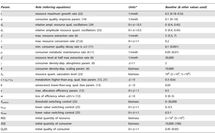
Param. Role (referring equations) Units* Baseline (& other values used)

r resource maximum growth rate (22) 1/mnth 0.5 (0.18–0.5))

a consumer quality response param. (14) 1/mnth 0.1 (0–10)

dr relative ampl. resource qual. oscillations (24) 0##,0.5 0 (0.4, 0.45)

ds relative amplitude resource quant. oscillations (23) 0###0.5 0 (0.4, 0.45)

d max. resource extraction rate (6) 1/mnth 5 (5.5, 7)

l max. resource conversion rate (21,6) 0###1 0.2

a min. consumer quality decay rate isa/d(11) # 0.1 (0.001)

m consumer metabolic maintenance rate (4,11) 1/mnth 0.05 (0.01)

b resource level at half max extraction rate (6) 1/mnth 30,000

c consumer density-dep. abruptness param. (6) #$1 2

K consumer density-dep. scaling param. (6) biomass 10,000

S0 resource quant. saturation level (23) biomass 106(26105, 56106)

c = cR= cX metabolism higher-than-avg. qual. bias param. (13, 21) #.0 0.3 (0.6)

b senescence lower-than-avg. qual. bias param. (13) #.0 0.05

v max. allocation efficiency param. (12) 0##,1 0.5

w loss of efficiency whenu(t)?_v(12) #.0 0 (0–5)

Xswitch threshold switching control (25) biomass 0–30,000

umin lower value switching control (25) 0###1 0–0.5

umax lower value switching control (25) 0###1 0.5-1

R(0) initial quantity of resource biomass 26105₍₅₆₁₀5₎

X(0) initial quantity of consumer biomass 10,000 (100)

QX(0) initial quality of consumer 0###1 0.45 (0.05)

*mnth = time in months, biomass units are arbitrary,

(7)

equation formulations we need to take care not to artificially induce oscillations of spurious period through an arbitrary choice of step size. Rather, step size should be selected to reflect generational processes, such as maternal effects, or seasonal processes (e.g. [61]) to reflect annual cycles in temperature and precipitation and the impacts these cycles have on the abundance and quality of biological resources that drive the dynamics of population exploiting these resources.

An interest in population fluctuations naturally leads to the question of the extent to which quantity-quality dynamics in-of-themselves induce oscillations in populations and what the periodicity of such oscillations would be. Since we know that seasonality can induce oscillations, as can consumer-resource interactions, we can only answer this question by separating out these various causes by considering the inherent ability of our quantity-quality formulation to induce oscillations in the absence of seasonal drivers and the coupling of populations to their resources at a lower trophic levels or their consumers at higher trophic levels. Thus we address the question in the specific context of oscillations in Eqs. 11–13 as a function of different parameter values, noting that the value of r, which we recall is given by

r=R/b(cf. Eq. 6 and 12), represents the underlying, but constant in this case, resource level that the population extracts for growth in the abundance measure x and average quality measure q. Furthermore, since this analysis necessarily assumes that all parameters are constant (i.e. seasonal drivers and other time-varying drivers are absent—such models are said to be autonomous), we assume u(t) is constant and, without loss of generality, selectu=vM_{(0,1). Further we note that the points 0 and} 1 are not included in this range sinceu= 0 impliesq(t)R2‘and

u= 1 implies x(t)R 2‘ as tR‘. In short, our focus is on the existence and stability of a finite equilibrium solutionðxx^,^qqÞto Eq. 11–13 for constantu.

In Appendix S2, we demonstrate that our Q-Q formulation does not produce oscillations when the background resources are fixed. This may seem a surprising result in light of the existence of well-described maternal effects leading to oscillations. However, in real populations background resources are never constant, unless very carefully controlled experimental approaches are taken to ensure such constancy. Thus, for example, colonies growing in Petri dishes or populations growing in well-mixed containers draw

down resources if the resources are not replenished through a constant resource input, such as in the experiment of [62]. The fact that our Q-Q model does not produce oscillations for populations embedded in a constant environmental (i.e. resource) background suggests that in real systems sustained oscillations arise either from through consumer-resource couplings, of which the Lotka-Volterra predation model [2,6] is the best known theoretical example, or through oscillatory forcing by underlying environ-mental drivers. In practice, of course, we typically see a complex combination of several consumer-resource interactions mutually intertwined through generalist feeding patterns and coupled with environmental forcing at several different frequencies (diurnal, lunar, seasonal, solar and earth’s orbit and spin-inclination cycles). It is worth reinforcing here that discrete-time equations cannot properly account for the effects that fluctuating environmental drivers have on demographic and ecological process if the cycles have periods less than size of the time step underpinning the equations. This statement applies equally if the quality of individuals is incorporated and that quality again exhibits changes in values over time scales smaller than the time step used to formulate the equation (e.g. if quality varies over seasons and the step size is annual, or if the quality varies across years and the step size is generational for organisms that live many years).

Differential equation formulations, by virtue of their continuity in time, avoid the pitfall arising from an inappropriate choice of model iteration step size, when addressing questions relating to the biological interpretation of characteristic oscillation frequencies associated with the model; although it behooves the analyst to ensure that the algorithms used to simulate the equations are numerically well-behaved (i.e. converge to the real solution as the simulation step-size decreases). In our simulations below, we first investigate how consumer abundance is impacted by the value of the allocation proportion parameter u(t) when assumed constant and set tovso that extraction function expressed in Eq. 12 is now independent ofuandvand reduces to

I(x)~ kdpk

pkzkzeyx ð16Þ

We then consider how this resource extraction allocation function, switching between growth in consumer abundance (u(t) = 0) and elevation of quality (u(t) = 1), can stabilize population fluctuations, including if the switching is incomplete: i.e. u(t) switches betweenuminandumax, where0vuminvumaxv1.

Consumer-Resource Interactions

To obtain new insights into factors influencing the period and amplitude of oscillating populations, we begin by extending the metaphysiological consumer-resource model, represented by Eqs. 7, to our Q-Q framework modeled by Eqs. 11–13. After that we explore the oscillatory behavior of a simplified version of this four-dimensional model under the assumption of seasonal drivers underlying resource abundance and quality.

In our metaphysiological Q-Q framework, denoting the actual (i.e. not logarithmic) abundance of the resource byRand that of the consumer byX, and their untransformed quality indices byQR and QX respectively, the interactions are described by the four equations (Table 1)

1

R dr

dt~urI(R){f(R,X)XzaRlnQR ð17Þ

Figure 1. Consumer equilibrium abundanceXX^(scale 1 = 30,000

biomass units) is plotted for the baseline set of parameters

(Table 2) as function of u (the proportion of extracted

resources extracted that are invested in increasing abundance

versus the proportion 1-u invested in increasing consumer

quality QX). Nonzero equilibrium abundance values only occur for

u$0.11, and a maximum equilibrium abundance of 28,638 biomass units occurs atu= 0.704.

(8)

1

QR

dQR

dt ~{aRlnQR(1{uR)IR(R)

{cRf(R,X)X{bRaRlnQR

ð18Þ

1

X dX

dt~uXkX(QR)f(R,X)R{mXzaXlnQX ð19Þ

1

QX

dQX

dt ~{aXlnQX(1{uX)kX(QR)f(R,X)R{

cXmX{bXaXlnQX

ð20Þ

whereI(R) expressed in Eq. 16 is the resource population’s per-capita extraction rate (Ris a photon or nutrient flux if the resource is a plant or is a plant population if the resource is a herbivore),

f(X,R) expressed in Eq. 6 is the consumer population’s per-capita per-unit resource feeding-rate function, andmXis the rate at which exploiters expend biomass to meet metabolic needs.

In our formulation of Eqs. 11–13, we mentioned that the conversion ratek_.0 should be a decreasing function of resource quality QR in the case of herbivory since, for example, lower quality plants are those that are either defended by chemical compounds that the consumer needs to detoxify or through inclusion of indigestible fiber in leaves and other grazed parts of the plant. A relatively simple function that accounts for the bias that extracted resources will have a higher-than-average quality than the resource population itself, and is dependent on the senescence rate bias parametercR.0, is

k(QR)~lQ 1=(1z_cR)

R ð21Þ

where 0,l,1. To verify that this form has the desired properties we note that: i.) for any cR.0 the resource quality has at its theoretical (i.e. not realized in practice) maximumk(1) =lwhen

QR= 1 and its theoretical minimumk(0) = 0 whenQR= 0; ii.) the function is linear inQRforcR= 0 (i.e. when there is no bias in the senescence rate as function of quality) and iii.) the function is

increasingly super-linear in cR—i.e. lQ

1=(1z_cR)

R wlQ

1=(1z_cR)

R for

any 0,QR,1 whenever c1.c2—so that the quality extracted is increasingly higher than average with increasingc.

Seasonal Drivers

As a first step to understanding the dynamics of a consumer exploiting a resource that varies seasonally in both abundance and quality, we simplify Eqs. 17 and 18 as follows. First, we assume the resource grows logistically, driven by a seasonally varying carrying capacityS(t)—i.e. in Eq. 17 we make the substitution

uRI(R){f(R,X)zaRlnQR

:r 1{ R

S(t)

[dR

dt~rR 1{ R S(t)

ð₂₂Þ

where, assuming the units of time are months, we set

S tð Þ~S0ð0:5zdSsin 2ð pt=12ÞÞ: ð23Þ

This latter form implies that the parameter 0#dR,0.5 determines the amplitude ofS(t).0 around its average valueS0. Second, we remove Eq. 18 for the quality of the resource and replace it with the periodic input function

QRð Þt ~0:5zdRsin 2ð pt=12Þ, ð24Þ

where 0#dR#0.5 ensures that 0#QX#1, and has an average value of 0.5.

In this case Eqs. 17–20 reduce to a system of three equations containing the following time constants, characterizing five key processes that influence the period and amplitude of oscillations when they emerge as a result of the consumer-resource interaction process:

1. A maximum resource per-capita growth rater: this rate occurs at densitiesR(t) well below the carrying capacity S(t), with a concomitant per-capita decline rate of negativerthat occurs at double the carrying capacity density (this can arise if the carrying capacityS(t) drops considerably through its seasonal cycle).

2. A maximum resource extraction rated: this rate is reduced by the resource quality variableQR(t), which we expect to average around 0.5 in our simulations, and is also reduced by a normalized functional response to resource and consumer densities F = f(R,X)R/d, which satisfies 0#F,1 (F is 1 when resources are large and consumers are not too large, and close to 0 when resources are low or consumer-to-resource density ratio is relatively large).

3. A maximum consumer rate of increaseld: (cf. Eq. 21) this rate isltimes the resource extraction rate and so is also modified by the current value ofF.

4. A maximum consumer rate of decay (m=m-alnQX): although this rate may typically be in the range [m,m+10a] (note: ln

QX,0), it can rise without bound if consumer quality plummets. In doing so, it will then rapidly drive the population to 0 as individuals become starved of resources.

5. A consumer quality response ratea: this rate scales the response of the consumer quality variable to changes in the resource extraction rate, but is moderated by how close the quality variable is to 1 with the rate of approach to 1 declining linearly with distance from 1. It also scales the rate of increase in quality due to preferential removal of low quality individuals during the decay process, with a scaling constantbdetermining the extent to which decay acts differentially on low quality individuals. Also together with a second scaling constant c, the parameteradetermines the maximum rate at which quality declines when at its maximum value ofQX= 1.

In our analysis we select a baseline set of population parameter values (Table 2) and then explore the impact of introducing seasonal drivers (by making parametersdSanddRin Eqs. 23 and 24 non-zero), changing the response-time constants of the resource (contrasting values of the parameter r) and consumer quality (contrasting values of the parameter a) equations, as well as perturbing the maximum value of the resource extraction rate (contrasting values of the parameter d). Most importantly, however, we also explore the effects of different investment rates

u in the relative proportion of resources that are allocated to increasing population abundance versus elevating the average quality of the population under the simplifying assumption that

u(t) =v, where as discussed earlier (cf. Eq. 12)vis assumed to be the most physiologically efficient value ofuover the long term. In a final simulation, we explore aspects of allowingu(t) to respond to seasonal changes in population abundance.

(9)

resource qualityQR(t). For generality and simplicity, we will not specify the units of biomass other than to assume the units ofX(t) andR(t) are in the same units, noting that the parametersKandS0 scale the equilibrium levels of the consumer and resource populations respectively in these same units. All rate parameters are in units of inverse months (1/mnth) so that if a rate parameter has a value of 0.5, then after 1 month it will have caused the population to increase to approximately e0.5

= 1.65 (165%) or decrease to approximately e20.5

= 0.61 (61%). Conversely, if an individual consumes 5% of its body weight per day, which is 150% of its body weight per month, then the per-capita instantaneous rate of resource consumption is ln(1.5) = 0.41. The doubling (parameters associated with increases) or halving (parameters associated with decreases) time of any of our variables under the influence of a parameterpis calculated using the equationt= ln2/

p, which is a convenient way to characterize the response time of a rate parameter.

Numerical simulation of Eqs. 19–24, using the baseline set of parameter values, reveal that in a constant resource environment (i.e. dR= 0.0 anddS= 0.0) population abundance equilibrates for all constant values of the extraction rate allocation proportionu

within the range [0,1] (Fig. 1; a typical trajectory is given in Fig. 2A). The equilibrium values XX^u so obtained, however, are

only non-zero (in effect exceed the cutoff threshold of 1) for

u.0.11, achieving a maximum value ofXX^u~28,638atu= 0.704.

As we previously mentioned, this is the value obtained by substituting the model parameter values in the expression given by Eq. 15, even though this equation was derived for the two-dimensional system modeled by Eqs. 11–13, while the values in Fig. 1 are derived from numerically simulating the long-term behavior of the higher dimensional model represented by Eqs. 19– 24. The reason for the equivalence is that the optimal investment

proportion given by Eq. 15 does not depend on parameters in the extraction function Eq. 12, so that in the absence of seasonal drivers in Eq. 22–24 (i.e.dR= 0.0 and dS= 0.0) the equilibrium consumer abundance levels in both systems, though different because the resource levels supporting the consumers in the two models are different, will be maximized by the same valuev*+

whenever the remaining parametersa,b, c,aandmare the same in both models. Again we stress, because the issue of verification is so central to the confidence we can place in our numerical results, that the agreement of values computed in two completely independent ways provides mutual co-verification for the math-ematical correctness of our analytical expressions and for the computer code used to generate our numerical results.

The approach of both the resource and consumer solutions to equilibrium values (Fig. 2A), used to produce Fig. 1, is lost once environmental forcing is included in the resource equations. We now consider the impact of seasonal forcing on the abundance of the consumer and its feedback on the oscillating resources. First we consider the case when only the quality of the resource oscillates over a 9-fold range of values (Fig. 2B.dR= 0.45,dS= 0.0). In this case the behavior is rather regular with the seasonal forcing of resource quality producing relatively small oscillations on the abundance of the consumer that then feedback to produce even smaller oscillations on the abundance of the resource. When the resource abundance itself is made to oscillate over a 9-fold range around its baseline value while resource quality is kept at its baseline value, then the abundance of the consumer begins to show strong oscillations that are amplified through feedback with a significant drop in the average consumer and resource values over the 25-year (300-month) simulation interval (Fig. 2C. dR= 0.0,

dS= 0.45). The frequency of these oscillations is approximately 1/5 per year (implying a period of 5 years). If a 9-fold resource quality oscillation is now imposed on top of the 9-fold resource abundance oscillations, the 1/5 frequency and large amplitude of the consumer oscillations dominate, but now with a small amplitude wave of frequency 1—i.e. the annual frequency of the resource quality oscillations—imprinted upon it (Fig. 2D dR= 0.45,

dS= 0.45).

The size of the oscillations, the shape of the transients, and even the frequency of the dominant oscillations appearing in Fig. 2 are rather sensitive to the different relative values of the time constants associated with the five key processes listed above (Fig. 2E–F). For example, in the absence of seasonal forcing when the maximum extraction ratedis increased from 5 to 5.5, the equilibrium is lost and a cycle of period 8-years emerges (Fig. 2E,d= 5.5,dR= 0.0,

dS= 0.0). Interestingly, if seasonal forcing is now reintroduced (Fig. 2F,d= 5.5,dR= 0.45,dS= 0.45) the period 8 oscillations are lost and the period 5 oscillations return, indicating how the emergent oscillations have periods that are nonlinearly dependent on underlying population process rates and seasonal drivers.

Periods and Relative Rates

By changing the relative values of the different rate constants listed above, all kinds of behavior can be induced in the abundance of consumers, from extinction, through the existence of a positive stable equilibrium, to stable oscillations with a range of periods. As observed, though, by Murdoch et al. [63] and elucidated by Ginzburg and Colyvan [15], consumers specializing on a single resource are unlikely to oscillate with periods less than 6, unless driven by seasonal drivers, in which case the oscillations may collapse to period 1, the period of the seasonal cycle. Our model exhibits this same behavior (Table 3), as we vary the resource response rate parameter r and the consumer quality response rate parametera, with the remaining parameters at their

Figure 2. Consumer abundance X(t) (black: scale 1 = 40,000

biomass units) and resource abundance R(t) (red: scale

1 = 500,000 units) are plotted over 300 months for the set of baseline parameters listed in Table 1 for the cases of periodic

environmental forcing: A.no forcing (dR= 0.0,dS= 0.0);B.resource

quality forcing (dR= 0.45,dS= 0.0);C.resource abundance forcingS(t)

(dR= 0.0, dS= 0.45); D. resource quality and abundance forcing

(dR= 0.45,dS= 0.45);E.parameters as in A. exceptdhas been increased

from 5 to 5.5;F.parameters as in E. except seasonal forcing (dR= 0.45, dS= 0.45) has been added.

(10)

baseline values (Table 2) in both constant (dR= 0.0, dS= 0.0) and seasonally forced (dR= 0.45, dS= 0.45) backgrounds. In the constant background, the consumer-resource interaction supports a stable equilibrium (Fig. 2A) for the baseline parameters, but as the resource response rate decreases (Table 3A, Case 1) from

r= 0.5 in steps of 0.01, oscillations set in atr= 0.48 with the rather long period of approximately 18 years. This drops to a minimum period of around 8 years forraround 0.40 to 0.35 and starts to increase up to a period of approximately 12 years atr= 0.21. For

r#2.0 the consumer population goes extinct. If seasonal forcing is added (Table 3A, Case 2) then the period is smallest at just under 5 years for the fastest resource response rate considered (r= 0.5) rising to around 11 years atr= 0.19, but going extinct forr#0.18. The question of how the periods of oscillations arising from consumer-resource interactions are influenced by various rate constants in the model can certainly be addressed using current Lotka-Volterra-like and other first-order species model paradigms, including discrete-time paradigms; e.g. as discussed by Murdoch et al. [7]. However, the question of how the average quality of a

population will impact such oscillations cannot even be asked using these approaches, but requires a Q-Q paradigm of the type formulated here. We addressed this question using Eqs. 19–24 (Table 3B). Our analysis indicates that when the quality response rate to resource intake is 0, the population goes extinct because quality asymptotically approaches 0. For non-zero quality response ratesa.0, relatively small (i.e. slow) response times have little effect and abundance oscillates with its seasonal drivers—i.e. the period is 1. As the quality variable comes into play with increasing responses timesa, so the period begins to increase. For the caser= 0.5 (Table 3B, Case 1) the period jumps from 1 to 4.3 ata= 0.06 and then increase steadily to cap out at around 8 years. For the caser= 0.3 (Table 3B, Case 2) the period jumps from 1 to 5.6 ata= 0.03 and then steadily increases to cap out at around 10 years, though unlike the caser= 0.5 the consumer goes extinct for

a$0.77 (not shown).

Allocation Switching and Stabilization

The fact that quality has an influence on the period of oscillations that arise from consumer-resource interactions raises the question of the extent to which individuals can dampen or alter the period of consumer-resource oscillations by manipulating the proportion of resources over time that they allocate to growth in abundance versus elevating the average quality in the population. The most extreme version of this type of manipulation is to switch back and forth betweenu(t) = 0 (all extracted resources allocated to elevating the average quality of individuals in the population) and

u(t) = 1 (all extracted resources allocated to increasing population abundance). In the context of maximizingJ defined in Eq. 14, solutions that switch between lower and upper bounds are called ‘‘bang-bang’’ and are known to be optimal when the problem is linear in the ‘‘control’’ function u(t), though so-called singular control components, whereu(t) =v and v is a constant that lies between 0 and 1, also play a role in the optimal solution over a central segment of the interval [0,T] [56].

For systems that are not fully described by the equations used to model their dynamics (in our case Eqs 17–20 are only an approximate description of the processes driving change in the variables of interest) and for systems that are subject to stochastic perturbations, an ‘‘open-loop solution’’ to a formulated determin-istic maximization problem, as in encapsulated in our Eq. 14, is moot. More appropriate are ‘‘feedback or adaptive solutions’’ that self-correct when the model strays from reality: such solutions posit explicit explanations of how organisms have evolved to respond to change that is not completely predictable [64]. Thus rather than solve for the optimal solution that corresponds to our specific set of baseline parameters (which themselves are of no special signifi-cance), we explore how feedback rules based on the state of the variables perform in stabilizing population fluctuations. As recently hypothesized and demonstrated by Ginzburg et al. (in review) in the context of discrete time models, populations appear to have evolved to avoid the large fluctuations, because populations are most vulnerable to extinction every time they pass through a trough of a large amplitude oscillation.

The first feedback rule we investigate, motivated by the structure of optimal solutions to Eq. 14, is to select a critical abundance levelXswitchand define:

u~uminwheneverX tð ÞƒXswitchelseu~umax: ð25Þ

IfXswitchis too large then control is always at its maximum value; as in the case of the baseline values, exceptd= 7, under seasonal forcing (dR= 0.45, dS= 0.45) with umin= 0 and umin= 1 and

Xswitch.29,300 (Fig. 3A). As Xswitch is reduced for the baseline

Table 3.Period of consumer-resource oscillations for selected values of the resource response rater(A.) and the consumer quality response ratea(B.), with the remaining parameters at their baseline values (Table 2) except as noted.

Parameter Case 1 Case 2

A.:r No seasonality

dR= 0 anddS= 0

Seasonal Forcing

dR= 0.45 anddS= 0.45

0.5* Equilibrium Period,4.8

0.49 Equilibrium Period,4.9

0.48 Period,18 Period,4.9

0.21 Period,12 Period,10

0.20 Extinction Period,10

0.19 Extinction Period,11

0.18 Extinction Extinction

B.:a Baseline responser= 0.5

dR= 0.45 anddS= 0.45

Rapid responser= 0.3

dR= 0.45 anddS= 0.45

0.00 Extinction Extinction

0.02 Period 1 Period 1

0.03 Period 1 Period,5.6

0.05 Period 1 Period,6.3

0.06 Period,4.3 Period,6.7

1.00 Period,6.8 Extinction

10.0 Period,7.2 Extinction

(11)

set of parameters, control increasingly clips the peaks of the oscillations (Figs. 3B and 3C), thereby reducing the troughs until the consumer population becomes relatively steady around

Xswitch= 4,000 (Fig. 3D). The control, however, chatters on-and-off at relatively high frequencies for most of the year, but this can be reduced to chattering for only part of the year if the allocation switching is not complete, but set to umin= 0.1 and umin= 0.9 (Fig. 3E). If the allocation range is further reduced to toumin= 0.3 andumax= 0.7 (Fig. 3F), then switching only occurs once toumax and once toumineach year, but the oscillations in the consumer population again become relatively large.

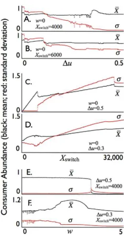
Graphs of the mean and standard deviation of fluctuations in consumer population abundance over a 20-year interval (Fig. 4: years 80–100 are selected from the simulations to avoid transients peculiar to the initial conditions) are plotted over ranges of values for the allocation parameter u (Figs. 4A–B), for the threshold parameterXswitch(Figs. 4C–D), and the loss of efficiencywin the deviation of the allocation u from the optimal value v= 0.70 (rounded to 2 d.p.) (Figs. 4E–F). As the range Du= umax- umin increases (cf. Eq. 25), the mean population level XX remains relatively constant while the standard deviation s steadily decreases over most of the range (Figs. 4A–B), although small regions do exhibit somewhat irregular behavior due to the highly nonlinear nature of the model. Also in the caseXswitch= 4,000, a favorable region does occur around Du= 0.35 where the abundance is about 20% higher than for most other values ofu

and the standard deviation takes a noticeable drop down to close to zero forDu$0.35 showing the allocation switching rule Eq. 25 is very effective at stabilizing the otherwise strongly oscillatory consumer-resource interaction (cf. Fig. 3A versus 3D).

If Xswitch is too large though, e.g. Xswitch= 6,000, then stabilization is only partial and the standard deviationsremains relatively high over forDuat its most extreme (i.e. over the range 0.4 to 0.5). This is amply demonstrated in Figs. 4C–D where we see that althoughXX increases withXswitchthe standard deviations increases much faster once Xswitch gets beyond 4,900, at which point allocation switching looses its ability to completely dampen the oscillations (note, in Fig. 4C, thats is almost zero and then takes a jump around Xswitch= 4,900). The graph in Fig. 4C.

indicates a clear advantage for the combinationXswitch= 4,900 and

Du$0.5 in maximizing the average abundance while completing dampening the oscillations for the baseline set of parameters (though withd= 7 rather than 5).

The graphs in which we vary the efficiency parameter w

(Figs. 4E–F) indicate that a switching allocation strategy remains very effective even when there is a costw.0 to deviating from the physiologically optimal allocation point ofv= 0.7 for our baseline parameters (Fig. 1). The stabilization remains relatively insensitive tow for the case of extreme switching (Fig. 4E Du= 0.5) (with mean abundance decreasing only slightly and the standard deviation in this abundance increasing only slightly) until whits a threshold at w= 3.4, beyond which the consumer population collapses because it cannot bear the level of cost associated with inefficiencies deviating from the physiologically optimal allocation point v= 0.7. Some unexpected happens, however, for the case

Du= 0.3 (Fig. 4F). In this case consumer abundance is maximized, with a corresponding relatively low associated standard deviation, when the population efficiency parameter has the nonzero value

w= 2.46, implying, as we discuss further below, that some cost to allocation switching is beneficial to the population as a whole.

Allocation Modes and Growth Patterns

Seasonal growth patterns in which organisms allocate resources to different organ systems—e.g. vegetative structures roots and tubers, or reproductive structures—are well known in plants and animals [65,66]. The type of tissue laid down in these different organ systems can be viewed as representing different intrinsic quality levels with switches from one growth mode to another subject to resource-demand versus extracted-supply related physiological signals [18]. This sort of growth mode switch does not necessarily require external seasonal signals, but may be linked to signals generated intrinsically through stresses brought about by crowding; with this phenomenon being evident across the organismal spectrum including bacteria, protists, fungi, plants, invertebrates and vertebrates.

Recently [27] presented their deconstruction of what they refer to as a typical growth curve of lab-cultured microbial populations. They identify five to six phases that include (cf. Fig. 1 in [27]): 1.)

Figure 3. The trajectories of consumer abundanceX(t) (black: scale 1 = 30,000 units) and qualityQX (red: scale 0–1), resource

abundanceR(green: scale 1 = 600,000) units) and resource extraction allocation functionu(t) (blue: scale 0–1) given by Eq. 25 are

plotted over years 80–100 (to avoid effects of initial conditions) of a simulation driven by strong season fluctuations in resource

carrying capacity and quality (dR= 0.45,dS= 0.45) for the baseline parameters, except hered= 7 andXswitchvaries in steps of 100, for

the following cases, with statistics forX(t) (min, max, mean, square-root of variance) calculated over years 80–100 in parenthesis: A.

umin= 0, umax= 1, Xswitch= 29,300 (Xmin= 410, Xmax= 29292, XX= 5486, s= 7541); B. umin= 0, umax= 1, Xswitch= 15,000 (Xmin= 295, Xmax= 15054,

X

X= 5035,s= 4990);C.umin= 0,umax= 1,Xswitch= 7,000 (Xmin= 384,Xmax= 7049,XX= 3881,s= 2520);D.umin= 0,umax= 1,Xswitch= 4,000 (Xmin= 3997,

Xmax= 4038, XX= 4009, s= 11); E. umin= 0.1, umax= 0.9, Xswitch= 4,000 (Xmin= 3998, Xmax= 4578, XX= 4225, s= 214); F. umin= 0.3, umax= 0.7, Xswitch= 4,000 (Xmin= 614,Xmax= 9655,_X_X_{= 4076,}_s_{= 2719).}

(12)

an initial lag phase in which the culture takes a characteristic ‘‘lag time’’ to begin growing; 2.) a stronger than exponential phase of growth (which they call the logarithmic exponential or LogEx phase); 3.) an exponential phase (which they call the regular exponential or RegEx phase); 4.) an inhibition phase; 5.) a stationary phase; and possibly 6.) a decay/decline phase. They analyze several different classes of models that have been developed to capture all these different phases and they conclude that since ‘‘all the theoretical and numerical results presented for delay growth models are contrary to the experimental evidence regarding the conditions for the occurrence of a lag phase, we may conclude that delay effects and the lag are two distinct biological phenomena.’’ The implication of this is that the lag phenomenon cannot simply be captured through the inclusion of time delays in existing growth models but require an additional dimension to the analysis, such the inclusion of a quality dimension.

These six phases can be captured easily through the allocation switching logic provided by Eq. 25. In Fig. 5 we illustrate these phases for the case umin= 0.07, umax= 0.85 and Xswitch = 1000.

Thus, if the quality and abundance are initially low at the start of a microbial culturing experiment, the population focuses on increasing its quality, thereby producing a lag phase in its growth in abundance until the abundance variable crosses a threshold. Rapid growth is then experienced (LogEx phase), followed by steady growth (RegEx phase), followed by inhibition and then stationarity as density dependence sets in. Note that we could have fashioned the trajectory in Fig. 5 to closely resemble the growth curve idealized in Fig. 1 of [27] by making the allocation switch occur over a finite period of time rather than instantaneously, thereby removing the sharp corner in the abundance trajectory at the switch. The purpose of Fig. 5, however, is merely to demonstrate how allocation switching, whether sharp or gradual, can produce a variety of empirical growth patterns that have been observed in nature or laboratory cultures. One can imagine even more complex growth patterns if switching is based on thresholds in both the quality and abundance rather than just the abundance alone. Finally, due to a decline in quality over the stationary phase, a sample from the population depicted in Fig. 5, if now moved to another culture dish as was done in the experiments described in [27], will exhibit the same pattern of growth because, in the new dish, the initial conditions are now once again low quality and low abundance.

Discussion

Theoretical population ecology during most of the 20thCentury has been developed around an abundance (i.e. quantity) variable involving numbers of individuals, or number or biomass densities. Additionally, populations have been structured into age, size or life-history stage classes ([67,68,69]; also see [7,18,37,70]). This is not to say that other subfields of ecology such as physiological and ecosystem ecology have not used other currencies (energy, kinds of molecules, nutrient classes) to discuss individual or community level dynamic processes [71,72]. In consumer-resource or food web abundance (biomass/numbers-density) dynamics, however, the importance of a second-order description when trying to explain the source of oscillations that are observed in such systems has been largely neglected (to whit see [8]), with the exception being the work of Ginzburg and collaborators [15,19] and some efforts to include storage as an explicit process [32].

Figure 4. Consumer mean biomass density XX (black: scale

1 = 6,000 units) and its standard deviation s (red: scale

1 = 6,000 units) averaged over a 1000 year period for the

allocation parameter u switching between umin= 0.5-Du

(X#Xswitch) and umin= 0.5+Du (X.Xswitch) with the conversion

deviation efficiency cost parameter w allowed to vary as

indicated.The rest of the parameters are baseline values (Table 2)

except thatd= 7,dR= 0.45 anddS= 0.45, with values forXswitch,Du, and w:A. & B.Duranging from 0 to 0.5 in steps of 0.001,v= 0.5;C. & D. Xswitchranging from 0 to 32000, in steps of 50;E. & F.wranging from 0 to 5 in steps of 0.01 (cf. individual trajectories used to obtain the mean and standard deviation for selected values ofDuandXswitchin Fig. 3, but averaged here over 1000 years to minimize the impact of the initial conditions).

doi:10.1371/journal.pone.0014539.g004

Figure 5. The trajectories of population (consumer) abundance

X(t) (black: scale 1 = 30,000 units; X(0) = 100) and quality QX

(red: scale 0–1; QX(0) = 0.05), and the resource extraction

allocation function u(t) (green: scale 0–1) satisfying Eq. 25,

withumin= 0.07,umax= 0.85 andXswitch = 1000 are plotted over

600 units of time (no longer interpreted as months) under the

constant resource conditionsR(t) = 500,000 (instead of Eqs. 17

and 22) andQR(t) = 0.5 fortM[0,500], for the remaining baseline

parameters as in Table 1 with the exceptions that here

a= 0.001,m= 0.01,c= 0.6,w= 1.