Influence of meteorology and interrelationship with greenhouse gases (CO<sub>2</sub> and CH<sub>4</sub>) at a sub-urban site of India

(1)

ACPD

15, 34205–34241, 2015

Influence of meteorology on GHGs and their interrelationship

G. Sreenivas et al.

Title Page

Abstract Introduction

Conclusions References

Tables Figures

◭ ◮

Back Close

Full Screen / Esc

Printer-friendly Version Interactive Discussion

Discussion

P

a

per

|

Discussion

P

a

per

|

Discussion

P

a

per

|

Discussion

P

a

per

|

Atmos. Chem. Phys. Discuss., 15, 34205–34241, 2015 www.atmos-chem-phys-discuss.net/15/34205/2015/ doi:10.5194/acpd-15-34205-2015

This discussion paper is/has been under review for the journal Atmospheric Chemistry and Physics (ACP). Please refer to the corresponding final paper in ACP if available.

Influence of meteorology and

interrelationship with greenhouse gases

(CO

₂

and CH

₄

) at a sub-urban site of India

G. Sreenivas, P. Mahesh, J. Subin, A. L. Kanchana, P. V. N. Rao, and V. K. Dadhwal

Atmospheric and Climate Sciences Group (ACSG), Earth and ClimateScience Area (ECSA), National Remote Sensing Center (NRSC), Indian Space Research Organization (ISRO), Hyderabad, 500037, India

Received: 28 October 2015 – Accepted: 21 November 2015 – Published: 4 December 2015

Correspondence to: P. Mahesh (mahi952@gmail.com)

Published by Copernicus Publications on behalf of the European Geosciences Union.

(2)

ACPD

15, 34205–34241, 2015

G. Sreenivas et al.

Title Page

Tables Figures

◭ ◮

Back Close

Full Screen / Esc

Discussion

P

a

per

|

Discussion

P

a

per

|

Discussion

P

a

per

|

Discussion

P

a

per

|

Abstract

Atmospheric greenhouse gases (GHGs) such as carbon dioxide (CO2) and methane

(CH4) are important climate forcing agents due to their significant impact on the climate

system. The present study brings out first continuous measurements of atmospheric GHG’s using high precision Los Gatos Research’s-greenhouse gas analyser

(LGR-5

GGA) over Shadnagar, a suburban site of Central India during the period 2014. The annual mean of CO₂ and CH₄ over the study region is found to be 394±2.92 and 1.92±0.07 ppm (mean, µ±1 SD, σ) respectively. CO2 and CH4 showed a significant

seasonal variation during the study period with maximum (minimum) CO2 observed

during Pre-monsoon (Monsoon), while CH₄recorded maximum during post-monsoon

10

and minimum in monsoon. A consistent diurnal mixing ratio of these gases is observed with high (low) during night (afternoon) hours throughout the study period. Influences of prevailing meteorology (air temperature, wind speed, wind direction and relative hu-midity) on GHG’s have also been investigated. CO2and CH4showed a strong positive

correlation during winter, pre-monsoon, monsoon and post-monsoon withR equal to

15

0.80, 0.80, 0.61 and 0.72 respectively. It implies the seasonal variations in source-sink mechanisms of CO2and CH4. Present study also confirms implicitly the presence OH

radicals as a major sink of CH4over the study region.

1 Introduction

The Intergovernmental Panel on Climate Change (IPCC, 2013) reported that

hu-20

mankind is causing globalwarming through the emission of greenhouse gases (GHG),particularly carbon dioxide (CO₂) and methane (CH₄). CO₂ and CH₄ concen-trations have increased by 40 and 150 % respectively since pre-industrial times, mainly from fossil fuel emissionsand secondarily from net land use change emissions (IPCC, 2013). CO₂measurements at Mauna Loa, Hawaii (Monastersky, 2013) have exceeded

25

(3)

ACPD

15, 34205–34241, 2015

G. Sreenivas et al.

Title Page

Tables Figures

◭ ◮

Back Close

Full Screen / Esc

Discussion

P

a

per

|

Discussion

P

a

per

|

Discussion

P

a

per

|

Discussion

P

a

per

|

due to high uncertainty in its sources and sinks (Keppler et al., 2006; Miller et al., 2007; Frankenberg et al., 2008). Kirschke et al. (2013) reported that in India, agriculture and waste constitutes the single largest regional source of CH4. Although many sources

and sinks have been identified for CH₄, their relative contribution to atmospheric CH₄ is still uncertain (Garg et al., 2001; Kirschke et al., 2013). In India, electric power

gen-5

eration that contributes to half of India’s total CO2 equivalent emissions (Garg et al.,

2001).

Global climate change has serious impact on humans andecosystems. Due to this, many factors have been identified that may reflector cause variations in environmental change (Pielke et al., 2002). Out of these, the Normalized Difference Vegetation Index

10

(NDVI) has become one of the most widely used indices to represent the biosphere influence on global change (Yang et al., 2011). The planetary boundary layer (PBL) is the part of the atmosphere closest to the Earth’s surface where turbulent processes often dominatethe vertical redistribution of sensible heat, moisture, momentum, and aerosols/pollution (Ao et al., 2012).

15

Greenhouse and other trace gases have great importance in atmospheric chemistry and for radiation budget of the atmosphere–biosphere system (Crutzen et al., 1991). Hydroxyl radicals (O ˙H) are very reactive oxidizing agents, which are responsible for the oxidation of almost all gases that are emitted by natural and anthropogenic activi-ties in the atmosphere. Atmospheric CO₂measurements are very important for

under-20

standing the carbon cycle because CO2 mixing ratios in the atmosphere are strongly

affected by photosynthesis, respiration, oxidation of organic matter, biomass and fossil fuel burning, and air–sea exchange process (Machida et al., 2003).

The present study brings out first continuous measurements of atmospheric GHG’s using high precision Los Gatos Research’s-greenhouse gas analyser (LGR-GGA) over

25

Shadnagar, a suburban site of Central India during the period 2014. In addition to GHG’s observations, we have also made use of an automatic weather station (AWS) data along with model/satellite retrieved observation during the study period. Details about study area and data sets are described in the following sections.

(4)

ACPD

15, 34205–34241, 2015

G. Sreenivas et al.

Title Page

Tables Figures

◭ ◮

Back Close

Full Screen / Esc

Discussion

P

a

per

|

Discussion

P

a

per

|

Discussion

P

a

per

|

Discussion

P

a

per

|

2 Study area

Shadnagar is situated in Mahabubnagar district of newly formed Indian state of Telan-gana. It is a rural location situated∼70 km away from urban site of Hyderabad (North-ern side) with a population of ∼0.158 million (Patil et al., 2013). A schematic map of study area is shown in Fig. 1a. Major source of pollutants over Shadnagar can be

5

from small and medium scale industries, biomass burning and bio-fuel aswell as from domestic cooking. In the present study sampling of GHG’s and related meteorolog-ical parameters are carried out in the premises of National Remote Sensing Center (NRSC), Shadnagar Campus (17◦02′ N, 78◦11′ E). Sampling site is near to National highway 7 (NH7) and a railway track (non-electrified) is in the East (E) direction.

10

Mean monthly variations of temperature (◦C) and RH (%) observed at Shadnagar during 2014 are shown in Fig. 1b and c respectively. The Indian Meteorological Depart-ment (IMD) defined monsoon as June–July–August–September (JJAS), post-monsoon (October–November–December – OND), winter (January–February – JF) and pre-monsoon (March–April–May – MAM) in India. Temperature over Shadnagar varies from

15

∼20 to∼29◦C. Relative humidity (RH) in Shadnagar reached a maximum of 82 % in monsoon from a minimum of 48 % recorded during pre-monsoon. Surface wind speed (Fig. 1d) varies between 1.3 to 1.6 m s−1 with a maximum observed during monsoon and minimum in pre-monsoon. The air mass advecting (Fig. 1e) towards study site is either easterly or westerly. The easterly wind prevails during winter and gradually shifts

20

to south-westerlies in pre-monsoon, and dominates during monsoon.

3 Data set and methodology

Details about the instrument and data utilized are discussed in this section. The avail-ability and frequency of the observations all data used in present study are tabulated in Table 1.

(5)

ACPD

15, 34205–34241, 2015

G. Sreenivas et al.

Title Page

Tables Figures

◭ ◮

Back Close

Full Screen / Esc

Discussion

P

a

per

|

Discussion

P

a

per

|

Discussion

P

a

per

|

Discussion

P

a

per

|

3.1 In-situ observations

3.1.1 Greenhouse Gas Analyser (GGA)

The Greenhouse Gas Analyser (model: LGR-GGA-24EP) is an advanced instrument capable of simultaneous measurements of CO2, CH4 and H2O. This instrument is

well known for high precision and accuracy which are crucial towards understanding

5

background concentrations of atmospheric GHGs, with specifications meeting WMO standards of measurement. It is based on enhanced Off-Axis Integrated Cavity Out-put Spectroscopy (OA-ICOS) technology (Paul et al., 2001; Baer et al., 2002), which utilizes true wavelength scanning to record fully resolved absorption line shapes. Con-sidering the rural nature of the site, flow rateis fixed to be 7 liters per minute (L m−1).

10

Ambient air entering the GGA is analysed using two near infrared (NIR) distributed feedback tunable diode lasers (TDL), one for a CO₂ absorption line near 1.60 µm (ν0=6250 cm

−1

) and the other to probe CH4 and H2O absorption lines near 1.65 µm

(ν0=6060.60 cm −1

). The concentration of the gases is determined by the absorption of their respective characteristic absorption lines with a high sampling time of 1 s. A

de-15

tailed explanation regarding the configuration, working and calibration procedure per-formed for GGA in NRSC can be found elsewhere in Mahesh et al. (2015). In the present study we used GGA retrieved CO₂ and CH₄ data. High resolution data are diurnally averaged and is used in further analysis. Due to failure of internal central pro-cessing unit (CPU) of the analyzer data is not recorded from pre-monsoon month of

20

May to a few days in June during the study period.

3.1.2 O3and NOx analyzer

Surface concentrations of O3and NOxhave been measured continuously using on-line analyzers Model No.s: 49i and 42i for O3and NOxrespectively, procured from Thermo Scientific, USA) since July 2014. The ozone analyzer is based on Beer–Lambert–

25

Baugher law which relates absorption of light to the concentration of species as its

(6)

ACPD

15, 34205–34241, 2015

G. Sreenivas et al.

Title Page

Tables Figures

◭ ◮

Back Close

Full Screen / Esc

Discussion

P

a

per

|

Discussion

P

a

per

|

Discussion

P

a

per

|

Discussion

P

a

per

|

operating principle and has an in-built calibration unit for conducting periodical span and zero checks. The NOx analyzer utilizes a molybdenumconverter to convert NO2

into NO and estimates the NO_x concentration by the intensity of light emitted during the chemiluminescent reaction of NO with O₃present in the ambient air. The analyzer is integrated with zero and span calibration which are performed twice monthly.

5

Simultaneous observations of meteorological parameters are obtained from an au-tomatic weather stations (AWS) located in the same campus.

3.2 Satellite and model observations

3.2.1 MODIS

Moderate-resolution Imaging Spectrometer (MODIS) is launched in December 1999

10

on the polar-orbiting NASA-EOS Terra platform (Salomonson et al., 1989; King et al., 1992). It has 36 spectral channels and acquires data in 3 spatial resolutions of 250, 500 m, and 1 km (channels 8–36), covering the visible, near-infrared, short-wave infrared, and thermal-infrared bands. In the present study we used monthly Nor-malised Difference Vegetation Index (NDVI) data obtained from Terra/MODIS at 5 km

15

spatial resolution. The NDVI value is defined as following ratio of albedos (α) at different wavelengths:

NDVI=α_α0.86µm+α0.67µm 0.86µm−α0.67µm

(1)

NDVI values can range from−1.0 to 1.0 but typical ranges are from 0.1 to 0.7, with higher values associated with greater density and greenness of plant canopies. More

20

(7)

ACPD

15, 34205–34241, 2015

G. Sreenivas et al.

Title Page

Tables Figures

◭ ◮

Back Close

Full Screen / Esc

Discussion

P

a

per

|

Discussion

P

a

per

|

Discussion

P

a

per

|

Discussion

P

a

per

|

3.2.2 COSMIS-RO

COSMIC (Constellation Observation System for Meteorology, Ionosphere and Cli-mate) is a GPS (Global Positioning System) radio occultation (RO) observation sys-tem (Wang et al., 2013). It consists of six identical microsatellites, and was launched successfully on 14 April 2006. GPS radio occultation observation has the advantage

5

of near-global coverage, all-weather capability, high vertical resolution, high accuracy and self-calibration (Yunck et al., 2000). Geophysical parameters like temperature and humidity profiles have been simultaneously obtained from refractivity data using one-dimensional variational (1DVAR) analysis. Further COSMIC-RO profiles are used to estimate planetary boundary layer height (BLH). BLH is defined to be the height at

10

which the vertical gradient of the refractivity or water vapor partial pressure is minimum (Ao et al., 2012), explained detail methodology for calculating the BLH from refractivity (N).

3.2.3 Hysplit model

The general air mass pathway reaching over Shadnagar is analysed using

HYS-15

PLIT model (Draxler and Rolph, 2003) (http://www.arl.noaa.gov/ready/hysplit4.html). We computed 5 day isentropic model backward air mass trajectory for all study days with each trajectory starting at 06:00 UTC and reaching study site, (Shadnagar) at dif-ferent altitudes(1, 2, 3 and 4 km). Even though the trajectory analysis have inherent uncertainties (Stohl, 1998), they are quite useful in determining long range circulation.

20

4 Results and discussion

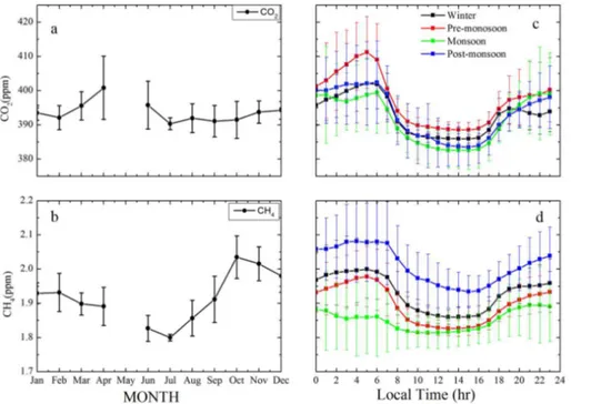
4.1 Seasonal variations of CO2and CH4

Monthly variations of CO2 and CH4 during the study period are shown in Fig. 2a and

b. Annual mean of CO2 over study region is found to be 394±2.92 (µ±1σ) ppm with

(8)

ACPD

15, 34205–34241, 2015

G. Sreenivas et al.

Title Page

Tables Figures

◭ ◮

Back Close

Full Screen / Esc

Discussion

P

a

per

|

Discussion

P

a

per

|

Discussion

P

a

per

|

Discussion

P

a

per

|

an observed minimum in monsoon and maximum in pre-monsoon. Background (av-erage) values of CO2 observed during different seasons are 393±5.60, 398±7.60,

and 392±7.0 and 393±7.0 ppm with respectively winter, pre-monsoon, monsoon and post-monsoon. Minimum CO₂ during winter (dry season) indicates the loss of carbon (Gilmanov et al., 2004) as decreased temperature and solar radiation during this

pe-5

riod inhibit increases in local CO2 assimilation (Thum et al., 2009). Enhancement in

Pre-monsoon is due to higher temperature and solar radiation prevailing during these months which stimulate the assimilation of CO2 in the daytime and respiration in the

night (Fang et al., 2014). Surface CO2concentration recorded a minimum during

mon-soon months can be mainly because of enhanced photosynthesis processes with the

10

availability of greater soil moisture (Patil et al., 2013). Further increase during post-monsoon CO2 is associated with high ecosystem productivity (Sharma et al., 2014)

also an enhancement in soil microbial activity (Kirschke et al., 2013).

CH₄ concentration in the troposphere is principally determined by a balance be-tween surface emission and destruction by hydroxyl radicals (O ˙H). The major sources

15

for CH4 in the Indian region are rice, paddies, wetlands and ruminants

(Schneis-ing et al., 2009). Annual CH₄ concentration over study area is observed to be 1.92±0.07 ppm, with a maximum (2.02±0.01 ppm) observed in post-monsoon and minimum (1.85±0.03 ppm) in monsoon. The highest concentration appears during post-monsoon and may be associated with the Kharif season (Goroshi et al., 2011).

20

Background (average) values of CH4observed during different seasons are 1.93±0.05,

1.89±0.05, 1.85±0.03 and 2.02±7 ppm with respectively winter, pre-monsoon, mon-soon and post-monmon-soon. Low mixing ratios of CH₄ observed during monsoon sea-son were mainly due to the reduction in atmospheric hydrocarbons because of the reduced photochemical reactions and the substantial reduction in solar intensity (Gaur

25

et al., 2014). The rate of change of CH₄was found to be high during post-monsoon and winter. Both biological and physical processes control the exchange of CH4 between

(9)

ACPD

15, 34205–34241, 2015

G. Sreenivas et al.

Title Page

Tables Figures

◭ ◮

Back Close

Full Screen / Esc

Discussion

P

a

per

|

Discussion

P

a

per

|

Discussion

P

a

per

|

Discussion

P

a

per

|

enhanced CH₄ observed during post-monsoon and winter seasons (Nishanth et al., 2014).

4.2 Diurnal variations of CO2and CH4

Figure 2c and d depicts seasonal diurnal variations of CO2 and CH4 over Shadnagar

during study period. The amplitudes diurnal changes during seasonal variation mainly

5

depend on biosphere sources and sinks such as land use land cover change (Fearn-side, 2000; IPCC, 1990; Stocker et al., 2013). Maximum mixing ratios of CO2and CH4

are observed during early morning and late night hours. Peak surface concentrations of CO2and CH4increase at night and remain high until sunrise (22:00 to 06:00 UTC).

Fig-ure 2c shows mixing ratios of CO2are gradually decreasing after sun rise and reaching

10

peak minimum in the afternoon because of the net ecosystem uptake of the biosphere and boundary layer dynamics. During night time, mixing ratios increase due to forma-tion of stable atmospheric boundary layer, soil respiraforma-tion of the biosphere and absence of photosynthetic activity. Similar trend in diurnal variation of GHG’s is reported from other parts of the country (Patil et al., 2013; Mahesh et al., 2014; Sharma et al., 2014;

15

Nishanth et al., 2014). Although diurnal variations of CH4 showed similar trend as of

CO₂ but are caused due to different factors. Lower troposphere acts as main sink for CH₄ with the formation of O₃ through oxidation of CH₄and other trace species in the presence of NO_x and hydroxyl radicals (O ˙H) (Eisele et al., 1997; IPCC, 1990; Stocker et al., 2013).

20

4.3 Influence of prevailing meteorology

Redistribution (both horizontal and vertical) of GHG’s also place a role in their seasonal variation, as it controls transport and diffusion of pollutants from one place to another (Hassan, 2015). A good inverse correlation between wind speed and GHG’s suggest the proximity of sources near measurement site, while a not so significant correlation

25

suggest the influence of regional transport (Ramachandran and Rajesh, 2007).

(10)

ACPD

15, 34205–34241, 2015

G. Sreenivas et al.

Title Page

Tables Figures

◭ ◮

Back Close

Full Screen / Esc

Discussion

P

a

per

|

Discussion

P

a

per

|

Discussion

P

a

per

|

Discussion

P

a

per

|

ure 3a and b shows scatter plot between GHG’s and wind speed during different sea-sons. Analysis of Fig. 3 shows that there exist an inverse correlation between monthly mean wind speed and GHG’s. Correlation coefficient (R) between wind speed and CO₂during pre-monsoon, monsoon, post-monsoon and winter is 0.56, 0.32, 0.06 and 0.67 respectively. While for CH4 it is found be 0.28, 0.71, 0.21, and 0.60 respectively.

5

Negative correlation indicates that the influence of local sources on GHG’s, however, poor correlation coefficients during different seasons suggest the role of regional/local transport (Mahesh et al., 2014). Also an understanding of prevailing wind direction and its relationship with GHG’s helps in determining their probable source regions. Table 2 shows the monthly mean variation of CO₂ and CH₄ with respect to different wind

di-10

rection. Enhancement in CO₂ and CH₄ level over Shadnagar are observed to mainly come from NW and NE while the lowest is from the S and SW. This can be associated to some extend with industrial emissions located in western side of sampling site, and the influence of emission and transport from nearby urban center on the NW side of the study site.

15

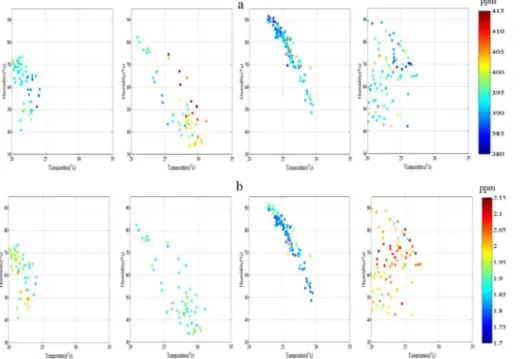
The meteorological parameters (temperature and relative humidity) influenceon trace gases is also examined. Figure 4a and b (top panel corresponds to CO₂ and bottom panel represents CH4) shows the scatter plot of temperature vs. relative humidity as

a function of GHGs during different seasons. Here, dailymean data is used instead of hourly mean data, to avoid the influence of the diurnal variations on correlations. CO₂

20

showed a positive correlation with temperature during all season except during winter. This negative correlation can be attributed to decrease in rate of photosynthesis. IPCC (1990) reports that many mid-latitude plants shows an optimum gross photosynthesis rate when temperature varied from of 20 to 35◦C. The rate of plant respiration tends to be slow below 20◦C. However, at higher temperatures, the respiration rate accelerates

25

rapidly up to a temperature at which, it equals the rate of gross photosynthesis and there can be no net assimilation of carbon. While CH4showed a weak positive

(11)

tem-ACPD

15, 34205–34241, 2015

G. Sreenivas et al.

Title Page

Tables Figures

◭ ◮

Back Close

Full Screen / Esc

Discussion

P

a

per

|

Discussion

P

a

per

|

Discussion

P

a

per

|

Discussion

P

a

per

|

perature does not significantly influence seasonal variation of CH₄(Chen et al., 2015). Seasonal variation of GHG’s also showed an insignificantly negative correlation with relative humidity. A similar observation is also reported by Abhishek et al. (2014). One of the supporting argument can be in humid conditions, these stoma can fully open to increase the uptake of CO2without a net water loss. Also, wetter soils can promote

de-5

composition of dead plant materials, releasing natural fertilizers that help plants grow.

Influence of boundary layer height on GHGs mixing ratios

The planetary boundary layer is the lowest layer of the troposphere where wind speed as a function of temperature plays major role in its thickness variation. It is an important parameter for controlling the observed diurnal variations and potentially masking the

10

emissions signal (Newman et al., 2013). Since complete set of COSMIC RO data is not available during the study period, in this analysis we have analysed RO data from July 2013 to June 2014, along with simultaneous observations of GHG’s. Monthly vari-ations (Figure not show) of BLH computed from high vertical resolution of COSMIC-RO data against CO2 and CH4 concentrations. Monthly BLH is observed to be minimum

15

(maximum) during winter and monsoon (pre monsoon) seasons. The highest (lowest) BLH over study region was identified 3.20 km (1.50 km). An average monthly air tem-perature is maximum (minimum) of 29◦C (20◦C) during summer (winter) months.

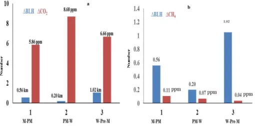
Seasonal change in BLH thickness over study region was observed to be as Mon-soon (M, 1.74 km)<winter (W, 2.10 km)<Post Monsoon (PM, 2.30 km)<Pre-monsoon

20

(Pre-M, 3.15 km); its influence on CO₂and CH₄mixing ratios are shown in Fig. 5a and b. As seasonal BLH thickness increase, mixing ratios of CO2 (CH4) decreased from

8.68 to 5.86 ppm (110 to 40 ppb). The amount of biosphere emissions influence on CO₂and CH₄can be estimated through atmospheric boundary layer processes. Since the study region being a flat terrain variations in CO2and CH4were mostly influenced

25

by boundary layer thickness through convection and biosphere activities.

(12)

ACPD

15, 34205–34241, 2015

G. Sreenivas et al.

Title Page

Tables Figures

◭ ◮

Back Close

Full Screen / Esc

Discussion

P

a

per

|

Discussion

P

a

per

|

Discussion

P

a

per

|

Discussion

P

a

per

|

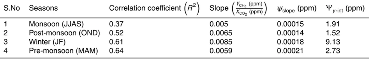
4.4 Correlation between CO2and CH4

A correlation study is carried out between hourly averaged CO2and CH4during all

sea-son for the entire study period. The statistical analysis for different seasons is shown in Table 3. Fang et al. (2015) suggest that correlation coefficient (R) value higher than 0.50 indicates similar source mechanism of CO2and CH4. Also, a positive correlation

5

dominance of anthropogenic emission on carbon cycle. Our study also reveals a strong positive correlation observed between CO2and CH4during winter, pre-monsoon,

mon-soon and post-monmon-soon withR equal to 0.80, 0.80, 0.61 and 0.72 respectively. Sea-sonal regression coefficients (slope) and their uncertainties (ψ_slope, ψ_y_-int) are com-puted using Taylor (1997) which showed maximum during winter, pre-monsoon and

10

minimum in monsoon that figure out the hourly stability of the mixing ratios between CO2and CH4. This can be due to relatively simple source/sink process of CO2in

com-parison with CH₄. Dilution effects during transport of CH₄and CO₂ can be minimized to some extent by dividing the increase of CH4over time by the respective increase in

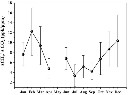
CO2 (Worthy et al., 2009). Figure 6 shows the seasonal variation of∆CH4/∆CO2. In

15

this study, background concentration of respective GHG’s are determined as mean val-ues of the 1.25 percentile of data for monsoon, post-monsoon, pre-monsoon and winter (Pan et al., 2011; Worthy et al., 2009). Annual∆CH4/∆CO2over the study region

dur-ing the study period is found to be 7.1 (ppb ppm−1). This low value clearly indicates the dominance of CO2over the study region. The reported∆CH4/∆CO2values from some

20

of the rural sites viz Canadian Arctic and Hateruma Island (China) is of the order 12.2 and ∼10 ppb ppm−1 respectively (Worthy et al., 2009; Tohjima et al., 2014). Average

∆CH4/∆CO2ratio during winter, pre-monsoon, monsoon and post-monsoon are 9.40,

6.40, 4.40, and 8.20 ppb respectively. Monthly average, of ∆CH4/∆CO2, is relatively

high from late post-monsoon to winter, when the biotic activity is relatively dormant

25

(Tohjima et al., 2014). During pre-monsoon decease in ∆CH4/∆CO2 ratio indicates

(13)

ACPD

15, 34205–34241, 2015

G. Sreenivas et al.

Title Page

Tables Figures

◭ ◮

Back Close

Full Screen / Esc

Discussion

P

a

per

|

Discussion

P

a

per

|

Discussion

P

a

per

|

Discussion

P

a

per

|

4.5 Methane (CH4) sink mechanism

Methane (CH4) is the most powerful greenhouse gas after CO2in the atmosphere due

to its strong positive radiative forcing (IPCC, 1990; Stocker et al., 2013). Atmospheric CH4 is mainly (70–80 %) from biological origin produced in anoxic environments, by

anaerobic digestion of organic matter (Crutzen and Zimmermann, 1991). The major

5

CH₄ sink is oxidation by hydroxyl radicals (OH), which accounts for 90 % of CH₄ sink (Vaghjiani and Ravishankara, 1991; Kim et al., 2015). OH radicals are very reactive and are responsible for the oxidation of almost all gases in the atmosphere. Primary source for OH radical formation in the atmosphere is photolysis of ozone (O₃) and water vapor (H₂O). Eisele et al. (1997) defined primary and secondary source of OH radicals in the

10

atmosphere. Primary source of OH radical is as follows;

O₃+hν(λ≤310 nm) → O₂+O(1D) where O(1D) is electronically excited atom. (R1)

O(1D)+O₂ → O+M (R2)

O(1D)+H2O → 2OH primary OH formation. (R3)

Removal of CH4 is constrained by the presence of OH radicals in the atmosphere.

15

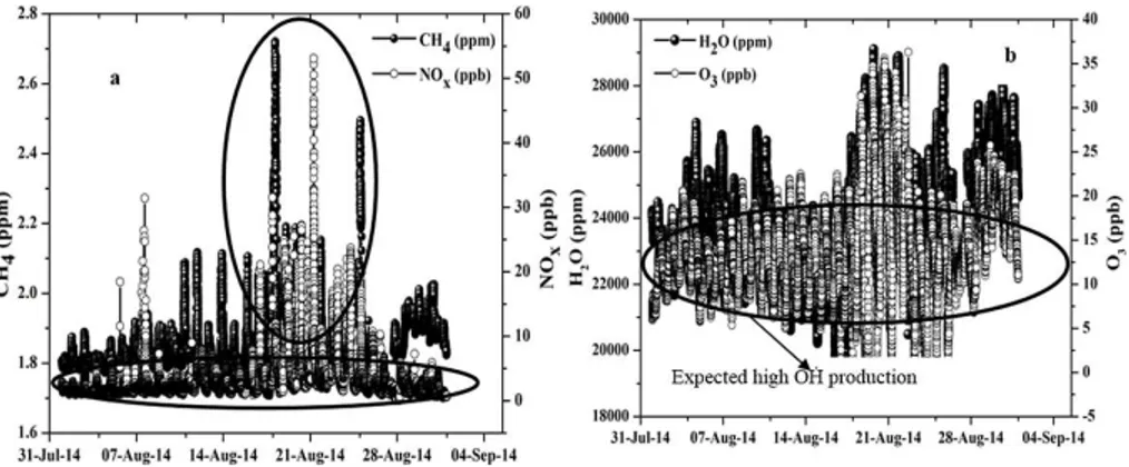
A 1 min time series analysis of CH4, NOx, O3 and H2O and associated wind vector

for August 2014 to understand the CH4 chemistry is shown in Fig. 7a and b. Low

NO_x (1–2 ppb) values are shown in horizontal elliptical region of Fig. 7a and observed corresponding low CH4(1.80 ppm) concentrations. The low NOxin turn produces high OH radicals in the atmosphere due to conversion of HO2radical by NO, which removes

20

CH₄through oxidation process as shown below.

HO2+NO → O ˙H+NO2 when NOxlevels 1–2 ppb (R4)

CH4+O ˙H → C ˙H3+H2O main CH4removal process (R5)

NO2+OH+M → HNO3+M if NOx>2 ppb (OH↓, CH4↑) (R6)

Crutzen and Zimmermann (1991) and Eisele et al. (1997) observed that at low NO_x

25

(14)

ACPD

15, 34205–34241, 2015

G. Sreenivas et al.

Title Page

Tables Figures

◭ ◮

Back Close

Full Screen / Esc

Discussion

P

a

per

|

Discussion

P

a

per

|

Discussion

P

a

per

|

Discussion

P

a

per

|

react with NO to form OH radicals. Therefore OH radicals are much higher in the case of low NOx. When NOx levels increase more than 2 ppb, most of the OH radicals react with NO2to form nitric acid (HNO3). In first order, the levels of CH4in the atmosphere

depend on the levels of NO_x though the production of OH radicals in the atmosphere is still uncertain. Figure 7a and b showed high CH4, H2O, O3 and NOx during a few

5

days in August 2014. High concentrations of CH4, NOx and other gases are observed in the eastern direction of study site. Very high NO_xlevels above 10 ppb are observed and subsequently CH4 concentrations also increased to 2.40 from 1.80 ppm. In the

eastern direction of study site a national highway and single line broad gauge railway network are present which act as possible sources of NO_x, CH₄ and CO₂. Increase

10

in emissions of NO_x causes decline in the levels of OH radicals and subsequently observed high CH4over the study region.

4.6 Influence of vegetation on GHG’s.

In India cropping season is classified into (i) Kharif and (ii) Rabi based on the onset of monsoon. The kharif season is from July to October during the south-west

mon-15

soon and Rabi season is from October to March (Koshal, 2013). NDVI being one of the indicators of vegetation change, monthly variations of CO₂ and CH₄ against NDVI is studied to understand the impact of land use land cover on mixing ratios of CO2 and CH4. Monthly changes in NDVI, CO2 and CH4 are shown in Fig. 8. Monthly

mean of GHG’s represented in this analysis is calculated from daily day time (10:00–

20

16:00 LT) mean. Maximum NDVI of 0.60 corresponding to the minimum CO₂ concentra-tion (about 382 ppm) is observed in September. NDVI showed inverse relaconcentra-tionship with CO2, mainly due to change in vegetation which affects the CO2 concentrations. CH4

and NDVI values follow similar trends with highest CH₄concentrations in October 2014 (about 2.05 ppm) and minimum about 1.80 ppm in July 2014. The main source for CH4

25

(15)

ACPD

15, 34205–34241, 2015

G. Sreenivas et al.

Title Page

Tables Figures

◭ ◮

Back Close

Full Screen / Esc

Discussion

P

a

per

|

Discussion

P

a

per

|

Discussion

P

a

per

|

Discussion

P

a

per

|

controls the soil emissions of CO₂, CH₄ are moisture content, soil temperature, veg-etation and soil respiration (Smith et al., 2003; Jones et al., 2005; Chen et al., 2010) respectively.

Biomass burning (forest fire and crop residue burning) is one of the major sources of gaseous pollutants such as carbon monoxide (CO), methane (CH4), nitrous oxides

5

(NO_x) and hydrocarbons in the troposphere (Crutzen et al., 1990, 1985; Sharma et al., 2010). In order to study the role of biomass burning on GHG’s over study site we have analysed GHG’s emissions from biomass burning using long term (2003–2013) Fire Energetics and Emissions Research version 1.0 (FEER v1) data. Emission co-efficient (C_e) products during biomass burring is developed from coincident

measure-10

ments of fire radiative power (FRP) and AOD from MODIS Aqua and Terra satellites (Ichoku and Ellison, 2014). Figure 10 shows seasonal variation of CO2 emission due

to biomass burning over the study site. Enhancement in CO2 emission is seen during

pre-monsoon months; which also supports earlier observation (Fig. 2a). This analysis reveals that biomass burning has a role in pre-monsoon enhancement of CO2 over

15

study site. For a qualitative analysis of this long range transport, we have analysed air mass trajectories ending over study site during different seasons.

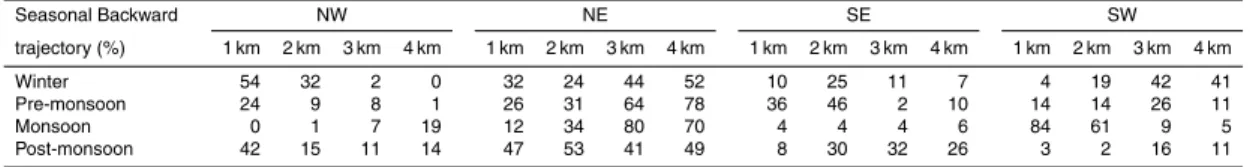
4.7 Long range circulations

To understand the role of long range circulation we separated the trajectory into 4 clus-ters based on their pathway, namely North-East (N-E), North-West (N-W), South-East

20

(S-E), South-West (S-W). The main criterion of trajectory clustering is to minimize the variability among trajectories and maximize variability among clusters. Cluster mean trajectories of air mass and their percentage contribution to the total calculated for each season over the study period at 3 km altitude are depicted in Fig. 9. Majority of air mass trajectories during winter (∼44 %), pre-monsoon (∼64 %), monsoon (∼80 %)

25

and post-monsoon (∼41 %) are originating from NW parts of the study site. For a com-prehensive analysis, percentage occurrences of cluster mean trajectories of air mass over study area during different season at different altitudes are also tabulated in

(16)

ACPD

15, 34205–34241, 2015

G. Sreenivas et al.

Title Page

Tables Figures

◭ ◮

Back Close

Full Screen / Esc

Discussion

P

a

per

|

Discussion

P

a

per

|

Discussion

P

a

per

|

Discussion

P

a

per

|

ble 4. During post-monsoon to early pre-monsoon periods which are generally the post-harvest period for some of the crops agriculture residue burning which are quite common in the NW and NE regions part of India (Sharma et al., 2010).Our analysis reveals that during this period majority of air mass reaching the study site at different altitudes come from this part of the country.

5

5 Conclusions

The present study analysed the seasonal variations of atmospheric GHG’s (CO2 and

CH₄) and associated prevailing meteorology over Shadnagar, a suburban site of Cen-tral India during the period 2014. The salient findings of the study are the following:

– The annual mean of CO2and CH4over the study region is found to be 394±2.92

10

and 1.92±0.07 ppm (µ±1σ) respectively. CO₂ and CH₄ showed a significant seasonal variation during the study period. Maximum (Minimum) CO₂ is ob-served during Pre-monsoon (Monsoon), while CH4 recorded maximum during

post-monsoon and minimum in monsoon. Seasonal analysis of FEER data also showed maximum emission of CO₂due to biomass burning during pre-monsoon

15

months which indicates the influence of biomass burning on local emissions.

– CO2and CH4showed consistent diurnal behavior in spite of their significant

sea-sonal variations, with an observed morning (06:00 IST) maxima, followed by af-ternoon minima (14:00 IST) and enhancing in the late evening (∼22:00 IST).

– Correlation coefficient (R) between wind speed and CO2 during pre-monsoon,

20

monsoon, post-monsoon and winter is 0.56, 0.32, 0.06 and 0.67 respectively. While for CH4 it is found be 0.28, 0.71, 0.21, and 0.60 respectively. Negative

correlation indicates that the influence of local sources on GHG’s, however, poor correlation coefficients during different seasons suggest the role of regional/local transport.

(17)

ACPD

15, 34205–34241, 2015

G. Sreenivas et al.

Title Page

Tables Figures

◭ ◮

Back Close

Full Screen / Esc

Discussion

P

a

per

|

Discussion

P

a

per

|

Discussion

P

a

per

|

Discussion

P

a

per

|

– CO₂ showed a positive correlation with temperature during all seasons except during winter. Whereas CH4showed a weak positive correlation with temperature

during pre-monsoon and post-monsoon, while showing a weak negative correla-tion during monsoon and winter.

– CO2 and CH4 showed a strong positive correlation during winter, pre-monsoon,

5

monsoon and post-monsoon with R equal to 0.80, 0.80, 0.61 and 0.72 respec-tively. This clearly indicates the seasonal variations in source-sink mechanisms of CO₂and CH₄respectively.

– Presence of OH radicals has been implicitly confirmed as a major sink of CH4

over the study region.

10

Acknowledgement. This work was part of the Atmospheric CO₂ Retrieval and Monitoring

(ACRM) under National Carbon Project (NCP) of ISRO-GBP. We thank D & PQE division of NRSC and P. Sujatha, ACSG for sharing AWS and boundary layer data. The authors sincerely thank the AT-CTM project of ISRO-GBP for providing the O₃and NO_xanalyzers. We would also like to thank MODIS and COSMIC team for providing scientific data sets used in this study.

15

References

Ao, C. O., Waliser, D. E., Chan, S. K., Li, J. L., Tian, B., Xie, F., and Mannucci, A. J.: Plane-tary boundary layer heights from GPS radio occultation refractivity and humidity profiles, J. Geophys. Res.-Atmos., 117, D16117, doi:10.1029/2012JD017598, 2012.

Baer, D. S., Paul, J. B., Gupta, M., and O’Keefe, A.: Sensitive absorption measurements in

20

the near-infrared region using off-axis integrated cavity output spectroscopy, in: International Symposium on Optical Science and Technology, International Society for Optics and Pho-tonics, 167–176, 2002.

Berman, E. S., Fladeland, M., Liem, J., Kolyer, R., and Gupta, M.: Greenhouse gas analyzer for measurements of carbon dioxide, methane, and water vapor aboard an unmanned aerial

25

vehicle, Sensor. Actuat. B-Chem., 169, 128–135, 2012.

(18)

ACPD

15, 34205–34241, 2015

G. Sreenivas et al.

Title Page

Tables Figures

◭ ◮

Back Close

Full Screen / Esc

Discussion

P

a

per

|

Discussion

P

a

per

|

Discussion

P

a

per

|

Discussion

P

a

per

|

Chen, H., Wu, N., Wang, Y., and Peng, C.: Methane is an Important Greenhouse Gas. Methane Emissions from Unique Wetlands in China: Case Studies, Meta Analyses and Modelling, Ch. 1, Higher Education Press and Walter de Gruyter GmbH, Berlin/Boston, ISBN 978-3-11-030021-5, 2015.

Crutzen, P. J. and Andreae, M. O.: Biomass burning in the tropics: impact on atmospheric

5

chemistry and biogeochemical cycles, Science, 250, 1669–1678, 1990.

Crutzen, P. J., Delany, A. C., Greenberg, J., Haagenson, P., Heidt, L., Lueb, R., Pollock, W., Seiler, W., Wartburg, A., and Zimmerman, P.: Tropospheric chemical composition measure-ments in Brazil during the dry season, J. Atmos. Chem., 2, 233–256, 1985.

Draxler, R. R. and Rolph, G. D.: HySPLIT (Hybrid Single Particle Lagrangian Integrated

Tra-10

jectory) Model access via NOAA ARL READY website, available at: http://www.arl.noaa.gov/ ready/hysplit4.html (last access: 31 December 2014), NOAA Air Resources Laboratory, Sil-ver Spring, MD, 2003.

Eisele, F. L., Mount, G. H., Tanner, D., Jefferson, A., Shetter, R., Harder, J. W., and Williams, E. J.: Understanding the production and interconversion of the hydroxyl radical

dur-15

ing the Tropospheric OH Photochemistry Experiment, J. Geophys. Res.-Atmos., 102, 6457– 6465, 1997.

Fang, S. X., Zhou, L. X., Tans, P. P., Ciais, P., Steinbacher, M., Xu, L., and Luan, T.: In situ measurement of atmospheric CO₂at the four WMO/GAW stations in China, Atmos. Chem. Phys., 14, 2541–2554, doi:10.5194/acp-14-2541-2014, 2014.

20

Fang, S. X., Tans, P. P., Steinbacher, M., Zhou, L. X., and Luan, T.: Study of the regional CO₂ mole fractions filtering approach at a WMO/GAW regional station in China, Atmos. Meas. Tech. Discuss., 8, 7057–7091, doi:10.5194/amtd-8-7057-2015, 2015.

Fearnside, P. M.: Global warming and tropical land-use change: greenhouse gas emissions from biomass burning, decomposition and soils in forest conversion, shifting cultivation and

25

secondary vegetation, Climatic Change, 46, 115–158, 2000.

Frankenberg, C., Bergamaschi, P., Butz, A., Houweling, S., Meirink, J. F., Notholt, J., Pe-tersen, A. K., Schrijver, H., Warneke, T., and Aben, I.: Tropical methane emissions: a re-vised view from SCIAMACHY onboard ENVISA T, Geophys. Res. Lett., 35, L15811, doi:10.1029/2008GL034300, 2008.

30

(19)

ACPD

15, 34205–34241, 2015

G. Sreenivas et al.

Title Page

Tables Figures

◭ ◮

Back Close

Full Screen / Esc

Discussion

P

a

per

|

Discussion

P

a

per

|

Discussion

P

a

per

|

Discussion

P

a

per

|

Gaur, A., Tripathi, S. N., Kanawade, V. P., Tare, V., and Shukla, S. P.: Four-year measurements of trace gases (SO₂, NO_x, CO, and O₃) at an urban location, Kanpur, in Northern India, J. Atmos. Chem., 71, 283–301, 2014.

Gilmanov, T. G., Johnson, D. A., Saliendra, N. Z., Akshalov, K., and Wylie, B. K.: Gross primary productivity of the true steppe in Central Asia in relation to NDVI: scaling up CO₂ fluxes,

5

Environ. Manage., 33, 492–508, 2004.

Goroshi, S. K., Singh, R. P., Panigrahy, S., and Parihar, J. S.: Analysis of seasonal variability of vegetation and methane concentration over India using SPOT-VEGETATION and ENVISAT-SCIAMACHY data, Journal of the Indian Society of Remote Sensing, 39, 315–321, 2011. Hassan, A. G. A.: Diurnal and monthly variations in atmospheric CO₂ level in Qena, Upper

10

Egypt, Resources and Environment, 5, 59–65, 2015.

Ichoku, C. and Ellison, L.: Global top-down smoke-aerosol emissions estimation using satellite fire radiative power measurements, Atmos. Chem. Phys., 14, 6643–6667, doi:10.5194/acp-14-6643-2014, 2014.

IPCC: Climate Change: The IPCC Scientific Assessment, edited by: Houghton, J. T.,

15

Jerkins, G. J., and Ephraums, J. J., Cambridge University Press, New York, 1990.

James, M. E. and Kalluri, S. N.: The Pathfinder AVHRR land data set: an improved coarse resolution data set for terrestrial monitoring, Int. J. Remote Sens., 15, 3347–3363, 1994. Jones, C., McConnell, C., Coleman, K., Cox, P., Falloon, P., Jenkinson, D., and Powlson, D.:

Global climate change and soil carbon stocks; predictions from two contrasting models for

20

the turnover of organic carbon in soil, Glob. Change Biol., 11, 154–166, 2005.

Keppler, F., Hamilton, J. T., Braß, M. and Röckmann, T.: Methane emissions from terrestrial plants under aerobic conditions, Nature, 439, 187–191, 2006.

Kim, H. S., Chung, Y. S., Tans, P. P., and Dlugokencky, E. J.: Decadal trends of atmospheric methane in East Asia from 1991 to 2013, Air Quality, Atmosphere and Health, 8, 293–298,

25

2015.

King, M. D., Kaufman, Y. J., Menzel, W. P., and Tanre, D.: Remote sensing of cloud, aerosol, and water vapor properties from the Moderate Resolution Imaging Spectrometer (MODIS), IEEE T. Geosci. Remote , 30, 2–27, 1992.

Kirschke, S., Bousquet, P., Ciais, P., Saunois, M., Canadell, J. G., Dlugokencky, E. J.,

Bergam-30

aschi, P., Bergmann, D., Blake, D. R., Bruhwiler, L., Cameron-Smith, P., Castaldi, S., Cheval-lier, F., Feng, L., Fraser, A., Heimann, M., Hodson, E. L., Houweling, S., Josse, B., Fraser, P. J., Krummel, P. B., Lamarque, J.-F., Langenfelds, R. L., Quéré, C. L., Naik, V., O’Doherty,

(20)

ACPD

15, 34205–34241, 2015

G. Sreenivas et al.

Title Page

Tables Figures

◭ ◮

Back Close

Full Screen / Esc

Discussion

P

a

per

|

Discussion

P

a

per

|

Discussion

P

a

per

|

Discussion

P

a

per

|

S., Palmer, P. I., Pison, I., Plummer, D., Poulter, B., Prinn, R. G., Rigby, M., Ringeval, B., San-tini, M., Schmidt, M., Shindell, D. T., Simpson, I. J., Spahni, R., Steele, L. P., Strode, S. A., Sudo, K., Szopa, S., van der Werf, G. R., Voulgarakis, A., Weele, M., Weiss, R. F., Williams, J. E., and Guang, Z.: Three decades of global methane sources and sinks, Nat. Geosci., 6, 813–823, doi:10.1038/NGEO1955, 2013.

5

Koshal, A. K.: Spatial temporal climatic change variability of cropping system in western Uttar Pradesh, Int. J. Remote Sens. Geosci., 2, 36–45, 2013.

Lewis, A. C., Evans, M. J., Hopkins, J. R., Punjabi, S., Read, K. A., Purvis, R. M., Andrews, S. J., Moller, S. J., Carpenter, L. J., Lee, J. D., Rickard, A. R., Palmer, P. I., and and Parrington, M.: The influence of biomass burning on the global distribution of selected non-methane organic

10

compounds, Atmos. Chem. Phys., 13, 851–867, doi:10.5194/acp-13-851-2013, 2013. Machida, T., Kita, K., Kondo, Y., Blake, D., Kawakami, S., Inoue, G., and T. Ogawa.: Vertical and

meridional distributions of the atmospheric CO₂ mixing ratio between northern midlatitudes and southern subtropics, J. Geophys. Res.-Atmos., 107, 1984–2012, 2002.

Mahesh, P., Sharma, N., Dadhwal, V. K., Rao, P. V. N., and Apparao, B. V.: Impact of land–sea

15

breeze and rainfall on CO₂variations at a coastal station, J. Earth Sci. Clim. Change, 5, 201, doi:10.4172/2157-7617.1000201, 2014.

Mahesh, P., Sreenivas, G., Rao, P. V. N., Dadhwal, V. K., Sai Krishna, S. V. S., and Mallikar-jun, K.: High precision surface level CO₂ and CH₄ using Off-Axis Integrated Cavity Out-put Spectroscopy (OA-ICOS) over Shadnagar, India, Int. J. Remote Sens., 36, 5754–5765,

20

doi:10.1080/01431161.2015.1104744, 2015.

Miller, J. B., Gatti, L. V., d’Amelio, M. T. S., Crotwell, A. M., Dlugokencky, E. J., Bakwin, P., Artaxo, P., and Tans, P. P.: Airborne measurements indicate large methane emissions from the eastern Amazon basin, Geophys. Res. Lett., 34, L10809, doi:10.1029/2006GL029213, 2007.

25

Monastersky, R.: Global carbon dioxide levels near worrisome milestone, Nature, 497, 13–14, 2013.

Newman, S., Jeong, S., Fischer, M. L., Xu, X., Haman, C. L., Lefer, B., Alvarez, S., Rap-penglueck, B., Kort, E. A., Andrews, A. E., Peischl, J., Gurney, K. R., Miller, C. E., and Yung, Y. L.: Diurnal tracking of anthropogenic CO₂ emissions in the Los Angeles basin

30

(21)

ACPD

15, 34205–34241, 2015

G. Sreenivas et al.

Title Page

Tables Figures

◭ ◮

Back Close

Full Screen / Esc

Discussion

P

a

per

|

Discussion

P

a

per

|

Discussion

P

a

per

|

Discussion

P

a

per

|

Nishanth, T., Praseed, K. M., Satheesh Kumar, M. K., and Valsaraj, K. T.: Observational study of surface O₃, NO_x, CH₄ and total NMHCs at Kannur, India, Aerosol Air Qual. Res., 14, 1074–1088, 2014.

Pan, X. L., Kanaya, Y., Wang, Z. F., Liu, Y., Pochanart, P., Akimoto, H., Sun, Y. L., Dong, H. B., Li, J., Irie, H., and Takigawa, M.: Correlation of black carbon aerosol and carbon monoxide

5

in the high-altitude environment of Mt. Huang in Eastern China, Atmos. Chem. Phys., 11, 9735–9747, doi:10.5194/acp-11-9735-2011, 2011.

Patil, M. N., Dharmaraj, T., Waghmare, R. T., Prabha, T. V., and Kulkarni, J. R.: Measurements of carbon dioxide and heat fluxes during monsoon-2011 season over rural site of India by eddy covariance technique, J. Earth Syst. Sci., 123, 177–185, 2014.

10

Paul, J. B., Lapson, L., and Anderson, J. G.: Ultrasensitive absorption spectroscopy with a high-finesse optical cavity and off-axis alignment, Appl. Optics, 40, 4904–4910, 2001.

Pielke, R. A., Marland, G., Betts, R. A., Chase, T. N., Eastman, J. L., Niles, J. O., and Running, S. W.: The influence of land-use change and landscape dynamics on the climate system: relevance to climate-change policy beyond the radiative effect of greenhouse gases, Philos.

15

T. Roy. Soc. A, 360, 1705–1719, 2002.

Ramachandran, S. and Rajesh, T. A.: Black carbon aerosol mass concentrations over Ahmedabad, an urban location in western India: comparison with urban sites in Asia, Europe, Canada, and the United States, J. Geophys. Res.-Atmos., 112, D06211, doi:10.1029/2006JD007488, 2007.

20

Salomonson, V. V., Barnes, W. L., Maymon, P. W., Montgomery, H. E., and Ostrow, H.: MODIS: Advanced facility instrument for studies of the Earth as a system, IEEE T. Geosci. Remote, 27, 145–153, 1989.

Schneising, O., Buchwitz, M., Burrows, J. P., Bovensmann, H., Bergamaschi, P., and Peters, W.: Three years of greenhouse gas column-averaged dry air mole fractions retrieved from

satel-25

lite – Part 2: Methane, Atmos. Chem. Phys., 9, 443–465, doi:10.5194/acp-9-443-2009, 2009. Anu Rani Sharma, Shailesh Kumar Kharol, Badarinath, K. V. S., and Darshan Singh: Impact of

agriculture crop residue burning on atmospheric aerosol loading –a study over Punjab State, India, Ann. Geophys., 28, 367–379, doi:10.5194/angeo-28-367-2010, 2010.

Sharma, N., Nayak, R. K., Dadhwal, V. K., Kant, Y., and Ali, M. M.: Temporal variations of

30

atmospheric CO₂ in Dehradun, India during 2009, Air, Soil and Water Res., 6, 37–45, doi:10.4137/ASWR.S10590, 2013.

(22)

ACPD

15, 34205–34241, 2015

G. Sreenivas et al.

Title Page

Tables Figures

◭ ◮

Back Close

Full Screen / Esc

Discussion

P

a

per

|

Discussion

P

a

per

|

Discussion

P

a

per

|

Discussion

P

a

per

|

Sharma, N., Dadhwal, V. K., Kant, Y., Mahesh, P., Mallikarjun, K., Gadavi, H., Sharma, A., and Ali, M. M.: Atmospheric CO₂Variations in Two Contrasting Environmental Sites Over India, Air, Soil and Water Res., 7, 61–68, doi:10.4137/ASWR.S13987, 2014.

Smith, K. A., Ball, T., Conen, F., Dobbie, K. E., Massheder, J., and Rey, A.: Exchange of green-house gases between soil and atmosphere: interactions of soil physical factors and biological

5

processes, Eur. J. Soil Sci., 54, 779–791, 2003.

Stocker, T. F., Qin, D., Plattner, G. K., Alexander, L. V., Allen, S. K., Bindoff, N. L., Bréon, F. M., Church, J. A., Cubasch, U., Emori, S., Forster, P., Friedlingstein, P., Gillett, N., Gre-gory, J. M., Hartmann, D. L., Jansen, E., Kirtman, B., Knutti, R., Krishna Kumar, K., Lemke, P., Marotzke, J., Masson-Delmotte, V., Meehl, G. A., Mokhov, I. I., Piao, S., Ramaswamy, V.,

10

Randall, D., Rhein, M., Rojas, M., Sabine, C., Shindell, D., Talley, L. D., Vaughan D. G., and Xie, S. P.: Technical summary, in: Climate Change 2013: The Physical Science Basis, Con-tribution of Working Group I to the Fifth Assessment Report of the Intergovernmental Panel on Climate Change, edited by: Stocker, T. F., Qin, D., Plattner, G.-K., Tignor, M., Allen, S. K., Boschung, J., Nauels, A., Xia, Y., Bex, V., and Midgley, P. M., Cambridge University Press,

15

Cambridge, UK and New York, NY, USA, 2013.

Stohl, A., Hittenberger, M., and Wotawa, G.: Validation of the Lagrangian particle dispersion model FLEXPART against large-scale tracer experiment data, Atmos. Environ., 32, 4245– 4264, 1998.

Taylor, J.: An Introduction to Error Analysis: The Study of Uncertainties in Physical

Measure-20

ment, University Science Books, Sausalito, CA, 1997.

Thum, T., Aalto, T., Laurila, T., Aurela, M., Hatakka, J., Lindroth, A., and Vesala, T.: Spring initiation and autumn cessation of boreal coniferous forest CO₂exchange assessed by me-teorological and biological variables, Tellus B, 61, 701–717, 2009.

Tohjima, Y., Kubo, M., Minejima, C., Mukai, H., Tanimoto, H., Ganshin, A., Maksyutov, S.,

Kat-25

sumata, K., Machida, T., and Kita, K.: Temporal changes in the emissions of CH₄ and CO from China estimated from CH₄/CO₂ and CO/CO₂ correlations observed at Hateruma Is-land, Atmos. Chem. Phys., 14, 1663–1677, doi:10.5194/acp-14-1663-2014, 2014.

Vaghjiani, G. L. and Ravishankara, A. R.: New measurement of the rate coefficient for the reaction of OH with methane, Nature, 350, 406–409, 1991.

30

(23)

ACPD

15, 34205–34241, 2015

G. Sreenivas et al.

Title Page

Tables Figures

◭ ◮

Back Close

Full Screen / Esc

Discussion

P

a

per

|

Discussion

P

a

per

|

Discussion

P

a

per

|

Discussion

P

a

per

|

Worthy, D. E. J., Chan, E., Ishizawa, M., Chan, D., Poss, C., Dlugokencky, E. J., Maksyutov, S., and Levin, I.: Decreasing anthropogenic methane emissions in Europe and Siberia inferred from continuous carbon dioxide and methane observations at Alert, Canada, J. Geophys. Res.-Atmos., 114, D10301, doi:10.1029/2008JD011239, 2009.

Yang, L., Wang, X., Guo, M., Tani, H., Matsuoka, N., and Matsumura, S.: Spatial and

tem-5

poral relationships among NDVI, climate factors, and land cover changes in Northeast Asia from 1982 to 2009, GIScience and Remote Sensing, 48, 371–393, doi:10.2747/1548-1603.48.3.371, 2011.

Yunck, T. P., Liu, C.-H., and Ware, R.: A history of GPS sounding, Terr. Atmos. Ocean Sci., 11, 1–20, 2000.

10

(24)

ACPD

15, 34205–34241, 2015

G. Sreenivas et al.

Title Page

Tables Figures

◭ ◮

Back Close

Full Screen / Esc

Discussion

P

a

per

|

Discussion

P

a

per

|

Discussion

P

a

per

|

Discussion

P

a

per

|

Table 1.Data used.

Sensor Period Parameter resolution Source

GGA-24EP Jan 2014 to Dec 2014 CO2,CH4and H2O 1 Hz time ASL, NRSC 42i-NO-NO2-NOx Jul 2014 to Sep 2014 NOx(=NO+NO2) 1 min time ASL, NRSC 49i-O3 Jul 2014 to Sep 2014 O3 1 min time ASL, NRSC AWS Jan 2014 to Dec 2014 WS, WD, AT, RH 60 min time NRSC

Terra/MODIS Jan 2014 to Dec 2014 NDVI 5 km horizontal http://ladsweb.nascom.nasa.gov/data/search.html COSMIC-1DVAR Jul 2013 to Jun 2014 Refractivity (N) 0.1 km vertical

(25)

ACPD

15, 34205–34241, 2015

G. Sreenivas et al.

Title Page

Tables Figures

◭ ◮

Back Close

Full Screen / Esc

Discussion

P

a

per

|

Discussion

P

a

per

|

Discussion

P

a

per

|

Discussion

P

a

per

|

Table 2.Seasonal amplitudes of CO₂and CH₄ over study region arriving from different

direc-tions.

Wind Direction WinterCO2

CH4(ppm) Pre-monsoon

CO2

CH4(ppm) Monsoon

CO2

CH4(ppm) Post-monsoon

CO2

CH4(ppm)

0–45 399.85/1.98 410.37/1.94 400.72/1.91 395.13/2.02

45–90 391.66/1.94 399.59/1.89 388.82/1.91 390.23/1.98

90–135 391.57/1.93 397.79/1.87 388.99/1.87 389.06/1.97 135–180 389.34/1.89 393.87/1.85 391.81/1.86 387.69/1.97 180–225 391.14/1.89 396.75/1.85 390.28/1.82 392.30/2.02 225–270 389.13/1.88 394.81/1.86 390.26/1.82 384.40/1.94 270–315 388.68/1.87 398.68/1.89 389.58/1.82 384.99/1.93 315–360 390.87/1.91 401.17/1.89 387.58/1.83 389.32/1.98

(26)

ACPD

15, 34205–34241, 2015

G. Sreenivas et al.

Title Page

Tables Figures

◭ ◮

Back Close

Full Screen / Esc

Discussion

P

a

per

|

Discussion

P

a

per

|

Discussion

P

a

per

|

Discussion

P

a

per

|

Table 3.Statistical correlation between CO₂and CH₄.

S.No Seasons Correlation coefficientR2 SlopeYCH4(ppm)

X_CO2(ppm)

ψslope(ppm) Ψy-int(ppm)

1 Monsoon (JJAS) 0.37 0.005 0.00015 1.91

2 Post-monsoon (OND) 0.52 0.0065 0.00014 1.52

3 Winter (JF) 0.61 0.0085 0.00018 9.13

(27)

ACPD

15, 34205–34241, 2015

G. Sreenivas et al.

Title Page

Tables Figures

◭ ◮

Back Close

Full Screen / Esc

Discussion

P

a

per

|

Discussion

P

a

per

|

Discussion

P

a

per

|

Discussion

P

a

per

|

Table 4.Cluster analysis of air mass trajectories reaching Shadnagar at various heights during

different seasons.

Seasonal Backward NW NE SE SW

trajectory (%) 1 km 2 km 3 km 4 km 1 km 2 km 3 km 4 km 1 km 2 km 3 km 4 km 1 km 2 km 3 km 4 km

Winter 54 32 2 0 32 24 44 52 10 25 11 7 4 19 42 41

Pre-monsoon 24 9 8 1 26 31 64 78 36 46 2 10 14 14 26 11

Monsoon 0 1 7 19 12 34 80 70 4 4 4 6 84 61 9 5

Post-monsoon 42 15 11 14 47 53 41 49 8 30 32 26 3 2 16 11

(28)

ACPD

15, 34205–34241, 2015

G. Sreenivas et al.

Title Page

Tables Figures

◭ ◮

Back Close

Full Screen / Esc

Discussion

P

a

per

|

Discussion

P

a

per

|

Discussion

P

a

per

|

Discussion

P

a

per

|

Figure 1. (a)Schematic representation of study area;(b–e)Seasonal variation of prevailing

(29)

ACPD

15, 34205–34241, 2015

G. Sreenivas et al.

Title Page

Tables Figures

◭ ◮

Back Close

Full Screen / Esc

Discussion

P

a

per

|

Discussion

P

a

per

|

Discussion

P

a

per

|

Discussion

P

a

per

|

Figure 2. (a–b)Seasonal variations of CO₂and CH₄;(c–d)diurnal variations of CO₂and CH₄

during 2014.

(30)

ACPD

15, 34205–34241, 2015

G. Sreenivas et al.

Title Page

Tables Figures

◭ ◮

Back Close

Full Screen / Esc

Discussion

P

a

per

|

Discussion

P

a

per

|

Discussion

P

a

per

|

Discussion

P

a

per

|

(31)

ACPD

15, 34205–34241, 2015

G. Sreenivas et al.

Title Page

Tables Figures

◭ ◮

Back Close

Full Screen / Esc

Discussion

P

a

per

|

Discussion

P

a

per

|

Discussion

P

a

per

|

Discussion

P

a

per

|

Figure 4. (a)Seasonal variation of CO₂ as function of humidity and temperature during

win-ter, pre-monsoon, monsoon and post-monsoon.(b) Seasonal variation of CH₄ as function of humidity and temperature during respective seasons.

(32)

ACPD

15, 34205–34241, 2015

G. Sreenivas et al.

Title Page

Tables Figures

◭ ◮

Back Close

Full Screen / Esc

Discussion

P

a

per

|

Discussion

P

a

per

|

Discussion

P

a

per

|

Discussion

P

a

per

|

(33)

ACPD

15, 34205–34241, 2015

G. Sreenivas et al.

Title Page

Tables Figures

◭ ◮

Back Close

Full Screen / Esc

Discussion

P

a

per

|

Discussion

P

a

per

|

Discussion

P

a

per

|

Discussion

P

a

per

|

Figure 6.Monthly variation of∆CH₄/∆CO₂during study period.

(34)

ACPD

15, 34205–34241, 2015

G. Sreenivas et al.

Title Page

Tables Figures

◭ ◮

Back Close

Full Screen / Esc

Discussion

P

a

per

|

Discussion

P

a

per

|

Discussion

P

a

per

|

Discussion

P

a

per

|