Prescription Patterns of Pharmaceuticals Ana Sofia Oliveira Gonçalves 543 Masters in Economics

(1)

A Work Project, presented as part of the requirements for the Award of a Master’s Degree in Economics from the NOVA – School of Business and Economics

Prescription Patterns of Pharmaceuticals

Ana Sofia Oliveira Gonçalves #543

Masters in Economics

A Project carried out on the area of Applied Policy Analysis under the supervision of Professor Pedro Pita Barros

(2)

2

Abstract

In May 2011, Portugal signed the Memorandum of Understanding in which it guarantees a reduction in the public spending on pharmaceuticals. The aim of this research work is to analyse the possibility of hospital cost

reductions in HIV, oncology and rheumatism related pharmaceutical drugs, by better practice of medical physicians. The patterns of drug prescriptions were modelled using a relative distribution, stochastic dominance analysis and an ordered probit model. It was found that there is great divergence in expenditure levels of

pharmaceutical products across hospitals and medical specialties. Outlier physicians tend to maintain their prescribing behaviour, even after the introduction of feedback. Therefore, there is room to reduce hospital costs

of pharmaceutical products, by better practice.

Keywords: Prescription Patterns; Pharmaceutical Products; Hospitals; Portugal

1. Introduction

The majority of the population gets in touch with the health care sector in several occasions: as patients, policy makers, providers, taxpayers and as citizens.1 In what concerns the European Union member-states, a Eurobarometer survey showed that healthcare is seen as the 5th vital matter, being considered more essential

than both housing and education.2According to the World Health Report of 2010, four out of ten causes that lead to inefficiencies in the health care sector are associated with pharmaceutical products: prices, quality, use

and waste.

In May 2011, the Economic Adjustment Program for Portugal was settled, followed by the signing of the

Memorandum of Understanding and the Loan Agreement.3 In line with the Memorandum of Understanding

on Specific Economic Policy (MoU), Portugal needs to ensure a reduction in the public spending on pharmaceuticals of about 1% of GDP in 2013.4 Furthermore, Portugal has to develop its monitoring system of

medical drugs. This includes a tougher assessment of each individual physician’s prescriptions in what

1 Gartner (2009) 2 Eurobarometer 3

European Commission (2011) 4

(3)

3 concerns volume and total value, regarding the prescription guidelines that were set. Therefore, feedback must

be given to medical physicians on a regular basis, especially information concerning the most used and the costliest medical drugs. From August 2012 on, physicians working in Centro Hospitalar Central de Lisboa, the

provider of this database, are given feedback on their expenditure in pharmaceuticals and the expenditure incurred by their colleagues. The unit price of each pharmaceutical product prescribed is not included. This feedback appears is each physician’s intranet personal page, which requires a password. Physicians play an

important role since they are the agents that decide which pharmaceutical product to prescribe, influencing the hospital’s total expenditure. Therefore, given the aforementioned circumstances, it is important to study and identify physicians’ prescription patterns.

The importance of understanding medical physicians’ prescribing patterns relies on the fact that the

pharmaceutical drugs expenditures can substantially change depending on the way doctors prescribe.

According to the Law of Large Numbers, each physician should treat similar patients, on average, in terms of health status and related expenditure. Hence, it should be expected that prescription patterns of pharmaceuticals would be similar across hospitals and across physicians with the same medical specialty.

Therefore, the aim of this research work is to analyse the possibility of hospital cost reductions in pharmaceutical drugs, by better practice from physicians in the way they prescribe.56 This analysis considers

pharmaceuticals administered in a hospital setting, only. Furthermore, it will focus on particular diseases: HIV/AIDS, oncology and rheumatism. The criteria used for the selection of medical conditions were its relative weight and growth tendency in hospital costs. Every year, Portugal incurs in very high expenditure

levels related to HIV/AIDS treatment (an average cost of treatment of €13.625 per patient-year). Antiretroviral treatment represents the main cost driver (€8.767€ per patient-year).78 In this database, which only includes

5

A good practice, according to the WHO (1987), is one which “requires that patient receive medication appropriate to their clinical needs, in doses that meet their own individual requirement for an adequate period of time and at the lowest cost to them and their

community”

6

Hospital pharmaceutical drugs will be defined as all pharmaceutical drugs administered in a hospital setting, for both inpatients and outpatients

7_{According to the WHO (2010) antiretroviral treatment “}

consists of the combination of at least three antiretroviral (ARV) drugs”

8

(4)

4 pharmaceutical products’ costs, the six hospitals together spent €60.238.005,52 during the six quarters of

available data. The direct costs of cancer treatment in Portugal, represent 3,91% of the total expenditure in health care, which means €53 per capita. In what concerns the total expenditure on pharmaceutical drugs,

oncology drugs are responsible for 5,6% of this amount.9 Ageing is an important determinant in what concerns rheumatism.10 Since the Portuguese population has been ageing, an increase in the costs associated with this disease is expected.11

The patterns of drug prescriptions by physicians in six public hospitals in Lisbon were modelled using a relative distribution model and a stochastic dominance analysis. The relative distribution analysis represents a

way to compare expenditure levels between physicians. Therefore it is possible to identify outlier physicians (physicians incurring into higher or lower expenditure levels than the norm, on average, in comparison to their colleagues).12 The stochastic dominance analysis allows an intertemporal comparison of expenditure levels for

each physician. A regression using a probit model was carried out to determine which variables are significant in explaining outlier physicians above and below the norm. My findings show that there is great divergence of prescribing patterns across physicians, the hospitals where they prescribe and their medical specialty. Outlier

physicians, incurring into higher or lower expenditure levels than the norm, tended to maintain their prescribing patterns in the observation period. Even after the introduction of individual feedback their prescribing

behaviour did not show major changes. Concerning the evolution of total pharmaceutical product costs, a decrease in product prices does not seem to have had a permanent impact in expenditure levels.

The remainder of this paper is as follows. Section 2 presents a brief literature review related to physicians

prescribing behaviour. This is followed by the description of data and the methodology in Section 3. The achieved project results are addressed in Section 4. Section 5 presents conclusions and main limitations.

9

Araújo et al. (2009) 10

Lucas(2012) 11

Pordata 12

(5)

5

2. Literature Review

Pharmaceutical treatment choices can be influenced by both demand-side and supply-side factors.13 Demand-side factors include prices, personal preferences and income. The database of this work only refers to

pharmaceutical products that are given for free to every patient, in public hospitals, making the treatment choice independent of the patients’ decisions. Supply-side factors include the technology available to perform the different treatment choices. Carone et al. (2012) identified several ways to influence and try to improve the way

medical physicians prescribe as prescription monitoring, prescription guidelines, targets for prescription costs, prescription quotas, financial incentives and educational training.

Hogerzeil (1995) classified strategies to promote a rational prescribing behaviour into three different categories: educational, managerial and regulatory. In what concerns their possible effectiveness, the author concludes that educational strategies, such as printed materials of drug lists and treatment guidelines, alone are unlikely to

influence prescription patterns unless they are followed by introductory campaigns and these physicians take part on the process. Furthermore, he highlighted the importance of achieving consensus among physicians when introducing treatment protocols and drug lists. Moreover, Schroeder et al. (1984) found that given

feedback individually for each physician may actually be so costly that will offset the potential gains.

Allan et al. (2007) found that physicians lack knowledge in what concerns the costs of pharmaceutical drugs,

often underestimating the price of expensive drugs. Nonetheless, Hart (1997) concluded, that family physicians tend to prescribe less expensive drugs even before having prior information about their costs.

3. Data and Methodology 3.1. Data

The data source for this project comes from different hospitals located in Lisbon. They belong to Centro Hospitalar de Lisboa Central. The hospitals are: Hospital Curry e Cabral (HCC), Hospital de São José (HSJ),

Hospital Santo António dos Capuchos (HSAC), Hospital de Santa Marta (HSM), Hospital Dona Estefânia (HDE) and the Maternity Hospital Alfredo da Costa (MAC). The data refers to the period from the 1st quarter

13

(6)

6 of 2012 to the 2nd quarter of 2013. Each Hospital has different main medical specialties, as well as capacity

(number of beds) as it can be seen in the table below (information regarding the main specialties of HCC and MAC was not available):

Table 1 –Hospitals’ capacity and main specialties description

In 2012, HSJ, HSAC and HDE were already using a common database. Only in 2013, HCC, HSM and MAC started to be included in this database. Therefore, for any analysis of the current database, one needs to take into account that before 2013 HCC, HSM and MAC were registering episode numbers and patient

numbers independently from the other hospitals already with a common database. Thus, different patients from different hospitals may, in 2012, have the same patient number.

Furthermore, it may happen that the same patient has different hospital numbers. Likewise, it may occur that the same episode number in different hospitals in 2012 represented different and not related episodes. The latter problem was overcome by analysing not the episode number but a code aggregating both, the episode and the

patient number, so repetitions are avoided. In what concerns patients, a code aggregating both the patient number and the hospital name was created. In 2013 this problem does not arise since the database already

includes all hospitals in a consistent coding procedure. A given episode contains information regarding patient’s health problem currently being treated and the description of the provided service according to

different medical specialties as well as the drugs that were provided and their cost. There is also information

(7)

7 the treatment of the given pharmaceutical, the dose and the frequency, the quantity, the unit cost and the total

cost of the prescribed pharmaceutical.14

The information gathered allows not only an intra-hospital comparison, but also the possibility to monitor

pharmaceutical costs between institutions.

3.2. Methodology

3.2.1. Relative Distribution

To compare expenditure levels between physicians, a relative distribution analysis is used. Therefore it is possible to identify outlier physicians, physicians incurring into higher or lower expenditure levels than the

norm, in comparison to their colleagues.15 Hence, this method detects physicians which incurred into significant deviations from a given (average) prescription pattern.

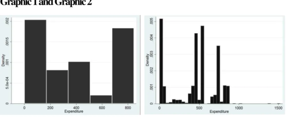
Relative distributional methods consist of non-parametric statistical processes. Nonparametric density estimates

allow for the comparison between groups and to a group with a benchmark density (e.g. the normal).16 It does not require the adoption of assumptions in what concerns the mathematical form of the probabilities distribution of a variable.17 Hence, non-parametric models prevent violations of the hypothesis of models

which would lead to misleading answers. The two histograms below, showing the expenditure level of two specific medical physicians, highlight how hard it would be to find a benchmark density suitable for every

medical physician regarding his/her number of prescriptions over prices/value per prescription:

Graphic 1 and Graphic 2

14

Further information can be found in the Extra Annexes, section A.1. 15

According to Barnett and Lewis (1994) an outlier is: “An observation (or subset of observations) which appears to be inconsistent

with the remainder of that set of data.”

16

Cameron et al. (2005) 17

(8)

8 Moreover, it contains a graphical component, which simplifies the analysis.

This method establishes an association among distributions, allowing the possibility of making direct

comparisons between groups or points in time, with respect to a continuous outcome variable. A reference group must be set, as well as a comparison group. Comparisons are done by getting comparison group’s points and understand where they fall in the reference distribution (i.e. in which quantile). Thus, it converts two

distributions into a single one allowing for an analysis that is scale independent (it shows the set of percentage positions that the observations of one distribution would have were they located in another distribution). If both distributions are equal, then the “relative data” will be uniformly distributed.

As stated by Handcock e Morris (1999), relative distribution methods include particularities such as not being affected by the scale choice or to monotonic transformations, basing its study in the population and not the

individual and it computes proportions of individuals and calculates their ranking position.

Let Y0 be theoutcome variable in the reference group, and Y be the outcome variable in the comparison group. It is usually the measurement for a different group or it can be the identical group in another time period.

Being F0 the distribution function of the reference group we have that R= F0 (Y)

The Cumulative Distribution Function (CDF) of the relative data R is given by:

G(r) = F [F0-1 (r)] = Q0 (r)0≤r≤1 where Q0 (r) is the quantile function of the reference distribution Taking the first order derivative of G(r) the density function is obtained:

g(r) = f{[F0-1 (r)]} / f0{[F0-1 (r)]} = f [Q0 (r)]/ f0[Q0 (r)] 0≤r≤1 where f and f0 are density functions The relative distribution allows to directly compare one distribution with another.

It is expressed as a random variable which was attained by converting a variable from the comparison group

(9)

9 The Probability Density Function (PDF) may be interpreted as a density ratio between two different

distributions i.e., “the ratio of the fraction of respondents in the comparison group to the fraction in the reference group at a given level of the outcome attribute”. To use the relative distribution model one only needs to

include those that have prescribed at least more than four times.

To complement the visual component, the Kolmogorov-Smirnov test is used to test the hypothesis whether two samples follow the same distribution or not.18 Specifically, it will be compared the distribution of the

expenditure level of each physician with the expenditure level of the other physicians excluding himself/herself. The null hypothesis assumes that the samples are drawn from the same distribution. This test requires

continuous distributions, as in this case, and it is a non-parametric method. Therefore, such analytical components are appropriate to use in this analysis.

3.2.1 Stochastic Dominance

To compare the evolution of each physician’s expenditure across time the stochastic dominance analysis is

applied. Stochastic dominance approaches have been traditionally applied in economics in relation to assets with monetary payoffs and in relation to poverty and income distribution analysis.19

The several types of pharmaceutical drugs used in each type of medical treatment entail an expenditure distribution. In this case, the First Stochastic Dominance (FSD) will be useful to compare expenditure levels,

between two periods, for each doctor. Therefore, applying a stochastic dominance technique offers the opportunity to identify whether expenditure levels for a given physician have been rising or falling across time. However, one has to consider that a physician’s expenditure level in pharmaceuticals is also affected by price

effects. A specific case is a modification in law that may contribute to changes in pharmaceutical expenditures across time. Indeed, since the 1st of March of 2013, the reference prices for pharmaceutical products changed.20

The assumption is that both, the physicians’ and patients’ characteristics, remain constant across time.

3.2.1.1 First-degree stochastic dominance (FSD)

18

Further information can be found in the Extra Annexes, section B.1. 19

Madden (2009) 20

(10)

10 Suppose that there are two possible distributions F and G, with cumulative density functions (CDF) of F(x)=Pr(X≤x) and G(x)=Pr(X≤x).

The CDF of F(x) dominates G(x) by first degree stochastic dominance if and only if: F(x)≤G(x), for all x

3.2.3. Ordered probit model

An ordered probit model is implemented to assess which characteristics associated with the outlier physicians are significant in explaining their expenditure levels’ deviation to the norm. This model was not run for

rheumatism since there are too few observations. The dependent variable, being an outlier (y) is a limited dependent variable which takes the following form: y=1 if the physician is an outlier with an expenditure level above the norm and y=-1 if the physician is an outlier with an expenditure level below the norm and y=0 his

expenditure is according to the norm.

-1 if the physician is an outlier with an expenditure level below the norm Y = 0 his expenditure is according to the norm

1 if the physician is an outlier with an expenditure level above the norm

Being yi* = xi’β + ui a latent index model where yi = (-1,0,1) For a three alternative ordered probit model: yi =-1 if yi*≤ α1

yi=0 if α1< yi*≤ α2 yi=1 if yi*≥ α2

Thresholds separate the ordering of alternatives. In this case we have:

Pr(yi =-1) = Pr(yi ≤ α1) = Pr(xi β +εi≤ α1) = Pr(εi≤ α1- xi β) = Φ[α1- xi β] = 1- Φ[xi β–α1]

Pr(yi=0) = Pr(α1 < yi* ≤ α2) = Pr(yi* ≤ α2) – Pr(yi* ≤ α1)= Pr(xi β +εi≤ α2) – Pr(xi β +εi≤ α1) = Pr(εi≤ α2- xi β) -

Pr(εi≤ α1 - xi β) = Φ[α2- xi β] - Φ[α1- xi β] = 1 - Φ[xi β–α2] – 1 + Φ[xi β - α1] = Φ[xi β - α1] - Φ[xi β–α2] Pr(yi=1) = Pr(yi* > α2) = Pr(xi β +εi> α2) = Pr(εi> α2- xi β) = 1 - Φ[α2- xi β] = Φ[xi β–α2]

(11)

11 It would be desirable to include other characteristics of the physicians such as sex, age and education level.

Unfortunately such information was not available. Unordered multinomial models could also be used, but to take into account the ordering makes this model more parsimonious. P is the probability of the outcome.

To ensure that 0 ≤ p ≤ 1 it is natural to specify F(·) to be a cumulative distribution function.21

In the case of the

probit, this cumulative distribution function will be the standard normal one. The explanatory variables are the current hospital where the physician works, the number of prescriptions prescribed by him/her and his/her medical specialty. The aim is to understand which factors influence physicians’ prescribing patterns. Given the

small number of observations in what concerns rheumatism, the model will only focus on HIV and oncology pharmaceutical products’ prescriptions. Since the ordered probit is constructed based on the results attained by

the relative distribution, all physicians prescribing less than four times were excluded.

4. Results 4.1. HIV

4.1.1. Comparisons among physicians

This database includes 176 physicians prescribing HIV-related pharmaceutical products. However, only those prescribing more than four times were included in this analysis. Each physician’s expenditure was compared with his colleagues’ expenditure. Afterwards each graph was analysed as to conclude about the physician’s

expenditure: physicians incurring into higher or lower expenditure levels than the norm, in comparison to their colleagues. HSJ, HSAC and HCC are the hospitals whose specialty is HIV cases and therefore, register a

higher number of cases and a higher overall expenditure. Analysing a specific physician as an example:

Probability density function Cumulative density function

21

(12)

12 By looking at the probability density function, one sees that this physician shows a big discrepancy compared

to his colleagues from around the 38th to the 70th percentile, showing a higher expenditure, on average, than his colleagues. However, from the 0th to the 37th and from the 70th percentile on, it shows, on average, a lower

expenditure than his colleagues. This means that this physician in particular prescribes a higher quantity of less expensive pharmaceutical drugs than his colleagues, but also a higher quantity of more expensive pharmaceutical products.

By looking at all the computed graphs, it was notorious that there are many different patterns of prescription thus, it is not possible to establish a typology. Following the visual analysis of the graphs obtained in the relative

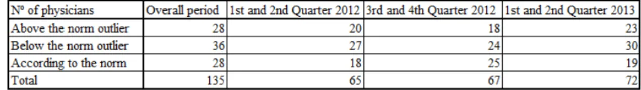
distribution and the Kolmogorov-Smirnov test, physicians were separated in three different groups. Let -1 represent physicians incurring into lower expenditure levels than the norm, in comparison to their colleagues, 0 represent those prescribing values according to the norm, and 1 represent those incurring into higher

expenditure levels.

Table 2 – Relative distribution results after the Kolmogorov-Smirnov test

Considering this, histograms were computed, taking into account that data is discrete and that the each class width is one, and therefore the density equals the relative frequency (since the density is the quotient of the

relative distribution with the class width). Seeing the overall period of analysis (six quarters), the histogram below shows the density of the physicians’ expenditure levels. One can conclude that the class with the highest

(13)

13

Graphic 5

Overall period

Analysing semester by semester, one can see that the densities among each class in the first semester of 2012 and in the first semester of 2013 look a-like, although in the latter one there is a higher density of physicians

with an above the norm expenditure level.

Graphic 6, Graphic 7 and Graphic 8

2012 1st_{and 2}nd_{Quarters; 2012 3}rd_{and 4}th_{Quarters; 2013 1}st_{and 2}nd_Quarters

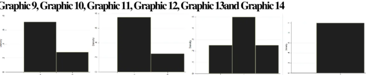
To analyse prescription patterns per hospital where each physician was prescribing, in the overall period, histograms were computed. However, one should note that in each quarter, the average, which is the reference

point, changes. In MAC and the density of physicians that are outliers prescribing below the average’s norm, in comparison to their colleagues is the greatest. Those prescribing in both HSAC and HSJ, have the same

quantity of physicians prescribing on the norm and above it. One should also highlight that those prescribing in HSJ, HCC and HSAC; HSJ, HDE and in HSJ, HSM were never outliers, when considering the overall period).22 It should be highlighted that in the specific case of HSJ, physicians dealing with HIV cases gather

and make prescribing decisions together.23 Across the three semesters, this hospital shows great density of physicians incurring into expenditure levels below the norm, in comparison to their colleagues (0,6; 0,4 and 0,6

respectively). Thus, there is a great variation in prescribing patterns across hospitals.

22

More details are available in the extra annexes, in the C.1.2. section 23

(14)

14

Graphic 9, Graphic 10, Graphic 11, Graphic 12, Graphic 13and Graphic 14

Alfredo da Costa; Santa Marta; Capuchos, S. José, while the last histograma refers to both São José, Curry e Cabral, Capuchos; São José, Estefânia and São José, Santa Marta Histograms across medical specialties were also computed.

Dermatovenereology; Endocrinology; Anesthesiology, Internal Physician, Clinical Pathology and Urology

In what concerns the medical specialty of the physicians prescribing HIV related pharmaceutical products, the assumption is that the “type” of patients is not related to the specialty of the physician. Considering the “extreme” cases24

, specialists in Dermatovenereology were only outliers below the norm, Endocrinology

always above and Anesthesiology, Internal Physician, Clinical Pathology and Urology were always

prescribing according to the norm.25

4.1.2. Outlier physicians across semesters

It is important to assess whether physicians are always showing the same outlier prescribing patterns in the period of analysis or if there is any change. For this purpose, the histograms below were computed for

physicians with according to the norm, above the norm and below the norm expenditure levels.

In what concerns physicians identified as outliers because they incurred into higher expenditure levels, half of them were outliers only during one period. The other half was showing this behaviour throughout three

24

Hospitals which only registered outliers that incur into expenditure levels above or below the norm 25

(15)

15 semesters (27%) and two semesters (23%). Thus, approximately half of the physicians considered outliers

incurring into higher expenditure levels than the norm tend to maintain their prescribing patterns across the period of observation.

Regarding physicians considered outliers with lower expenditure levels than the norm, the majority was showing this behaviour during two semesters, followed by those displaying this behaviour one semester.

4.1.3. Expenditure levels across semesters

A stochastic dominance approach was used to compare each physician’s expenditure level between two

different periods. Consecutive quarters were analysed and compared, throughout a graphical analysis. The graph below illustrates this approach:

Graphic 17

Stochastic Dominance Function

This figure represents a particular medical physician and his/her expenditure levels in the 1st quarter of 2012 and on the 2nd quarter of 2012. One can see that the distribution of the 2nd quarter of 2012 is everywhere above the

distribution of the 1st quarter of 2012. Therefore, the distribution of the 1st quarter of 2012 first order stochastically dominates the one of the 2nd quarter of 2012. Assuming that the benefits are the same, lower expenditure levels are considered better. Therefore, in this specific case, expenditure with pharmaceutical

products increased from one quarter to the other and the distribution developed in a undesired way.

Being Dit = 1 if t stochastically dominates t-1 (the expenditure level in t is lower than in t-1) and Dit = 0 if t-1

(16)

16

Graphic 18, Graphic 19, Graphic 20, Graphic 21 and Graphic 22

For the majority of the physicians prescribing HIV related pharmaceutical products in the first semester of

2012, the distribution of the 1st quarter of 2012 first order stochastically dominates the one of the 2nd quarter of 2012. The expenditure level of HIV related pharmaceutical products has, therefore, increased from the 1st to

the 2nd quarter of 2012 for more than a half of medical physicians. From the 2nd to the 3rd quarter of 2012, approximately more than a half of medical physicians increased their expenditure levels in pharmaceuticals. The same pattern occurs from the 3rd to the 4th quarter of 2012 and well as for the 1st to the second quarter of

2013. The period from the 4th quarter of 2012 to the 1st quarter of 2013 was an exception, in the sense that there were more physicians incurring into lower expenditure levels in the latter period (the 1st quarter of 2013). Such

event may be related to the fact that since August (3rd quarter of 2012) physicians started to receive feedback about their and the total expenditure level in pharmaceuticals. It may also have to do with the fact that, since the 1st of March of 2013, the reference prices for pharmaceutical products changed.26 The newly selected countries were chosen based on their lower pharmaceutical products’ price.27The 1st semester of 2013 is the one that

shows a higher discrepancy between the two quarters, with the majority of physicians incurring into higher

expenditure levels in the 2nd quarter. Thus, one can conclude that expenditure levels have been increasing over

26

Ordinance n.º 91/2013 27

According to the Ordinance n.º 91/2013: “Atendendo à necessidade de racionalização dos encargos públicos com medicamentos,

(17)

17 time for most physicians, except in one period. However, it is not possible to assess if this change was due to

the number of treated patients since only after 2013 all the hospitals were using the same database. Thus, different patients from different hospitals may, in 2012, have the same patient number. Nevertheless, one can

look at the quantity and unit price of the pharmaceuticals prescribed. In what concerns the unit price, there is an increase in the prescription of very costly pharmaceutical products since the first two quarters of 2012 (although they represent really small densities). In what concerns the quantity, it seems that there are no major changes

across time.28

2012 1st_-2nd_{Quarter 2012 2}nd_-3rd_Quarter

4.1.4. Significant Characteristics

The explanatory variables include the number of prescriptions made by each physician, the medical specialty (a dummy variable with 1 being Infectiology and General Medicine and 0 the other specialties, since these are

the two specialties which physicians register a larger number of episodes) and the hospital where he/she prescribes (dummy variables, being the omitted variable HSM). As it was previously stated in the data description, it is not possible to follow a patient by his/her hospital number. Neither patients’nor physicians’

characteristics (e.g. age, education and job) are available. It might be possible that some of these variables could be significant into explaining different expenditure levels.

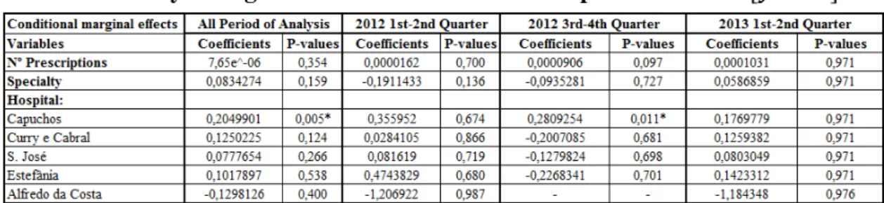
Table 3 – Ordered probit results

28

(18)

18 Prescribing in HSAC is significant in the overall period of analysis and in two semesters, associated with positive coefficients. The medical specialty of the physician prescribing is significant in the 1st semester of 2012.

In the unordered probit case, the sign of each coefficient gives the direction of the effect, but not its marginal

effect.29 The marginal effects of changes in the explanatory variables are given by:

{F(αj-1-xiβ) -

F(αj-xiβ)}β.30

Table 4 – Probability of being an outlier with a below the norm expenditure level - P

Table 5 - Probability having an expenditure level according to the norm -

Table 6 – Probability of being an outlier with an above the norm expenditure level - P

29

For further details see section B.1. of the Extra Annexes 30

(19)

19 The main result is that physicians prescribing in HSAC are more likely to be outliers incurring into

expenditures above the norm (20 percentage points in the overall period and 28 percentage points in the 2nd semester of 2012) and less likely to be outliers incurring into expenditures below the norm (25 percentage

points in the overall period and 34 percentage points in the 2nd semester of 2012), in comparison to those prescribing in HSM (the omitted variable).

4.2. Oncology

This dataset contains 193 physicians prescribing oncology related pharmaceutical drugs. However, to use the

relative distribution model one needs to only include those that have prescribed at least more than four times, therefore only 135 physicians were analysed.

The density of outliers incurring into higher expenditure levels than the average seems to be more or less

constant across the three semesters.

HSJ shows a decrease in outlier physicians prescribing levels above the norm throughout the three semesters. HSAC consistently has a great density of outlier physicians prescribing below the norm expenditure level. On

the other hand, HCC displays great density outlier physicians prescribing levels above the norm throughout the three semesters.31

There is also great divergence between medical specialties.32 Considering the overall period, there are six specialties which physicians are all outliers prescribing above the norm level and one where they are not outliers. However, in what concerns cancer, different medical specialties are related to several types of cancer.33

Different types of cancer require different a treatment so, costs are not comparable across the different pathologies.

31

(20)

20 In what concerns physicians identified as outliers because they have incurred into higher expenditure levels, on

average, than their colleagues, most of them were showing this behaviour throughout the three semesters. By analysing the physicians that were identified as outliers that incurred into lower expenditure levels, than their

colleagues, the majority also showed this pattern during the three semesters. Thus, most physicians have been maintaining their prescribing patterns unchanged.34

The expenditure level of oncology related pharmaceutical products has increased from the 1st to the 2nd quarter of 2012, from the second to the third quarter of 2012 and from the 4th quarter of 2012 to the 1st quarter of 2013 .

On the other hand, from the 3rd to the 4th quarter of 2012 and from the 1st to the 2nd quarter of 2013 there is a greater density for physicians incurring into lower expenditure levels in the latter period. This might be related to the fact that since August (in the 3rd quarter of 2012) physicians started to have feedback about their and the

total expenditure level in pharmaceuticals Furthermore, since the 1st of March of 2013,the reference prices for pharmaceutical products changed. The newly selected countries were chosen based on their lower pharmaceutical products’ price. With respect to the quantity and the unit price of the pharmaceutical products

prescribed, there are no major changes across these 1,5years. In some periods, there is a small density of pharmaceutical products which unit price is extremely high (more than 1000€), which may be related to very

acute episodes.

4.2.4. Significant Characteristics

In what concerns cancer, different medical specialties are related to several types of cancer, as it was stated

before. Across each semester and in the overall period the only significant variables are those concerning the physician’s medical specialty. However, one cannot do such comparison. In what concerns the number of

34

(21)

21 pharmaceutical products that were prescribed and the hospital where they were prescribed, no coefficient is

significant.35

4.3. Rheumatism

In what concerns physicians prescribing for rheumatology, they are concentrated in three out of the six hospitals: HCC, HSAC, and HDE. HCC seems to have more physicians incurring into higher expenditure

levels than the norm. This pattern is consistent throughout the different semesters. The opposite happens with HSAC and HDE, which have a higher proportion of physicians incurring into lower expenditure levels than

the norm.36

General Medicine is the medical specialty with more physicians with expenditure levels above the norm, when considering the overall period. In what concerns the specialty of the medical physicians below the norm

, the results show that the majority are specialists in Anesthesiology and Pediatrics. This is true both for the overall period and for each semester.37

Regarding physicians identified as outliers because they incurred into higher expenditure levels, on average, than their colleagues, the majority were showing this behaviour throughout two semesters followed by those

showing this behaviour during three semesters. There was no physician showing this pattern only in one semester.

By analysing the physicians that were identified as outliers that incurred into lower expenditure levels than their

colleagues, the majority showed this pattern during one semester, followed by those showing this behaviour during three semesters.

35

(22)

22 Expenditure levels in pharmaceuticals have been decreasing in 3 out of 5 periods (from the first to the 2nd

quarter of 2012, from the 2nd to the 3rd quarter of 2012 and from the 4th quarter of 2012 to the 1st quarter of 2013). Thus, expenditure levels have been decreasing over time for most physicians, except for two periods.

Regarding the unit price, there is an increase in the prescription of very costly pharmaceutical products since the first two quarters of 2012. In what concerns the quantity, it seems that there are no major changes across time.38

5. Conclusion

Regarding HIV, there is a great variation in prescribing patterns across hospitals. One should highlight the case of HSJ, where physicians dealing with HIV cases gather and make prescribing decisions together. During the

observation period, this hospital shows a high density of physicians incurring into expenditure levels below the norm, in comparison to their colleagues. Concerning the permanence/change of the prescribing behaviour by physicians, it was found that approximately half of the physicians that were considered as outliers, incurring

into higher expenditure levels than the norm tend to maintain their prescribing patterns across these 1,5 years. Expenditure levels in pharmaceutical products have been increasing over time for most physicians, except in one period. With respect to the unit price, there is an increase in the prescription of very costly pharmaceutical

products since the first two quarters of 2012, however the quantity prescribed did not register major changes across time. The unordered probit model consistently shows that physicians prescribing in HSAC have a

higher probability of being outliers incurring into higher expenditures than the norm and a lower probability of being outliers incurring into lower expenditure levels than the norm, in comparison to those prescribing in HSM (the omitted variable).

Physicians prescribing oncology-related pharmaceutical products seem to have very different prescription patterns according to the hospital where they prescribe. HSJ shows a decrease in outlier physicians prescribing

levels above the norm throughout the three semesters. HSAC consistently has a great density of outlier physicians prescribing below the norm expenditure level. HCC displays a great density of outlier physicians

38

(23)

23 prescribing levels above the norm throughout the three semesters. Regardless of the hospital, most physicians

have been maintaining their prescribing patterns unchanged. There are also great differences across medical specialties. However, different types of cancer require different treatments and thus,, costs are not comparable

across different pathologies. As to the stability of outlier behaviour, most physicians have not been changing their prescribing patterns. With respect to the quantity and the unit price of the pharmaceutical products prescribed, there are no major changes across the observation period. In some periods, pharmaceutical products with a extremely high unit price (more than €1.000, while almost all the others cost less than €500) are

prescribed. However, they only represent a small density of the overall products. This may be related to very

acute episodes, which require costlier products.

In what concerns rheumatism, physicians are concentrated in three out of the six hospitals: HCC, HSAC, and HDE. HCC seems to have more physicians incurring into higher expenditure levels than the norm. This

pattern is consistent throughout the different semesters. The opposite happens with HSAC and HDE, which have a higher proportion of physicians incurring into lower expenditure levels than the norm. Most of outlier physicians that incur in higher expenditures maintain their prescribing behaviour throughout this period. In

contrast, those that incur in lower expenditure levels than the norm do not maintain their prescribing behaviour. Expenditure levels have been decreasing over time for most physicians, except for two periods. Regarding the

unit price, there is an increase in the prescription of very costly pharmaceutical products since the first two quarters of 2012. In what concerns the quantity, it seems that there are no major changes across time.

Overall, there is great divergence of prescribing patterns across physicians, the hospitals where they prescribe

and their medical specialties. Physicians tended to maintain their prescribing patterns across these 1,5 years, whether they were outliers incurring into higher or lower expenditure levels than the norm and even after the

(24)

24 The results stated above show a discrepancy in relation to the Law of Large Numbers. This law states that, on

average, each physician should treat similar patients, in terms of health status and related expenditure. Hence, it should be expected that prescription patterns of pharmaceuticals would be similar across hospitals and across

physicians with the same medical specialty. Therefore, there is room to reduce hospital costs of pharmaceutical products, by better practice of physicians.

Nevertheless, it would be valuable to have information regarding the treated patients. Then one could assess

whether physicians that are always incurring into expenditure levels above the norm were treating patients that could justify the use of costlier pharmaceutical products or not (since in some cases the application of the Law

of Large Numbers might be unsuitable). If it would be found that such patients did not require costlier pharmaceutical products, then one could conclude that these physicians should change their prescribing behaviour while the other ones (incurring into below the norm expenditure levels) should be emphasised as

having a better practice.

Future research should include a method, such as the differences-in-differences one, to evaluate whether physicians change their prescription patterns when they are provided with better information regarding their

prescription behaviour. Furthermore, in the specific case of HIV, it would be interesting to assess the impact of physicians prescribing pharmaceutical products together, by analysing the case of HSJ. 39 Moreover, having

information about the patients’ as well as physicians’ characteristics (e.g. sex, age and education level.) could be beneficial for further research.

6. Bibliography

Allan, GM; Lexchin, J and Wiebe, N. 2007. “Physician Awareness of Drug Cost: A Systematic Review”. PLoS Med 4(9): e283. 3edition

Araújo, A., Barata; F., Barroso, S., Cortes, P., Damasceno, M., Parreira, A., Espírito Santo, J., Encarnação Teixeira and R. Pereira. 2009. “Custo do Tratamento do Cancro emPortugal”.

Atkinson, Anthony B. 1970. “On the measurement of inequality”, Journal of Economic Theory, 2:244-263.

Barnett, V and T. Lewis.1994. Outliers in Statistical Data. John Wiley & Sons.,

Bradley C. 1991. “Decision making and prescribing patterns –a literature review”. Family Practice 8, 276-87.

Bradley, C.1995. “Prescription Decisions in General Practice–Learning and Changing” Occasional Paper of the Royal College of General Practice, Chpater 3: 10-12.

39

(25)

25

Bruce C. Stuart, Jalpa A. Doshi, and Joseph V. Terza. 2009. “Assessing the Impact of Drug Use on Hospital Costs”. Health Services Research, vol. 44, no. 1, pp. 128–144.

Cameron, A.C. and P.K. Triverdi. 2005. Microeconometrics: methods and applications. New York, USA: Cambridge University Press.

Carone, Giuseppe & Schwierz, Christoph and Ana Xavier. 2012. "Cost-containment policies in public pharmaceutical spending in the EU," MPRA Paper 42008, University Library of Munich, Germany.

Chew LD, O'Young TS, Hazlet TK, Bradley KA, Maynard C and DS. Lessler.2000. “A physician

survey of the effect of drug sample availability on physicians' behavior”.J Gen Intern Med 2000;15: 478-483.

Culver, A. J. and J. P. Newhouse .2000. Handbook of health economics. Amsterdam; New York: Elsevier

Diário da República Eletrónico http://tinyurl.com/ppw2lml (accessed 1st December 2013)

E. Wolfstetter. 1996. “Stochastic Dominance: Theorie and Applications”. SFB 373 Discussion Papers

1996,40, Humboldt University of Berlin, Interdisciplinary Project 373: Quantification and Simulation of Economic Processes.

Eurobarometer http://tinyurl.com/4c5qsk (accessed 22nd June 2013).

European Commission http://tinyurl.com/lgr7p9b (accessed 22nd June 2013).

Gartner. 2009. “eHealth for a Healthier Europe!”, Ministry of Health and Social Affairs in Sweden.

Handcock, Mark S., and Martina Morris.1998. “Relative Distribution Methods. Sociological Methodology 28: 53-97.

Hart, J., Salman, H., Bergman, M., Neuman, V., Rudniki, C., Gilnenberg, D., Matalon, A. and M. Djaldetti. 1997. “Do drug costs affect physicians' prescription decisions?”. Journal of Internal Medicine, 241: 415–420.

Heffler, S., S. Smith, S. Keehan, C. Borger, M. Clemens, and C. Truffer. 2005. ‘‘U.S. Health Spending Projections for 2004–2114.’’ Health Affairs 24 (suppl): W5–W74 (February).

Hogerzeil HV.1995.“Promoting rational prescribing: an international perspective”. Br. J. Clin. Pharmacol.,39: 1-6.

Schroeder SA, Myers LP, McPhee SJ, Showstack JA, Simborg DW, Chapman SA and JK. Leong. 1984. “The failure of physician education as a cost containment strategy. Report of a prospective controlled trial at a university hospital”. JAMA : the Journal of the American Medical Association 252(2):225-230.

IMF.2013. “Portugal – Memorandum of Understanding on specific economic policy conditionality, 5th update”. http://tinyurl.com/c7foww5 (accessed 22nd June 2013).

Lucas, Raquel. 2012. “Os custos das doenças reumáticas e os ganhos com a sua terapêutica adequada (uma

perspectiva epidemiológica) ”. Fórum de Apoio ao Doente Reumático.

Madden, David. 2009. Mental stress in Ireland, 1994-2000: a stochastic dominance approach. Health Economics 18:10, 1202-1217.

Perelman, J.; Alves J.;. Mateus, C; Pereira, J.; Mansinho, K.; Miranda, A.; Antunes, F.; Doroana, M.; Oliveira, J.; Poças, J.; Marques, R. and E. Teófilo. 2011. “Direct Treatment Costs for HIV/AIDS in Portugal”. Conferência Nacional de Economia da Saúde .

Virji, A. and N. Britten.1991. “A study of the relationship between patients’ attitudes and doctors’ prescribing”. Family Practice, 8, 314–319.

Wolfstetter, Elmar. 1999. Topics in Microeconomics, Cambridge: Cambridge University Press.

World Health Organization. 1995. Guide to Good Prescribing. Geneva, World Health Organization. World Health Organization. 2010. The world health report 2010: Health Systems Financing: the Path to Universal Coverage Geneva, Switzerland: World Health Organization.

(26)

26

Extra Annexes

Prescription Patterns of Pharmaceuticals

Ana Sofia Oliveira Gonçalves #543

(27)

27

Annex A

A.1. Database Description

(28)

28

B – Detailed Methodology

B.1. Kolmogorov-Smirnov Test

The two-sample Kolmogorov-Smirnov test (Dn) is used to assess whether or not two

samples follow the same distribution, by comparing each cumulative distribution function.

Taking F(x) and G(x) as empirical distribution functions for the sample being compared, the hypotheses being tested are:

D+=maxx {F(x) – G(x)}

D-= minx {F(x) – G(x)}

The combined statistical test is therefore given by: D=max (|D+| , |D-|)

As an example:

Smaller group D P-value Corrected --- 0: 0.1168 0.682

1: -0.5206 0.001

Combined K-S: 0.5206 0.001 0.000

The first line tests the hypothesis that the Expenditure for group 0 (every physician

excluding the one being analysed) contains smaller values than for group 1 (the physician being analysed). Since the p-value is 0,682, it is not significant and thus we

cannot reject the null hypothesis.

The second line tests the hypothesis that the Expenditure for group 0 contains larger values than for group 1. The p-value is 0,001, which is significant. Thus, the null

hypothesis is rejected.

(29)

29

When the dependent variable has a finite number of possible outcomes, the data is called multinomial. In this case, the dependent variable chosen assumes three different

values. The dependent variable not only assumes three different values, but is also ordinal in the sense that it assumes that there is a latent continuous metric underlying

the ordinal responses observed by the analyst.

-1 if the physician is an outlier with an expenditure level below the average

Y = 0 his expenditure is according to the norm

1 if the physician is an outlier with an expenditure level above the average

Therefore binary response models are not suitable for this analysis, since in these

models the dependent variable can only assume two different values.

In what concerns the choice between an ordered probit or an ordered logit, Heij et al.

(2004) state that “there are often no compelling reasons to choose between the logit and

probit model”.

Being yi* = xi’β + ui a latent index model where yi = (-1,0,1) For a three alternative

ordered probit model: yi =-1 if yi* ≤ α1

yi=0 if α1< yi*≤ α2

yi=1 if yi*≥ α2

Thresholds separate the ordering of alternatives. In this case we have:

Pr(yi =-1) = Pr(yi ≤ α1) = Pr(xi β +εi ≤ α1) = Pr(εi ≤ α1- xi β) = Φ[α1- xi β] = 1- Φ[xi β–α1]

Pr(yi=0) = Pr(α1 < yi* ≤ α2) = Pr(yi* ≤ α2) – Pr(yi* ≤ α1)= Pr(xi β +εi ≤ α2) – Pr(xi β +εi ≤ α1) =

Pr(εi ≤ α2- xi β) - Pr(εi ≤ α1 - xi β) = Φ[α2- xi β] - Φ[α1- xi β] = 1 - Φ[xi β–α2] – 1 + Φ[xi β - α1] =

Φ[xi β - α1] - Φ[xi β–α2]

Pr(yi=1) = Pr(yi* > α2) = Pr(xi β +εi > α2) = Pr(εi > α2- xi β) = 1 - Φ[α2- xi β] = Φ[xi β–α2]

(30)

30

The sign of the regression parameters β gives the direction of the effect i.e., whether or

not the latent variable y* increases or decreases with a change in the regressor.

However, it gives no information regarding the sign of the marginal effect. The marginal effects of changes in the explanatory variables are given by:

{F(αj-1-xiβ) - F(αj-xiβ)}β

Marginal effects can be used with categorical variables, which are included in this ordered probit.

B.3.Differences-in-Differences

To assess whether or not making physicians aware of their expenditure levels in pharmaceutical products a Differences-in-Differences (DD) method could be used.

The DD method provides a tool to estimate causal effects when using panel data that contains groups of observations which are exposed and not exposed to a causing

variable.

The treatment, an exogenous event, would only affect a set of individuals, the treated individuals. Physicians in these six hospitals are given feedback about their expenditure

levels in pharmaceuticals, as well as hospitals’ total expenditure in these products. This

feedback is available since August 2012 and physicians can check it by logging in their

personal intranet page. However, some physicians may regularly control this information, while others may not even log in. Therefore, an interesting treatment, would be to do a survey to some physicians that, indirectly, would make them be aware

of that feedback. Furthermore, in the specific case of HIV, it would be interesting to assess the impact of physicians prescribing pharmaceutical products together, by analysing the case of HSJ in comparison to the

other five hospitals.

Assuming two time periods, where treatment occurs only in period 2:

(31)

31

Di2=0 – untreated individuals in period 2

Di2=1 – treated individuals in period 2

∆yi= φ Di + δ + vi

Where δ is a fixed effect and D i a binary treatment variable, indicating if the individual

received, or not, treatment.

The resulting estimator is called DD estimator because it estimates the time difference for the treated and untreated groups, followed by taking the difference in the time

differences.1

Thus, this method is going to be used to measure the causal effect of the treatment on

expenditure levels and prescription patterns of pharmaceuticals.

(32)

32

C – Detailed Results C.1. – HIV

C.1.1.Kolmogorov-Smirnov Test results

Table 2 - Relative distribution results after the Kolmogorov-Smirnov test

C.1.2. Comparisons among physicians – per hospital(s) where each one prescribes

C.1.2.1. Overall period

Alfredo da Costa; Capuchos; Curry e Cabral

Estefânia; São José; Santa Marta

(33)

33

Curry e Cabral and São José; São José and Estefânia; São José and Santa Marta

C.1.2.2. 1st Semester of 2012

(34)

34

S. José and Curry e Cabral; S. José and Capuchos; S. José and Santa Marta

C.1.2.3. 2nd Semester of 2012

Capuchos; Curry e Cabral; Estefânia

S. José; Santa Marta

Curry e Cabral and S. José; Curry e Cabral and Capuchos and S. José; Capuchos and Curry e Cabral; Capuchos and S. José

C.1.2.4. 1st Semester of 2013

(35)

35

Curry e Cabral and S. José; Curry e Cabral and Capuchos; Curry e Cabral and S. José and Capuchos; Capuchos and S. José

Capuchos and S. José and Santa Marta; Estefânia and S. José; S. José and Santa Marta

C.1.3. Comparisons among physicians – per medical specialty C.1.3.1 Overall period

Anesthesiology; General Surgery; General and Family Practice; Dermatovenereology

(36)

36

Infectiology; Occupational Medicine; General Medicine; Resident Physician

Nephrology; Medical Oncology; Clinical Pathology; Medical Pediatrics; Urology

C.1.3.2. 1st Semester of 2012

General and Family Practice; Dermatovenereology; Gastroenterology; Gynecology & Obstetrics

Clinical Hematology; Infectiology; Occupational Medicine; General Medicine

Medical Pediatrics

C.1.3.3. 2nd Semester of 2012

Anesthesiology; General Surgery;Dermatovenereology; Gastroenterology

(37)

37

Pediatrics

C.1.3.4. 1st Semester of 2013

General Surgery; General and Family Practice; Dermatovenereology; Gastroenterology

Gynecology & Obstetrics; Infectiology; Occupational Medicine; General Medicine

Resident Pysician; Nephrology; Clinical Pathology

C.1.4. Expenditure levels across semesters C.1.4.1. Quantity and Unit Price

(38)

38

2012 2nd_-3rd_Quarter

2012 3rd_{- 4}th_Quarter

2012 4th_{– 2013 1}st_Quarter

(39)

39

C.2.5. Ordered probit results

Table 3 – Ordered probit coefficients and p-values

Table 4 - Probability of being an outlier with a below the norm expenditure level - P

C.2. – Oncology

C.2.1. Kolmogorov-Smirnov Test results

(40)

40

C.2.2.1. Overall Period

S. José; Estefânia; Santa Marta

Alfredo da Costa and Estefânia; Curry e Cabral and Alfredo da Costa; Curry e Cabral and S. José; Capuchos and Alfredo da Costa

Capuchos and S. José; S. José and Alfredo da Costa and Capuchos; S. José and Alfredo da Costa

C.2.2.2. 1st Semester of 2012

(41)

41

Estefânia; S. José

Alfredo da Costa and Capuchos; Alfredo da Costa and Capuchos and S. José; Alfredo da Costa and S. José; Capuchos and S. José

S. José and Curry e Cabral

C.2.2.3. 2nd Semester of 2012

Capuchos; Curry e Cabral; Estefânia; S. José

(42)

42

S. José and Curry e Cabral

C.2.2.4. 1st Semester of 2013

Alfredo da Costa; Capuchos; Curry Cabral

S. José; Estefânia; Santa Marta

Alfredo da Costa and Capuchos; Alfredo da Costa and Capuchos and S. José; Alfredo da Costa and Estefânia; Alfredo da Costa and S.José

Curry e Cabral and S. José; Capuchos and S. José

C.2.3. Comparisons among physicians – per medical specialty

C.2.3.1 Overall period

(43)

43

Gastroenterology; Gynecology & Obstetrics; Clinical Hematology; Infectiology

General Medicine; Medical Oncology; Pediatrics; Pneumology

Urology

C.2.3.2. 1st Semester of 2012

Anesthesiology; General Surgery; Dermatovereology; Endocrineology

(44)

44

Urology

C.2.3.3. 2nd Semester of 2012

Anesthesiology; General Surgery; Dermatovereology; Gynecology & Obstetrics

Clinical Hemathology; General Medicine; Medical Oncology

Urology

C.2.3.4. 1st Semester of 2013

Anesthesiology; General Surgery; Dermatovereology; Gastroenterology

(45)

45

Medical Oncology; Pediatrics; Pneumology; Urology

2012 1st_-2nd_Quarter

2012 2nd_-3rd_Quarter

(46)

46

2012 4th_{- 2013 1}st_Quarter

C.2.5. Ordered probit results

Table 8 – Ordered probit coefficients and p-values

(47)

47

C.3. – Reumathism

(48)

48

C.3.2. Comparisons among physicians – per hospital(s) where each one prescribes

C.3.2.1. Overall Period

C.3.2.2. 1st Semester of 2012

C.3.2.2. 2nd Semester of 2012

(49)

49

C.3.3. Comparisons among physicians – per medical specialty

C.3.3.1. Overall period

Anesthesiology; Dermatovereology; General Medicine; Pediatrics

C.3.3.2. 1st Semester of 2012

Dermatovereology; General Medicine; Pediatrics

C.3.3.3. 2nd Semester of 2012

Anesthesiology; Dermatovereology; General Medicine; Pediatrics

(50)

50

Dermatovereology; General Medicine; Pediatrics

(51)

51

2012 3rd_{- 4}th_Quarter

2012 4th_{– 2013 1}st_Quarter

D. Detailed diseases’ description

D.1. HIV

Pharmaceutical products for HIV/AIDS related diseases are fully paid by the Portuguese

National Health System (PNHS) since 1996.2 3The PNHS takes the responsibility to

offer healthcare in all the disease stages of a person that is HIV-positive. Indeed, it was

in 1996 that an important treatment was introduced: the antiretroviral treatment. This treatment consists of combining at least three antiretroviral drugs, as a way to supress

the virus and limit its progression.4 Therefore, this disease started to be considered as

chronic, associated with a decrease in mortality and morbidity, allowing patients to be in the labour market.

(52)

52

Since the 1st of December 2012, all hospitals belonging to the PNHS are required to use

the SI.VIDA system.5 This system was created with the aim of monitoring the National

Program for HIV/SIDA Infection. Its main objective is to register every activity related to the supply of HIV/AIDS related healthcare, which means that every prescription has

to be done electronically. Prescriptions have to be done by physicians which are specialists in HIV, which can include physicians whose medical specialty is

Infectiology or General Medicine.6

D.2. Oncology

The Directorate-General of Health is currently elaborating clinical guidelines for the

different types of cancer as a way to improve medical practice.

The payment for oncology treatments assumes a treatment that lasts 25 months and distinguishes three different types: breast cancer, uterine cancer and colorectal cancer.

However, this payment procedure is still only applied to some hospitals, not including the ones belonging to the Centro Hospitalar de Lisboa Central. Therefore, it is assumed

that different types of cancer require different a treatment so, costs are not comparable

across the different pathologies.7

Table 13 – Costs of cancer by type per patient/month

5_{Decree Law nº 6716/2012}

6

Decree Law n.º 280/96

(53)

53

Bibliography

Administração Central do Sistema de Saúde (ACSS). 2012. “Contrato-Programa

2013”. Lisboa http://tinyurl.com/kqvk8nk (accessed 1st December 2013)

Cameron, A.C. and P.K. Triverdi. 2005. Microeconometrics: methods and