http://dx.doi.org/10.7494/OpMath.2015.35.3.293
FRAMES AND FACTORIZATION
OF GRAPH LAPLACIANS
Palle Jorgensen and Feng Tian
Communicated by P.A. Cojuhari
Abstract.Using functions from electrical networks (graphs with resistors assigned to edges), we prove existence (with explicit formulas) of a canonical Parseval frame in the energy Hilbert spaceHEof a prescribed infinite (or finite) network. Outside degenerate cases, our Parseval
frame is not an orthonormal basis. We apply our frame to prove a number of explicit results: With our Parseval frame and related closable operators inHEwe characterize the Friedrichs
extension of the HE-graph Laplacian. We consider infinite connected network-graphsG= (V, E),V for vertices, andE for edges. To every conductance functioncon the edgesEofG, there is an associated pair(HE,∆)whereHE in an energy Hilbert space, and∆ (= ∆c) is the c-graph Laplacian; both depending on the choice of conductance function c. When a conductance function is given, there is a current-induced orientation on the set of edges and an associated natural Parseval frame inHE consisting of dipoles. Now∆is a well-defined semibounded Hermitian operator in both of the Hilbert l2(V) and HE. It is known to
automatically be essentially selfadjoint as an l2(
V)-operator, but generally not as an HE
operator. Hence as an HE operator it has a Friedrichs extension. In this paper we offer
two results for the Friedrichs extension: a characterization and a factorization. The latter is vial2
(V).
Keywords: unbounded operators, deficiency-indices, Hilbert space, boundary values, weighted graph, reproducing kernel, Dirichlet form, graph Laplacian, resistance network, harmonic analysis, frame, Parseval frame, Friedrichs extension, reversible random walk, resistance distance, energy Hilbert space.
Mathematics Subject Classification: 47L60, 46N30, 46N50, 42C15, 65R10, 05C50, 05C75, 31C20, 46N20, 22E70, 31A15, 58J65, 81S25.
1. INTRODUCTION
We study infinite networks with the use of frames in Hilbert space. While our results apply to finite systems, we will concentrate on the infinite case because of its statistical significance.
c
By a network we mean a graph G with vertices V and edges E. We assume that each vertex is connected by single edges to a finite number of neighboring ver-tices, and that resistors are assigned to the edges. From this we define an associated graph-Laplacian∆, and a resistance metric onV.
The functions on V of interest represent voltage distributions. While there are a number of candidates for associated Hilbert spaces of functions on V, the one we choose here has its norm-square equal to the energy of the voltage function. This Hilbert space is denoted HE, and it depends on an assigned conductance function (= reciprocal of resistance). We will further study an associated graph Laplacian as a Hermitian semibounded operator with dense domain inHE.
In our first result we identify a canonical Parseval frame inHE, and we show that it is not an orthonormal basis except in simple degenerate cases. The frame vectors (forHE) are indexed by oriented edges e, a dipole vector for eache, and a current through e.
We apply our frame to complete a number of explicit results. We study the Friedrichs extension of the graph Laplacian ∆. And we use our Parseval frame and related closable operators in HE to give a factorization of the Friedrichs extension of∆.
Continuing earlier work [13,17,19–22,28] on analysis and spectral theory of infinite connected network-graphsG= (V, E),V for vertices, andE for edges, we study here a new factorization for the associated graph Laplacians. Our starting point is a fixed conductance function c for G. It is known that, to every prescribed conductance functioncon the edgesE ofG, there is an associated pair(HE,∆)whereHE in an energy Hilbert space, and∆ (= ∆c)is thec-graph Laplacian; both depending on the
choice of conductance functionc. For related papers on frames and discrete harmonic analysis, see also [2, 5, 6, 11, 18, 23, 31, 32] and the papers cited there.
It is also known that∆is a well-defined semibounded Hermitian operator in both of the Hilbert l2(V) and H
E; densely defined in both cases; and in each case with
a natural domain, see [19]. As an l2(V)-operator ∆ has an ∞ × ∞ representation expressed directly in terms of(c, G), and it is further known that∆ is automatically be essentially selfadjoint as anl2(V)-operator, but generally not as anH
Eoperator,
[17, 22]. Hence as anHE operator it has a Friedrichs extension. In this paper we offer two results for the HE Friedrichs extension: a characterization and a factorization. The latter is via the Hilbert spacel2(V).
We begin with the basic notions needed, and we then turn to our theorem about Parseval frames: In Section 3, we show that, when a conductance function is given, there is a current-induced orientation on the set of edges and an associated natural Parseval frame in the energy Hilbert space HE with the frame vectors consisting of dipoles.
2. BASIC SETTING
this we use implicitly the standard orthonormal (ONB) basis {δx} in l2(V). But in
network problems, and in metric geometry, l2(V) is not useful; rather we need the energy Hilbert spaceHE, see Lemma 3.2.
The problem with this is that there is not an independent characterization of the domaindom(∆,HE)when∆is viewed as an operator in HE (as opposed to in
l2(V)); other than what we do in Definition 4.1, i.e., we take for its domain D
E =
finite span of dipoles. This creates an ambiguity with functions on V versus vectors inHE. Note, vectors inHE are equivalence classes of functions onV. In fact we will see that it is not feasible to aim to prove properties about ∆ in HE without first introducing dipoles; see Lemma 3.4 below. Also the delta-functions {δx} from the
l2(V)-ONB will typically not be total inH
E. In fact, the HE ortho-complement of {δx}in HE consists of the harmonic functions inHE.
LetV be a countable discrete set, and let E⊂V ×V be a subset such that:
1. (x, y)∈E⇐⇒(y, x)∈E;x, y∈V;
2. #{y∈V | (x, y)∈E} is finite, and>0for allx∈V; 3. (x, x)∈/E;
4. there existso∈V such that for ally∈V there arex0, x1, . . . , xn∈V withx0=o,
xn=y,(xi−1, xi)∈E for alli= 1, . . . , n.
The last property is called connectedness. If a conductance function c is given we requirecxi−1xi >0.
Definition 2.1. A function c : E → R+ ∪ {0} is called conductance function if c(e)≥0, for alle∈E, and if for allx∈V, and(x, y)∈E,cxy>0, andcxy=cyx.
Ifx∈V, we set
c(x) :=X
y
cxy, sum overy∈V
(x, y)∈E :=E(x). (2.1)
The summation in (2.1) is denotedx∼y. We say thatx∼y if(x, y)∈E.
Definition 2.2. Whencis a conductance function (see Definition 2.1) we set∆ = ∆c
(the corresponding graph Laplacian)
(∆u) (x) =X
y∼x
cxy(u(x)−u(y)) =c(x)u(x)−
X
y∼x
cxyu(y). (2.2)
Remark 2.3. Given(V, E, c)as above, and let∆ = ∆c be the corresponding graph
matrix-representation for∆:
c(x1) −cx1x2 0 · · · 0 · · ·
−cx2x1 c(x2) −cx2x3 0 · · · · .. . · · ·
0 −cx3x2 c(x3) −cx3x4 0 · · · 0 · · · ..
. 0 . .. . .. . .. . .. ... ... · · ·
..
. ... . .. . .. . .. . .. 0 ... · · ·
..
. 0 · · · 0 −cxnxn−1 c(xn) −cxnxn+1 0 · · · ..
. ... · · · 0 . .. . .. . .. ...
(2.3) (We refer to [14] for a number of applications of infinite banded matrices.)
If #E(x) = 2 for allx∈V, whereE(x) :={y∈V | (x, y)∈E}, we say that the corresponding(V, E, c)is nearest neighbor, and in this case, the matrix representation takes the following form relative the an ordering inV:
o
`
`
cox1
<
<x1cc cx1x2
;
;x2 · · · xn−1ee cxn−1xn
:
:xnee cxnxn+1
8
8
xn+1· · · (2.4)
c(o) −cox1 0 · · · 0
−cox1 c(x1) −cx1x2 0 · · · ...
0 −cx1x2 c(x2) cx2x3 0 0
..
. . .. . .. . .. . .. . .. ...
..
. · · · . .. −cxnxn−1 c(xn) −cxnxn+1 0 ..
. · · · . .. . .. . .. . ..
0 · · · 0
(2.5)
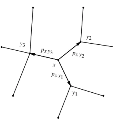
Remark 2.4 (Random walk). If (V, E, c) is given as in Definition 2.2, then for
(x, y)∈E, set
pxy:=
cxy
c(x) (2.6)
and note then {pxy} in (2.6) is a system of transition probabilities, i.e.,Pypxy = 1
for allx∈V (see Figure 2.1 below).
A Markov-random walk on V with transition probabilities (pxy) is said to be reversible iff there exists a positive functionec onV such that
e
c(x)pxy=ec(y)pyxfor all(x, y)∈E. (2.7)
x
y2
y1
y3
px y2
px y3
px y1
Fig. 2.1. Transition probabilitiespxy at a vertexx(inV)
Proof. Ifcis a conductance function onE (see Definition 2.1), then(pxy), defined in
(2.6), is a reversible walk. This follows fromcxy=cyx.
Conversely, if (2.7) holds for a system of transition probabilities (pxy =
=Prob(x7→y)), thencxy:=ec(x)pxyis a conductance function, where
e
c(x) =X
y∼x
cxy.
For results on reversible Markov chains, see e.g., [27].
3. ELECTRICAL CURRENT AS FRAME COEFFICIENTS
The role of the graph-network setting (V, E, c,HE)introduced above is, in part, to model a family of electrical networks; one application among others. Here G is a graph with vertices V, and edges E. Since we study large networks, it is helpful to take V infinite, but countable. Think of a network of resistors placed on the edges inG. In this setting, the functionsv(x,y)inHE, indexed by pairs of vertices, represent
dipoles. They measure voltage drop in the network through all possible paths between the two verticesxandy. Now the conduction functioncis given, and so (electrical) current equals the product of conductance and voltage drop; in this case voltage drop is computed over the paths made up of edges from xto y. For infinite systems
(V, E, c)the corresponding dipolesvxy arenot inl2(V), but they are always inHE;
see Lemma 3.4 below.
This result will be proved below. For general background references on frames in Hilbert space, we refer to [8, 12, 16, 24, 25, 30], and for electrical networks, see [3,4,9,15,29,33,35]. The facts on electrical networks we need are the laws of Kirchhoff and Ohm, and our computation of the frame coefficients as electrical currents is based on this, in part.
Definition 3.1. LetH be a Hilbert space with inner product denotedh·,·i, orh·,·i H when there is more than one possibility to consider. LetJ be a countable index set, and let{wj}j∈J be an indexed family of non-zero vectors inH. We say that{wj}j∈J
is a frame forH iff there are two finite positive constantsb1andb2such that
b1kuk2H ≤
X
j∈J
hwj, uiH
2≤b2kuk2H (3.1)
holds for allu∈H. We say that it is aParseval frame ifb1=b2= 1.
Lemma 3.2. If {wj}j∈J is a Parseval frame in H, then the (analysis) operator
A=AH :H −→l2(J),
Au= hwj, uiH
j∈J (3.2)
is well-defined and isometric. Its adjointA∗:l2(J)−→H is given by
A∗(γj)j∈J
:=X
j∈J
γjwj (3.3)
and the following hold:
1. The sum on the RHS in (3.3)is norm-convergent;
2. A∗:l2(J)−→H is co-isometric; and for allu∈H, we have
u=A∗Au=X
j∈J
hwj, uiwj, (3.4)
where the RHS in (3.4)is norm-convergent.
Proof. The details are standard in the theory of frames; see the cited papers above. Note that (3.1) for b1 = b2 = 1 simply states that A in (3.2) is isometric, and so
A∗A=I
H =the identity operator inH, and AA∗ =the projection onto the range ofA.
When a conductance function c:E →R+∪ {0} is given, we consider the energy Hilbert space HE (depending onc) with inner product and norm:
hu, viHE:=
1 2
X X
(x,y)∈E
cxy
u(x)−u(y)(v(x)−v(y)) (3.5)
and
kuk2HE=hu, uiHE =
1 2
X X
(x,y)∈E
cxy|u(x)−u(y)|
2
We shall assume that (V, E, c) isconnected (see Definition 2.1). It is shown that then (3.4)–(3.5) define HE as a Hilbert space of functions onV; functions defined modulo constants; see also 4 below.
Further, for any pair of verticesx, y∈V, there is a unique dipole vectorvxy∈HE
such that
hvxy, uiHE =u(x)−u(y) (3.7) holds for allu∈HE, see Lemma 3.4 below.
Remark 3.3. We illustrate this Parseval frame in Section 7.4 with a finite--dimensional example.
3.1. DIPOLES
Let(V, E, c,HE)be as described above, and assume that(V, E, c)is connected. Note that “vectors” in HE are equivalence classes of functions on V (= the vertex set in the graphG= (V, E)).
Lemma 3.4 ([19]). For every pair of vertices x, y ∈ V, there is a unique vector
vxy∈HE satisfying
hu, vxyiHE =u(x)−u(y) (3.8)
for allu∈HE.
Proof. Fix a pair of verticesx, yas above, and pick a finite path of edges(xi, xi+1)∈E such thatcxi,xi+1 >0, andx0=y,xn=x. Then
u(x)−u(y) =
nX−1
i=0
u(xi+1)−u(xi)
=
nX−1
i=0
1
√c xixi+1
√c
xixi+1(u(xi+1)−u(xi)) (3.9)
and, by the Schwarz inequality, we have the following estimate:
|u(x)−u(y)|2≤ nX−1
i=0
1 cxixi+1
!nX−1
j=0
cxjxj+1|u(xj+1)−u(xj)| 2
≤(Constxy)kuk2HE,
valid for all u∈HE, where we used (3.6) in the last step of this a priori estimate. But this states that the linear functional:
Lxy:HE∋u7−→u(x)−u(y) (3.10)
is continuous on HE w.r.t. the norm k·kH
E. Hence existence and uniqueness for
vxy∈HE follows from Riesz’ theorem. We get a uniquevxy∈HE such that
Remark 3.5. Letx, y∈V be as above, and letvxy ∈HE be the dipole. One checks,
using (2.1)–(2.2) that
∆vxy=δx−δy. (3.11)
But this equation (3.11) does not determinevxy uniquely. Indeed, ifw is a function
onV satisfying∆w= 0, i.e.,wis harmonic, thenvxy+walso satisfies eq. (3.11). (In
[20, 21] we studied when(V, E, c)has non-constant harmonic functions inHE.) The system of vectors vxy in (3.7) indexed by pairs of vertices carry a host of
information about the given system (V, E, c,HE), for example the computation of
resistance metric.
Lemma 3.6. Whenc (conductance)is given and assume(V, c)is connected, set
dc(x, y) := sup
(
1
kuk2HE
u∈HE, u(x) = 1, u(y) = 0
)
. (3.12)
Thendc(x, y)is a metric on V, and
dc(x, y) =kvxyk2HE, (3.13)
where the dipole vectors are specified as in (3.7).
Proof. Consider u∈ HE as in (3.12), i.e., u(x) = 1, u(y) = 0. Using (3.7) and the Schwarz inequality, we then get
1 =u(x)−u(y) =hvxy, uiHE
2
≤ kvxyk2HEkuk
2 HE.
Since we know the optimizing vectors in the Schwarz inequality, the desired formula (3.13) now follows from (3.12) and (3.7). But (3.12) is known to yield a metric and the lemma follows.
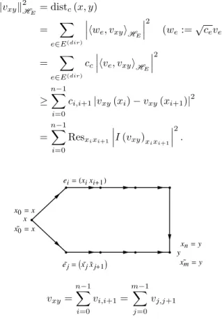
The next lemma offers a lower bound for the resistance metric between any two vertices when(V, E, c)is given. Given any two verticesxandy, we prove the following estimate: distc(x, y)≥sum of dissipation along any path of edges fromxto y.
Lemma 3.7. Let G= (V, E, c)be as before. For all finite paths
x0:=x→(ei)→xn:=y,
we have
distc(x, y)≥ nX−1
i=0
Resxixi+1
I(vxy)i,i+1
2
| {z }
dissipation
, (3.14)
where Res=1
Proof. In general there are many paths fromxto y whenxand y are fixed vertices (see Figure 3.1).
kvxyk2HE =distc(x, y)
= X
e∈E(dir)
hwe, vxyiHE
2
(we:=√ceve)
= X
e∈E(dir)
cc
hve, vxyiHE
2
≥ n−1
X
i=0
ci,i+1|vxy(xi)−vxy(xi+1)|2
=
n−1
X
i=0
Resxixi+1
I(vxy)x
ixi+1
2
.
x
y
x0=x
x0=x
xn=y
xm =y
ei=Hxixi+1L
ej=Ixjxj+1M
vxy= nX−1
i=0
vi,i+1=
mX−1
j=0
vj,j+1
Fig. 3.1. Two finite paths connectingxandy, whereei= (xixi+1),eej= (exjxej+1)∈E
Now pick an orientation for each edge, and denote by E(ori) the set of oriented edges.
Theorem 3.8. Let V, E, c, E(ori)andH
E be as above. Then the system of vectors
wxy:=√cxyvxy, indexed by(xy)∈E(ori), (3.15)
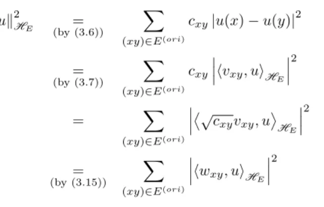
Proof. We will show that (3.1) holds for constants b1 = b2 = 1 for the vectors
w(xy)(xy)∈E(ori), see (3.7)–(3.15). Indeed, we have foru∈HE:
kuk2HE = (by(3.6))
X
(xy)∈E(ori)
cxy|u(x)−u(y)|2
=
(by(3.7))
X
(xy)∈E(ori)
cxy
hvxy, uiHE
2
= X
(xy)∈E(ori)
√cxyvxy, u
HE
2
=
(by(3.15))
X
(xy)∈E(ori)
hwxy, uiHE
2
which is the desired conclusion.
Remark 3.9. While the vectors wxy := √cxyvxy, (xy) ∈ E(ori), form a Parseval
frame in HE in the general case, typically this frame is not an orthogonal basis (ONB) in HE, although it is in Example 7.1 below.
To see when our Parseval frames are in fact ONBs, we use the following lemma.
Lemma 3.10. Let {wj}j∈J be a Parseval frame in a Hilbert space H, then kwjkHE≤1, and it is an ONB inH if and only ifkwjkH = 1for allj ∈J.
Proof. Follows from an easy application of
kuk2H =
X
j∈J
hwj, uiH
2
, u∈H. (3.16)
Plug inwj0 foruin (3.16).
Remark 3.11. Frames in HE consisting of our system (3.15) are not ONBs when resisters are configured in non-linear systems of vertices, for example, resisters in parallel. See Figure 3.2 and Example 7.4.
V =Band V =Z2
In these examples one checks that
1>kwxyk2HE =cxykvxyk 2
HE =cxy(vxy(x)−vxy(y)). (3.17)
That is the current flowing through each edgee= (x, y)∈E is <1, or equivalently the voltage-drop acrosseis<resistance
vxy(x)−vxy(y)<
1 ccy
=resistance.
Definition 3.12. LetV, E, c,HE be as above and foru∈HE, set
I(u)(xy):=cxy(u(x)−u(y)) for(x, y)∈E. (3.18)
By Ohm’s law, the functionI(u)(xy)in (3.18) represents the current in a network. A choice oforientation may be assigned as follows (three different ways): 1. The orientation of every (xy)∈E may be chosen arbitrarily.
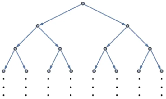
2. The orientation may be suggested by geometry; for example in a binary tree, as shown in Figure 3.3 below.
3. Or the orientation may be assigned by the experiment of inserting one Amp at a vertex, sayo∈V, and extracting one Amp at a distinct vertex, sayxdist∈V. We
then say that an edge (xy)∈E is positively oriented ifI(u)xy >0whereI(u)xy
is the induced current; see (3.18). See Figure 3.4 below.
Fig. 3.3. Geometric orientation (see also Figure 7.4 below)
o xdist
Corollary 3.13(Figure 3.4). Let(V, E, c,HE)be as above, and letE(ori)be assigned
as in(3)of Definition 3.12. Then everyu∈HEhas a norm-convergent representation
u= X
(xy)∈E(ori)
I(u)xyvxy. (3.19)
Proof. By Theorem 3.8 and Lemma 3.2, we have the following norm-convergent rep-resentation
u= X
(xy)∈E(ori)
hwxy, uiHEwxy, (3.20)
see (3.4). Now, by statements (3.15) and (3.18), we get
hwxy, uiHEwxy=I(u)xyvxy. (3.21)
Considering (3.20) and (3.21), the desired conclusion (3.19) then follows.
4. LEMMAS
Starting with a given network (V, E, c), we introduce functions on the vertices V, voltage, dipoles, and point-masses; and on the edgesE, conductance, and current. We introduce a system of operators which will be needed throughout, the graph-Laplacian
∆, and the transition operatorP. We show that there are two Hilbert spaces serving different purposes, l2(V), and the energy Hilbert spaceH
E; the latter depending on
choice of conductance function c.
Lemma 4.2 below summarizes the key properties of∆as an operator, both inl2(V) and inHE. The metric properties of networks(V, E, c)depend on HE (Lemma 4.3), and not onl2(V).
Recall that the graph-Laplacian ∆ is automatically essentially selfadjoint as a densely defined operator in l2(V), but not as a H
E operator [17, 21]. In Section 7
we compute examples where (∆,HE) has deficiency indices (m, m), m > 0. These results make use of an associated reversible random walk, as well as the transition operatorP.
Let (V, E, c)be as above; note we are assuming thatG= (V, E)is connected; so there is a pointo in V such that every x∈ V is connected to o via a finite path of edges. We will setV′ :=V\ {o}, and considerl2(V)andl2(V′). Ifx∈V, we set
δx(y) =
(
1 ify=x,
0 ify6=x. (4.1)
SetHE:=the set of all functionsu:V →Csuch that
kuk2HE:=
1 2
X X
(x,y)∈E
cxy|u(x)−u(y)|
2
and we note ([19]) thatHE is a Hilbert space. Moreover, for allx, y∈V, there is a real-valued solutionvxy∈HE to the equation
∆vx,y =δx−δy. (4.3)
Ify=o, we set vx:=vx,o, and note
∆vx=δx−δo. (4.4)
In this case, we assume thatvxis defined only for x∈V′.
Definition 4.1. Let V, E, c, o,∆,{vx}x∈V′
be as above, and set
D2:=spanδxx∈V (4.5)
and
DE :=spanvxx∈V′ , (4.6)
where by “span” we mean of all finite linear combinations.
Lemma 4.2. The following hold:
1. h∆u, vil2 =hu,∆vil2 for allu, v∈D2;
2. h∆u, viHE =hu,∆viHE for allu, v∈DE; 3. hu,∆uil2 ≥0for all u∈D2;
4. hu,∆uiHE≥0 for allu∈DE, where foru, v∈HE we set
hu, viHE =
1 2
X X
(x,y)∈E
cxy(u(x)−u(y)) (v(x)−v(y)). (4.7)
Moreover, we have
5. hvx,y, uiHE=u(x)−u(y)for all x, y∈V.
Finally, 6.
δx(·) =c(x)vx(·)−
X
y∼x
cxyvy(·) for all x∈V′.
Proof. (2) We haveh∆u, viHE=hu,∆viHE, for allu, v∈DE. Set vx:=vxo, whereo
is a fixed base-point inV,V′:=V\ {o}, so∆v
x=δx−δo,x∈V′. Setu=Px∈V′ξxvx,
v=Px∈V′ηxvx, where the summations are finite by convention. Then h∆u, viHE=
X
V′
X
V′
ξxηyhδx−δo, vyiHE
=X
V′
X
V′
ξxηy (δx(y)−δx(o)
| {z }
=0
)−(δo(y)
| {z }
=0
−δo(o)
| {z }
=1
)
=X
V′
X
V′
ξxηy(δxy+ 1)
=X
V′
ξxηy+
X
V′
ξx
X
V′
ηy
Lemma 4.3. Let (V, E, c, o)be as above. Then the function
Nc(x, y) :=kvx−vyk2HE (4.8)
is conditionally negative definite, i.e., for all finite system {ξx} ⊆ C such that
P
x∈V′ξx= 0, we have
X
x
X
y
ξxξyNc(x, y)≤0. (4.9)
Proof. Compute the LHS in (4.9) as follows. IfPξx= 0, we have
X
ξxξyNc(x, y)
=−X Xξxξyhvx, vyiHE−
X X
ξxξyhvy, vxiHE
=−2X
x
ξxvx
2
HE.
We show also the following
Lemma 4.4 ([19]).
u∈HE hu, δxi
HE= 0for allx∈V =
u∈HE∆u= 0 . (4.10)
WhenN is a fixed negative definite function, we get an associated Hilbert space HN by completing finitely supported functions ξ on V subject to the condition
P
x∈V ξx= 0, under the inner product
kξk2HN :=−
X
x
X
y
ξxξyN(x, y)
and quotienting out with X
x
X
y
ξxξyN(x, y) = 0.
Lemma 4.5. Assume (V, E, c) is connected. If a negative definite function N on
V ×V satisfiesN =Nc, then
HN
c=HE, (4.11)
whereHE is the energy Hilbert space from 3 defined on the prescribed functions.
Proof. By Lemma 4.3, we have
kξk2HNc =
X
x∈V′
ξxvx
2
HE, (4.12)
wherevx=voxis a system of dipoles corresponding to a fixed base pointo∈V, and
V′=V\ {o}, and
Hence, we need only prove that all the finite summations Px∈V′ξxvx subjecting to
P
x∈V′ξx= 0are dense inHE. But if u∈HE,u∈Px∈V′ξxvx
Px∈V′ξx= 0
⊥
(the orthogonal-complement), then
hvx, uiHE− hvy, uiHE= 0
for all x, y ∈ V′. Hence by (4.13) we get u(x) = u(y) for all pairs x, y ∈ V′; and u(x) =u(o), x∈V′. Since (V, E, c)is connected, it follows that uis constant. But
with the normalization vx(o) = 0 (x∈V′), we conclude thatumust be zero.
Lemma 4.6. Let (V, E, c)be a connected network, and let HE be the energy Hilbert
space. Then, for allf ∈HE and x∈V, we have
hδx, fiHE = (∆f) (x). (4.14)
Proof. We compute LHS(4.14) with the use of eq. (4.7) in Lemma 4.2. Indeed,
hδx, fiHE = (4.7)
1 2
X X
(st)∈E
cst(δx(s)−δx(t)) (f(s)−f(t))
= X
t∼x
cxt(f(x)−f(t)) = (∆f) (x),
where we used (2.2) in Definition 2.2 in the last step.
Corollary 4.7. Let (V, E, c)be as above. Then
hδx, δyiHE = e
c(x) =Pt∼xcxt ify =x,
−cxy if(xy)∈E,
0 if(xy)∈E andx6=y.
(4.15)
Proof. Immediate from the lemma.
Corollary 4.8. Let (V, E, c,∆) be as above. Then
HE⊖ {δx|x∈V}={u∈HE|∆u= 0}. (4.16)
Proof. This is immediate from (4.14) in Lemma 4.6. (Note that “⊖” in (4.16) means ortho-complement.)
Corollary 4.9. Let (V, E, c,∆) be as above. Then, for everyx∈V, we have
X
y∼x
cxyvxy=δx. (4.17)
5. THE HILBERT SPACESHE ANDl2(V′), AND OPERATORS BETWEEN THEM
The purpose of this section is to prepare for the two results (Sections 5 and 6) on factorization to follow.
Definition 5.1. Let V, E, c, o,{vx}x∈V′
be specified as in Sections 2–4, wherec is a fixed conductance function. Set
D′
l2 :=all finitely supported functionsξonV′such that
X
x
ξx= 0. (5.1)
Then assuming that V is infinite, we conclude thatD′
l2 is dense in l2(V′).
Lemma 5.2. For(ξx)∈Dl′2, set
K(ξ) := X
x∈V′
ξxvx∈HE. (5.2)
ThenK(=Kc)is a densely defined, and closable operator
K:l2(V′)−→HE
with domainD′
l2.
Proof. We must prove that the norm-closure of the graph of K in l2×H
E is again
the graph of a linear operator; equivalently, iflimn→∞
ξ(n)
l2 = 0, ξ (n)∈D
l2; and if there existsu∈HE such that
lim
n→∞
Kξ(n)
−u
HE= 0, (5.3)
thenu= 0inHE.
We prove this by establishing a formula for an adjoint operator,
K∗:H
E−→l2(V′)
having as its domain
( X
x
ξxvx
finite sums,ξx∈Csuch thatPxξx= 0
)
. (5.4)
Setting
K∗ X
x
ξxvx
!
= (ζx),
where
ζx=
X
y
on the space in (5.4), we show that this is a well-defined, densely defined, linear operator, and that
D
K∗ X
x
ξxvx
, ηE
l2 =
D X
x
ξxvx, Kη
E
HE (5.6)
holds for all η ∈D′
l2. This shows that a well-defined adjointK∗ operator exists (by (5.5)), and that therefore the implication in (5.3) is valid.
Now letξ, η∈D′
l2 as in (5.1). Then
(LHS)(5.6) =
* X
y
hvx, vyiHEξy, η +
l2
= X
x
X
y
ξyhvy, vxiHEηx
=
* X
y
ξyvy,
X
x
ηxvx
+
HE
=
(by(5.2))
* X
y
ξyvy, Kη
+
HE
= (RHS)(5.6).
6. THE FRIEDRICHS EXTENSION
Below we fix a conductance function c which turns the system(V, E, c) into a con-nected network (see Section 2), and we will study the c-graph Laplacian ∆ in HE, the energy Hilbert space.
Notice that ∆ will then be densely defined in HE, see Definition 4.1 and Lemma 4.2. Below we study the Friedrichs extension of ∆ when it is defined on its natural dense domainDE inHE.
Let(V, E, c, o,{vx},∆)be as above, i.e.,
• G
(
V =set of vertices, assumed countable infiniteℵ0,
E=edges,VassumedE−connected,
• c:E−→R+∪ {0}a fixed conductance function,
• ∆ (:= ∆c)the graph Laplacian,
• o∈V a fixed base-point such that∆vx=δx−δo,
• V′:=V\{o},
Recall we proved in Section 2 that∆is a semibounded Hermitian operator with dense domainDE inHE.
In this section, we shall be concerned with its Friedrichs extension, now denoted
∆F ri; for details on the Friedrichs extension, see e.g., [1, 10]; and, in the special case
of(∆,HE), see [19, 21].
In all cases, we have that ∆,∆F ri, and ∆∗ as operators in HE act on subspaces
of functions onV via the following formula:
(∆u) (x) =X
y∼x
cxy(u(x)−u(y)), (6.1)
whereuis a function on the vertex setV.
Lemma 6.1. As an operator inHE, the graph Laplacian∆ (with domainDE)may,
or may not, be essentially selfadjoint. Its deficiency indices are (m, m), where
m= dimu∈HE∆u=−u . (6.2)
Proof. Recall that ifS is a densely defined operator in a Hilbert spaceH such that
hu, Sui ≥0 for allu∈dom(S), (6.3)
then S will automatically have indices (m, m) where m = dim (N (S∗+I)), and whereS∗ denotes the adjoint operator, i.e.,
dom(S∗) =nu∈H there existsC <∞
such that |hu, Sϕi| ≤Ckϕkfor allϕ∈dom(S)o.
(6.4)
We may apply this toH =HE, andS:= ∆on the domainDE. One checks that, ifu∈dom(S∗), i.e.,u∈dom((∆|
DE)∗), then
(S∗u) (x) = X
y∈E(x)
cxy(u(x)−u(y)),
(i.e., the pointwise action of∆on functions) and the conclusion in (6.2) follows from the assertion aboutN (S∗+I).
Corollary 6.2. Let pxy:= cxy
c(x) be the transition-probabilities in Remark 2.4(see also
Figure 2.1), and let
(P u) (x) :=X
y∼x
pxyu(y) (6.5)
be the corresponding transition operator, accounting for thep-random walk on (V, E). Let(∆,HE)be theHE-symmetric operator with domainDE, see Definition 4.1. Then
(∆,HE) has deficiency indices (m, m), m >0, if and only if there is a function u
onV,u6= 0,u∈HE satisfying
1 + 1
c(x)
Proof. Since(∆|DE)∗acts pointwise on functions onV (see Lemma 6.1), we only need to verify that the equation−u= ∆utranslates into (6.6), but we have:
−u(x) =c(x)u(x)−X y∼x
cxyu(y)⇐⇒
1 + 1
c(x)
u(x) =X
y∼x
cxy
c(x)u(y)
which is the desired eq. (6.6).
Forufrom (6.6) to be indom((∆|DE)∗)we must have
X
(xy)∈E
cxy|u(x)−u(y)|
2
<∞
as asserted.
In the discussion below, we use that both operators ∆ and P take real valued functions on V to real valued functions, and that P is positive, satisfying P1 =1, where1is the constant function “one” onV.
Lemma 6.3. If uis a non-zero real valued function on V satisfying (6.2), or equiv-alently (6.6), and ifp∈V satisfiesu(p)6= 0, then there is an infinite path of edges
(xixi+1)∈E such that x0=p, and
u(xk+1)≥
k
Y
i=0
1 + 1
c(xi)
u(p). (6.7)
Proof. We may assume without loss of generality that u(p) > 0. Set x0 = p, and
x1:= arg max{u(y)|y∼x0}, sou(x1) = maxu
E(x0). Then
u(x1)≥
X
y∼x0
px0yu(y) = (P u) (x0) =
1 + 1
c(x0)
u(x0),
where we used (6.6) in the last step.
Now for the induction: Supposex1, . . . , xk have been found as specified; then set
xk+1:= arg max{u(y)|y∼xk}, so
u(xk+1)≥(P u) (xk) =
1 + 1
c(xk)
u(xk).
A final iteration then yields the desired conclusion (6.7).
Remark 6.4. In Section 7.1 below, we illustrate a family of systems(V, E, c), where
∆inHEhas indices(1,1). In these examples,V =Z+∪{0}, and the edgesEconsists of nearest neighbor links, i.e., if x∈Z+,
Lemma 6.5. A functionuonV is in the domain of ∆F ri (the Friedrichs extension) if and only if uis in the completion ofDE with respect to the quadratic form
DE ∋ϕ7−→ hϕ,∆ϕi
HE∈R+∪ {0} (6.8)
and
∆u∈HE. (6.9)
Proof. The assertion follows from an application of the characterization of ∆F ri in
[1, 10] combined with the following fact: If ϕ = Px∈V ξxvx is a finite sum with
coefficient(ξx)satisfyingPxξx= 0, then
hϕ,∆ϕiHE =
X
x∈V′ |ξx|
2
. (6.10)
Moreover, eq. (6.9) holds if and only if
k∆uk2HE :=
1 2
X
(x,y)∈E
cxy|(∆u) (x)−(∆u) (y)|2<∞.
We now prove formula (6.10). Assumeϕ=Px∈V′ξxvxis as stated. Then
hϕ,∆ϕiHE =
DX
xξxvx,∆
X
xξyvy
E
HE
=DX
xξxvx,
X
yξy(δy−δo)
E
HE
=X
x
X
yξxξyhvx, δyiHE (since
X
yξy = 0)
=X
x|ξx|
2
.
Lemma 6.6. LetHE denote the completion ofDE, and letD′
l2 be the dense subspace
inl2(V′), given by P
x∈V′ξx= 0,Px|ξx|2<∞. Set
L(ξx) :=
X
x
ξxδx. (6.11)
Then L : l2(V′) −→ H
E is a closable operator with dense domain Dl′2 and the
corresponding adjoint operator
L∗:HE −→l2(V′)
satisfies
L∗X
x∈V′ξxvx
Proof. To prove the assertion, we must show that, ifξis a finitely supported function onV′ such thatP
x∈V′ξx= 0, then
hL(ξ), uiHE=hξ, ηil2, (6.13)
where
u= X
y∈V′
ηyvy. (6.14)
We prove (6.13) as follows:
(LHS)(6.13) = D∆(X
xξxvx),
X
yηyvy
E
HE
= DX
xξxvx,∆(
X
yηyvy)
E
HE
= X
xξxηx= (RHS)(6.13),
where we used formula (6.10) in the last step of the computation.
Remark 6.7. To understand ∆ as an operator in the respective subspaces of HE recall thatHE contains two systems of vectors{δx}and{vx} both indexed byV′.
Neither of the two systems is orthogonal in the inner product of HE.
We havehvx, vyiHE =vx(y) =vy(x). Recall our normalizationvx(o) = 0, where
ois the fixed base-point. Moreover (see Corollary 4.7),
hδx, δyiHE =
−cxy if(x, y)∈E,
c(x) ifx=y, 0 otherwise,
and
hδx, vyiHE =
(
δxy ifx, y∈V′, −1 ifx=o, y∈V′.
Corollary 6.8. If x∈V′, thenδ
x∈HE and
δx(·) =c(x)vx(·)−
X
y∼x
cxyvy(·). (6.15)
Proof. To show this, it is enough to check equality of
LHS(6.15), vxH
E=
RHS(6.15), vxH
E for allx∈V ,
and this follows from an application of the formulas in Remark 6.7 above.
(i) LL∗ is selfadjoint, and
(ii) LL∗= ∆
F ri.
Proof. Conclusion (i) follows for every closed operatorLwith dense domain, we have thatLL∗ is selfadjoint. To prove (ii), we must verify that
LL∗u= ∆u for all u∈DE′ . (6.16)
Letu=Px∈V′ξxvx be a finite sum such thatPxξx= 0. Then
LL∗u =
(by(6.12))Lξ
=
(by(6.11))
X
x∈V′
ξxδx
=
(since Pξx=0) X
x∈V′
ξx(δx−δo)
=
(by(6.11))
X
x∈V′
ξx∆vx
=
since finite sum∆
X
x
ξxvx
!
= ∆u= (RHS)(6.16).
Corollary 6.10. We have the Greens-Gauss identity:
(∆y(hvx, vyi)) (z) =δxz for allx, y, z∈V′. (6.17)
The inner products hvx, vyi := hvx, vyiHE constitute the Gramian of the frame
Theorem 3.8.
Proof.
(LHS)(6.17)=
X
w∼z
czw hvx, vziHE− hvx, vwiHE
= X
w∼z
czw(vx(z)−vx(w))
= (∆vx) (z)
= (δx−δo) (z) =δxz = (RHS)(6.17),
6.1. THE OPERATORP VERSUS∆
Let (V, E, c) be a network with vertices V, edges E, and conductance function
c:E→R+∪ {0}. Setting
e
c(x) :=X
y∼x
cxy, pxy:=
cxy
ec(x), and
(∆u) (x) =X
y∼x
cxy(u(x)−u(y)),
(P u) (x) =X
y∼x
pxyu(y),
(6.18)
we have the connection
∆ =ec(I−P), and (6.19)
P =I−1
e
c∆ (6.20)
from (6.6) in Corollary 6.2.
Theorem 6.11. LetHE (depending onc)be the energy Hilbert space, and setl2(ec) =
l2(V,
e
c) =all functions on V with inner product
hu1, u2il2(ec)=
X
x∈V
e
c(x)u1(x)u2(x). (6.21)
Then
1. ∆ is Hermitian in HE, but not in l2(ec),
2. P is Hermitian inl2(
e
c)and in HE.
Proof. The first half of conclusion (1) is contained in Lemma 4.2. To show thatP is also Hermitian inHE, use (6.20) and the following lemma applied tof =1
e
c.
Lemma 6.12. Let ∆,P, andHE be as above, and let f be a function on V, then
h(f∆)vx, vyiHE=hvx,(f∆)vyiHE. (6.22)
Proof. We compute as follows, using (3.11): LHS(6.22)=hf(·) (δx−δo), vyiHE
= (f(·) (δx−δo)) (y)−(f(·) (δx−δo)) (o)
=f(y)δxy+f(o)
for all verticesx, y∈V′=V\ {o}, whereois a fixed choice of base-point in the vertex
Proof of Theorem 6.11, part (2). We show that
h(P u1), u2il2(ec)=hu1,(P u2)il2(ec)
for all finitely supported functions u1, u2 onV.
But this follows from the assumptionec(x)pxy=ec(y)pyx (reversible). Since
X
x
e
c(x)pxy=
X
x
e
c(y)pyx=ec(y)
X
x
pyx=ec(y),
i.e., the functionec is left-invariant forP, viz:ecP =ec viewingP = (pxy)as a Markov
matrix.
The final assertion, that∆is not Hermitian inl2(
e
c)follows from Lemma 4.2, and the fact that∆does not commute with the multiplication operator f =1
ec. Corollary 6.13. Let(P u) (x) =Py∼xpxyu(y)be the transition operator, where
pxy=
cxy
e
c(x) (6.23)
is defined for(xy)∈E,c is a fixed conductance on (V, E), and
e
c(x) =X
y∼x
cxy. (6.24)
ThenP is selfadjoint and contractive inl2(V,ec).
Proof. We proved in Lemma 4.2 (3) that hu,∆uil2 ≥ 0 holds for all u ∈ l2 where
h·,·il2 referes to the un-weighted l2-inner product. The connection between the two inner products is as follows:hu,ecuil2=kuk
2
l2(ec) which yields the following: Using (6.23) and (6.24), we get
P u=u−1
e
c∆u, (6.25)
soecP u=ecu−∆u, and as a point-wise identity on V. Hence
hu, P uil2(ec)=hu,ecu−∆uil2
=kuk2l2(ec)− hu,∆uil2
≤ kuk2l2(ec) (by Lemma 4.2 (3))
holds for allu∈l2(
e
c).
Since we also proved that P (see eq. (6.25)) isl2(
e
c)-Hermitian, we conclude that it is contractive and selfadjoint in the Hilbert spacel2(
e
c), as claimed.
Lemma 6.14. Let(V, E, c, p),∆, andP be as above. Then a functionuonV satisfies
Proof. Immediate from∆u= ˜c(u−P u)(eq. (6.19)).
Corollary 6.15. Let(V, E, c)be as above, and set
pxy:=
cxy
e
c(x), (xy)∈E, (6.26)
whereec(x) :=Py∼xcxy. Fix o∈V and consider the dipoles (vx)x∈V′,V′ =V\ {o},
where
hvx, uiHE =u(x)−u(o) for allx∈V′. (6.27)
Setting
(P u) (x) =X
y∼x
pxyu(y), (6.28)
we get
P vx=
X
y∼x
pxyvy, (6.29)
and the following implication holds for the dense subspace DE inHE:
u∈DE =⇒P u∈DE, (6.30)
where
DE:=
( X
x
ξxvx
ξx∈C, finitely supported on V′, such that
X
x
ξx= 0
)
. (6.31)
Proof. A direct computation shows that (6.29) must hold as an identity on functions onV, up to an additive constant.
Our assertion is that working in the Hilbert space HE implies that the additive constant is zero. This amounts to verification of the implication (6.30), i.e., that
X
x
ξx= 0 =⇒
X
y
X
x
ξxpxy
!
= 0 (6.32)
for all finitely supported functions. But we have
X
y
X
x
ξxpxy
!
=X
x
ξx
X
y
pxy
!
=X
x
ξx= 0
which is the desired assertion (6.32). Hence (6.30) follows.
7. EXAMPLES
The purpose of the first example is multi-fold.
function on the edges(n, n+ 1), and we get non-trivial models where explicit formulas are possible and transparent. For example, we can write down the dipoles vxy as
functions onV, and the corresponding resistance metric; see the formulas relating to Figure 7.1. Among all the conductance functions we characterize the cases of reversible Markov models where the left/right transition probabilities are the same for all vertex points. In Section 7.2 (the binomial model) we accomplish the same characterization of the cases of reversible Markov models where the left/right transition probabilities are the same for all vertex points, but now every vertex in the binary tree has three nearest neighbors.
In Section 7.4 we give a finite graph(V, E, c)as a triangular configuration, conduc-tancecdefined on the edges of the triangle, and we find the Parseval frame (thereby illustrating Theorem 3.8).
The examples below illustrate the following: When a graph network (V, E, c) is infinite, then the dipolesvxy as functions onV will not lie in the Hilbert spacel2(V).
Hence another justification for the energy Hilbert spaceHE.
7.1. V ={0} ∪Z+
ConsiderG= (V, E, c), whereV ={0} ∪Z+. Every sequencea1, a2, . . .inR+ defines a conductancecn−1,n:=an,n∈Z+, i.e.,
0oo a
1 //1oo a2 //2oo a3 //3 · · · noo an+1//n+ 1 · · ·
The dipole vectorsvxy (forx, y∈N) are given by
vxy(z) =
0 ifz≤x,
−Pzk=x+1a1k ifx < z < y,
−Pyk=x+1a1k ifz≥y.
See Figure 7.1.
x z y
It follows from Lemma 3.6 that the resistance metricdist(=dc=da)is as follows:
dist(x, y) =
0 ifx=y,
1 ax+1
+· · ·+ 1 ay
| P {z }
x<k≤y
1
ak
ifx < y.
Note that V = Z+ ∪ {0} with the resistance metric described above yields a
bounded metric space if and only if
∞
X
n=1
1 an
<∞. (7.1)
The corresponding graph Laplacian has the following matrix representation:
a1 −a1
−a1 a1+a2 −a2
−a2 a2+a3 −a3 0
−a3 a3+a4 . ..
. .. . .. −an
−an an+an+1 −an+1
0 −an+1 . .. . ..
. .. . .. . .. . .. , (7.2) that is,
(∆u)0 =a1(u0−u1),
(∆u)n =an(un−un−1) +an+1(un−un+1),
= (an+an+1)un−anun−1−an+1un+1 for all n∈Z+.
(7.3)
Lemma 7.1. Let G = (V, c, E) be as above, where an := cn−1,n, n ∈ Z+. Then
u∈HE is the solution to ∆u=−u(i.e., uis a defect vector of ∆)if and only if u
satisfies the following equation:
∞
X
n=1
anhvn−1,n, uiHE(δn−1(s)−δn(s) +vn−1,n(s)) = 0 for all s∈Z+, (7.4)
where
kuk2HE =
∞ X n=1 an
hvn−1,n, uiHE
2
Proof. By Theorem 3.8, the set√anvn−1,n
∞
n=1 forms a Parseval frame inHE. In fact, the dipole vectors are
vn−1,n(s) =
(
0 s≤n−1
− 1
an s≥n
, n= 1,2, . . . , (7.6)
and so√anvn−1,n
∞
n=1 forms an ONB inHE, andu∈HE has the representation
u= ∞
X
n=1
anhvn−1,n, uiHEvn−1,n
(see (3.4)). Therefore,∆u=−uif and only if
∞
X
n=1
anhvn−1,n, uiHE(δn−1(s)−δn(s)) =−
∞
X
n=1
anhvn−1,n, uiHEvn−1,n(s)
for alls∈Z+, which is the assertion.
Conjecture 7.2. Consider∆as above as an operator inHE(depending oncn,n−1=
an). Then∆ is essentially selfadjoint(inHE)if and only if P
∞
n=1a1n =∞. If (7.1)
holds, the indices are (1,1).
Remark 7.3. Below we compute the deficiency space in an example with index values
(1,1).
Lemma 7.4. Let (V, E, c={an})be as above. LetQ >1 and setan :=Qn,n∈Z+.
Then∆ has deficiency indices(1,1). Proof. Suppose∆u=−u,u∈HE. Then,
−u1=Q(u1−u0) +Q2(u1−u2)⇐⇒u2=
1 Q2+
1 +Q Q
u1−
1 Qu0,
−u2=Q2(u2−u1) +Q3(u2−u3)⇐⇒u3=
1 Q3 +
1 +Q Q
u2−
1 Qu1,
and by induction,
un+1=
1 Qn+1 +
1 +Q Q
un−
1
Qun−1, n∈Z+,
i.e.,uis determined by the following matrix equation:
un+1
un
=
1
Qn+1 + 1+Q Q − 1 Q 1 0 un
un−1
The eigenvalues of the coefficient matrix are
λ±= 1 2
1
Qn+1 +
1 +Q
Q ±
s
1 Qn+1 +
1 +Q Q 2 − 4 Q ∼ 1 2
1 +Q
Q ± Q −1 Q = 1 1 Q
asn→ ∞.
Equivalently, asn→ ∞, we have
un+1∼
1 +Q Q
un−
1
Qun−1=
1 + 1 Q
un−
1 Qun−1,
and so
un+1−un∼
1
Q(un−un−1).
Therefore, for the tail-summation, we have
X
n
Qn(un+1−un)2=const
X
n
(Q−1)2 Qn+2 <∞
which implies kukHE<∞.
Next, we give a random walk interpretation of Lemma 7.4. See Remark 2.4 and Figure 2.1.
Remark 7.5 (Harmonic functions in HE). Note that in Example 7.1 (Lemma 7.4), the space of harmonic functions in HE is one-dimensional. In fact if Q >1 is fixed,
then
u∈HE∆u= 0
is spanned byu= (un)∞n=0,un= Q1n,n∈N; and of coursek1/Q
n k2
HE<∞.
Proof. This is immediate from Lemma 6.14.
Remark 7.6. For the domain of the Friedrichs extension∆F ri, we have
dom(∆F ri) =
f ∈HE| (f(x)−f(x+ 1))Qx∈l2(Z+) , (7.7)
i.e.,
dom(∆F ri) =
(
f ∈HE
∞ X x=0
|f(x)−f(x+ 1)|2Q2x< ∞
)
.
Proof. By Theorem 3.8, we have the following representation, valid for allf ∈HE:
f =X
x
f, Qx2v
(x,x+1)HEQ
x
2v (x,x+1)
=X
x
and
hf,∆fiHE=
X
x
|f(x)−f(x+ 1)|2Q2x.
The desired conclusion (7.7) now follows from Theorem 6.9 above and the character-ization of∆F ri (see e.g. [1, 10]).
Definition 7.7. LetG= (V, E, c)be a connected graph. The set of transition prob-abilities(pxy)is said to be reversible if there existsc:V →R+ such that
c(x)pxy=c(y)pyx, (7.8)
and then
cxy:=c(x)pxy (7.9)
is a system of conductance. Conversely, for a system of conductance(cxy)we set
c(x) :=X
y∼x
cxy (7.10)
and
pxy:=
cxy
c(x), (7.11)
and so(pxy)is a set of transition probabilities. See Figure 7.2 below.
x
y
y¢ cxy
cxy¢ x
y
y¢ px y
px y¢
cxy,y∼x transition probabilities
Fig. 7.2. Neighbors ofx
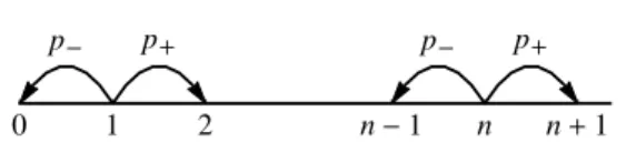
Recall the graph Laplacian in (7.3) can be written as
(∆u)n=c(n) (un−p−(n)un−1−p+(n)un+1) for all n∈Z+, (7.12)
where
c(n) :=an+an+1 (7.13)
and
p−(n) := an
c(n), p+(n) := an+1
c(n) (7.14)
p+
p- p- p+
0 1 2 n-1 n n+1
Fig. 7.3. The transition probabilitiesp+, p−, in the case of constant transition probabilities, i.e.,p+(n) =p+, andp−(n) =p−for alln∈Z+
In the case an =Qn, Q >1, as in Lemma 7.4, we have
c(n) :=Qn+Qn+1, (7.15)
and
p+:=p+(n) = Q
n+1
Qn+Qn+1 =
Q
1 +Q, (7.16)
p−:=p−(n) = Q
n
Qn+Qn+1 =
1
1 +Q. (7.17)
For alln∈Z+∪ {0}, set
(P u)n:=p−un−1+p+un+1. (7.18)
Note(P u)0=u1. By (7.12), we have
∆ =c(1−P). (7.19)
In particular,p+>12, i.e., a random walker has probability>12 of moving to the right. It follows that
travel time(n,∞)
| {z }
=dist to∞
<∞,
and so∆ is not essentially selfadjoint, i.e., indices(1,1).
Lemma 7.8. Let (V, E,∆(= ∆c))be as above, where the conductance c is given by
cn−1,n =Qn,n∈Z+,Q >1 (see Lemma 7.4). For allλ >0, there exists fλ∈HE satisfying ∆fλ=λfλ.
Proof. By (7.19), we have∆fλ=λfλ⇐⇒P fλ= 1−λc
fλ, i.e.,
1
1 +Qfλ(n−1) + Q
1 +Qfλ(n+ 1) =
1−Qn−1(1 +λ Q)
fλ(n)
and so
fλ(n+ 1) =
1 +Q
Q −
λ Qn
fλ(n)−
1
Qfλ(n−1). (7.20)
f(n+ 1) f(n) = 1+Q Q − λ Qn −Q1
1 0
f(n) f(n−1)
∼ 1+Q Q − 1 Q 1 0 f(n) f(n−1)
, asn→ ∞.
The eigenvalues of the coefficient matrix are given by
λ±∼ 1
2
1 +Q
Q ± Q −1 Q = 1 1 Q
asn→ ∞.
That is, asn→ ∞,
fλ(n+ 1)∼
1 +Q Q
fλ(n)−
1
Qfλ(n−1),
i.e.,
fλ(n+ 1)∼
1
Qfλ(n) ; (7.21)
and so the tail summation of kfλk
2
HE is finite. (See the proof of Lemma 7.4.) We conclude thatfλ∈HE.
Corollary 7.9. Let(V, E,∆)be as in the lemma. The Friedrichs extension∆F rihas continuous spectrum[0,∞).
Proof. Fixλ≥0. We prove that if∆fλ=λfλ, f ∈HE, thenfλ∈/ dom(∆F ri).
Note for λ= 0, f0 is harmonic, and sof0=k
1
Qn ∞
n=0 for some constant k6= 0. See Remark 7.5. It follows from (7.7) thatf0∈/dom(∆F ri).
The argument for λ >0 is similar. Since asn→ ∞,fλ(n)∼ Q1n (eq. (7.21)), so
by (7.7) again, fλ∈/ dom(∆F ri).
However, if λ0< λ1in [0,∞)then
λ1
Z
λ0
fλ(·)dλ∈dom(∆F ri) (7.22)
and so everyfλ,λ∈[0,∞), is a generalized eigenfunction, i.e., the spectrum of∆F ri
is purely continuous with Lebesgue measure, and multiplicity one. The verification of (7.22) follows from eq. (7.20), i.e.,
fλ(n+ 1) =
1 +Q
Q −
λ Qn
fλ(n)−
1
Qfλ(n−1). (7.23)
Set
F[λ0,λ1]:=
λ1
Z
λ0
Then by (7.23) and (7.24),
F[λ0,λ1](n+ 1) =
1 +Q
Q F[λ0,λ1](n)−
1 Qn
λ1
Z
λ0
λfλ(n)dλ−
1
QF[λ0,λ1](n−1)
andRλ1
λ0 λfλdλ is computed using integration by parts.
Remark 7.10 (Krein extension). Set
dom(∆Harm) :=dom(∆) +Harmonic functions,
∆Harm:= ∆∗dom(∆Harm).
Then∆Harm⊃∆is a well-defined selfadjoint extension of∆. It is semibounded, since
ϕ+h,∆Harm(ϕ+h)HE=hϕ+h,∆ϕiHE=hϕ,∆ϕiHE≥0
for allϕ∈dom(∆), andhharmonic. In fact∆Harmis the Krein extension.
7.2. A REVERSIBLE WALK ON THE BINARY TREE (THE BINOMIAL MODEL)
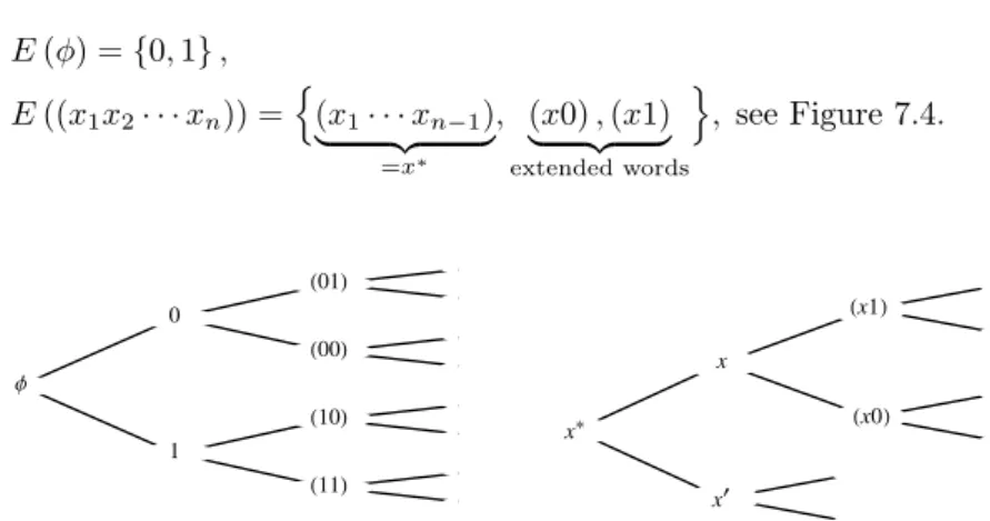
Consider the binary tree as a setV of vertices. To get a graph G= (V, E), take for edgesE the nearest neighbor lines as follows:
V :={o=φ,(x1x2· · ·xn), xi∈ {0,1},1≤i≤n}, (7.25)
and
E(φ) ={0,1},
E((x1x2· · ·xn)) =
n
(x1· · ·xn−1)
| {z }
=x∗
, (x0),(x1)
| {z }
extended words
o
, see Figure 7.4.
Φ
1 0
H11L H10L H00L H01L
x*
x¢ x
Hx0L Hx1L
Now fix transition probabilities at o = φ, and at the vertices V′ = V\ {φ} as
follows:
Prob(x→(x0)) =p0, Prob(x→(x1)) =p1, Prob(x→(x∗)) =p−
(7.26)
with0< p0<1(see Figure 7.4) such thatp0+p1+p−= 1, see Figure 7.5.
x
x*
Hx0L Hx1L
p
-p1
p2
Fig. 7.5. Transition probabilities at a vertexx∈V′. The reversible case with three nearest neighbors
Forx∈V′, set
F0(x) = #{i|xi= 0}, F1(x) = #{i|xi = 1}, (7.27)
and
|x|:=x1+x2+· · ·+xnso thatF0(x) +F1(x) =|x| for allx∈V′. (7.28) Further, define the functionc:V →R+ as follows:
c(x) =p
F0(x)
0 p
F1(x) 1
p|−x|
for all x∈V′. (7.29)
Lemma 7.11. With the transition probabilities defined in (7.26), it follows that the corresponding walk on V is reversible via the function c:V →R+ defined in (7.29),
i.e., we have the following identity for any edge(xy) inG= (V, E):
c(x)Prob(x→y) =c(y)Prob(y→x). (7.30)
Proof. This follows from a direct inspection of the cases (see also Figures 7.4 and 7.5).
For(xy)∈E, using (7.29)–(7.30), setcxy:=c(x)Prob(x→y), and
(∆u) (x) :=X
y∼x
cxy(u(x)−u(y)). (7.31)
Corollary 7.12. Ifmin (pi)> p−, then∆ in(7.31)has deficiency indices(1,1), i.e., the non-zero solution uto−u= ∆uis inHE; i.e.,0<kukH
E<∞.
Proof. The analysis here is analogous to the one above in Example 7.1, and so we omit the details here.
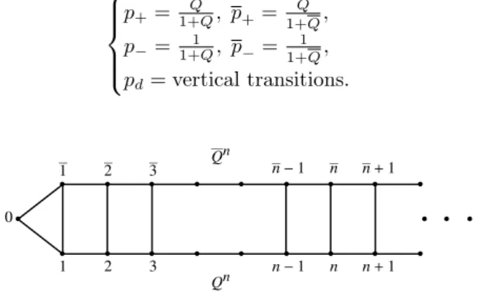
7.3. A 2D LATTICE
LetG= (V, E, c)the graph in Figure 7.6. FixQ, Q >1, and set the conductance as
an:=cn−1,n=Qn,
an:=cn−1,n=Q n
for alln∈Z+. We get the set of transition probabilities as follows:
p+=1+QQ, p+=
Q
1+Q,
p−= 1+1Q, p− =1+1Q, pd=vertical transitions.
0
1 2 3 n-1 n n+1
Qn
1 2 3 Q n-1 n n+1
n
Fig. 7.6. Conductance:cn−1,n=Qn andcn−1,n=Q n
7.4. A PARSEVAL FRAME THAT IS NOT AN ONB INHE
Letc01, c02, c12be positive constants, and assign conductances on the three edges (see Figure 7.7) in the triangle network.
0
1 2
c01 c02
c12
Fig. 7.7. The set{vxy: (xy)∈E}is not orthogonal
We show that wij =√eijvij,i < j, in the cyclic order is a Parseval frame but not
an ONB inHE.
Note the corresponding Laplacian ∆ (= ∆c)has the following matrix
representa-tion:
M :=
−c(0)c01 −c(1)c01 −−cc0212
−c02 −c12 c(2)
The dipolesvxy: (xy)∈E(ori) as 3-D vectors are the solutions to the equation
∆vxy=δx−δy.
Hence,
M v01=
1 −1 0tr,
M v02=1 0 −1
tr
,
M v12=0 1 −1
tr
.
We check directly eq. (3.17) holds, and sovxy: (xy)∈E(ori) is not orthonormal.
For example, we have
v01=
c12
c01c02+c01c12+c02c12
,−c c02
01c02+c01c12+c02c12
,0
tr
and
c01(v01(0)−v01(1)) = c01(c12+c02)
c01c02+c01c12+c02c12
<1;
see (3.17). Hence the voltage drop across (01)is strictly smaller then the(01) resis-tance, i.e.,
v01(0)−v01(1)<
1 c01
=Res(01).
In this example, the Parseval frame from Lemma 3.2 is
w01=√c01v01=
√c
01c12
c01c02+c01c12+c02c12
,−
√c
01c02
c01c02+c01c12+c02c12
,0
tr
,
w12=√c12v12=
0,
√c
12c02
c01c02+c01c12+c02c12
,−
√c
12c01
c01c02+c01c12+c02c12
tr
,
w20=√c20v20=
−√c20c12
c01c02+c01c12+c02c12
,0,
√c
20c01
c01c02+c01c12+c02c12
tr
.
Remark 7.14. The dipole vxy is unique in HE as an equivalence class, not a
function on V. Note kerM = harmonic functions = constant (see (7.32)), and so
vxy+const=vxy inHE. Thus, the above frame vectors have non-unique
representa-tions as funcrepresenta-tions onV. Also see Remark 3.5.
Introduce the vector system of conductance as follows:
e
c1= (c01, c01, c02),
e
c2= (c02, c12, c12),
e
We arrive at the following formula for the spectrum of the system(V, E, c,∆), where
(V, E)is the triangle in Figure 7.7.
λ1= 0,
λ2=trec0−
q
kec0k2− hec1,ec2i,
λ3=trec0+
q
kec0k2− hec1,ec2i, and so the spectral gap
λ3−λ2= 2
q
kec0k2− hec1,ec2i is a function of the coherence forec1 andec2.
8. OPEN PROBLEMS
LetG= (V, E, c)be a graph, with verticesV, edgesE, and conductancec;V is count-able infinite. The graph-Laplacian ∆ is essentially selfadjoint as an l2(V)-operator, but not as a HE-operator. It is known that ∆, as a HE-operator, has deficiency indices(m, m),m >0, when the conductance functionc is of exponential growth.
1. Compare the deficiency indices of ∆ (in HE) for various cases: V = Zd,
d= 1,2,3, . . .; nearest neighbor. If d = 1 must the indices then be (m, m) with
m= 0or 1? Are there examples withm= 2 in any of the classes of examples? 2. What is the spectral representation of the Friedrichs extension ∆F ri as a
HE-operator? Find theHE projection valued measure.
3. Find the spectrum of the transition operator P, considered as an operator in
l2(V,ec). When is there point-spectrum? If so, what are the two top eigenvalues? What is the connection between this spectrum (the spectrum ofP), and the spec-trum of ∆F ri in HE, and of ∆inl2(V)?
4. It is not known whether or not the transition operatorPis bounded as an operator of HE into itself.
Acknowledgments
The co-authors thank the following for enlightening discussions: Professors Sergii Bezuglyi, Dorin Dutkay, Paul Muhly, Myung-Sin Song, Wayne Polyzou, Gestur Olafsson, Robert Niedzialomski, Keri Kornelson, and members in the Math Physics seminar at the University of Iowa.
REFERENCES