http://dx.doi.org/10.1590/S1982-21702014000300035
OUTLIERS DETECTION BY RANSAC ALGORITHM IN THE
TRANSFORMATION OF 2D COORDINATE FRAMES
Detecção de valores aberrantes com o uso de algoritmo RANSAC na transformação de coordenadas rectangulares.
JOANNA JANICKA JACEK RAPINSKI
University of Warmia and Mazury in Olsztyn, Institute of Geodesy ul. Oczapowskiego 1, 10-719 Olsztyn
[email protected]; [email protected]
ABSTRACT
Over the years there have been a number of different computational methods that allow for the identification of outliers. Methods for robust estimation are known in the set of M-estimates methods (derived from the method of Maximum Likelihood Estimation) or in the set of R-estimation methods (robust estimation based on the application of some rank test). There are also algorithms that are not classified in any of these groups but these methods are also resistant to gross errors, for example, in M-split estimation. Another proposal, which can be used to detect outliers in the process of transformation of coordinates, where the coordinates of some points may be affected by gross errors, can be a method called RANSAC algorithm (Random Sample and Consensus). The authors present a study that was performed in the process of 2D transformation parameter estimation using RANSAC algorithm to detect points that have coordinates with outliers. The calculations were performed in three scenarios on the real geodetic network. Selected coordinates were burdened with simulated values of errors to confirm the efficiency of the proposed method.
Keywords: Coordinate Transformation; RANSAC; Parameter Estimation.
RESUMO
(derivados do método Maximum Likelyhood Estimation) ou R- estimações. Outros métodos são também conhecidos que não se incluem a nenhum desses grupos, e que também, mostram resistência aos erros grossos, por exemplo, Msplit estimação. A proposta neste artigo, que pode se aplicar ao processo de transformação de coordenadas, quando as coordenadas de alguns de pontos podem estar contaminadas por erros grosseiros, é o método denominado de RANSAC algoritmo (Random Sample and Consensus). Os autores apresentam a possibilidade da utilização deste método numérico para a detecção erros grosseiros nas coordenadas de pontos utilizados na estimação dos parâmetros de transformação. Experimentos foram realizados com três cenários de erros nos dados utilizando uma rede real de pontos. Os resultados obtidos nos experimentos realizados com dados simulados foram animadores e confirmam a eficiência do algoritmo proposto grosseiros para verificar a eficácia do método proposto.
Palavras-chave: Transformação de Coordenadas, RANSAC, Estimação de
Parâmetros.
1. INTRODUCTION
general RANSAC algorithm is described. Section 3 presents implementation of this algorithm for coordinate transformation. Section 4 shows the results of tests of the above procedure using a data set with various numbers of outliers.
2 . RANSAC ALGORITHM
The RANSAC algorithm was first introduced by Fischler and Bolles in 1981 as a method to estimate the parameters of a certain model, starting from a set of data contaminated by large amounts of outliers. It is an iterative, non-deterministic algorithm which uses least-squares to estimate model parameters. The basic premise of RANSAC is the presence in the data set of both observations that fit the model (inliers) and those which differ from the values (outliers). The sources of data that do not fit into the model are gross errors (measurement errors), noise or other disturbances. The input data of the algorithm are: a set of data and a mathematical model that will be matched to the data set. The advantage of this method is that the percentage of outliers which can be handed by RANSAC can be larger than 50% of the entire data set (MURRAY & TORR, 1997). Such a percentage, known also as the “breakdown points”, is commonly assumed to be the practical limit for many other commonly-used techniques for parameter estimation (such as a robust estimation method, for example, for the Huber, Hampel and Danish methods).
The RANSAC algorithm is essentially composed of two steps that are repeated in an iterative process:
1. Hypothesis, 2. Tests.
Apriori information, which is used in the process of fitting the model includes: 1. Minimum number of points (observations) required to fit the model; 2. Minimum number of iterations;
3. Parameter (md) determining the threshold that splits the inliers from outliers
in the process of hypothetical model testing;
In the testing step, RANSAC iteratively checks which entire dataset are consistent with the hypothetical model. This the value of the parameter md specifying the maximum distanc
a hypothetical model. If it fits the criterion of md, the point is tr
hypothetical inlier. The minimum percentage of observation correct data in the whole data set must be also defined by us model can be regarded as properly defined if 80% of the observ are not burdened with outliers). The estimated model is correct number of points that have been classified as correct observatio set of observations which is selected from the entire dataset is set (CS). Defining iteration as a single process of random sele testing, the number of iterations is determined by the following
(
q
)
=
T
iter−
1
log
log
ε
where:ε – probability of incorrect identification of the model,
q – is calculated based on the following equation:
q = (Ni/N)k
in which: Ni – the number of points that belong to the consensus
N – the total number of points,
k – minimal number of data that are necessary to clearly define
If we want to obtain an error-free selection of points (MS 1-ε, we need to perform at least T iterations.
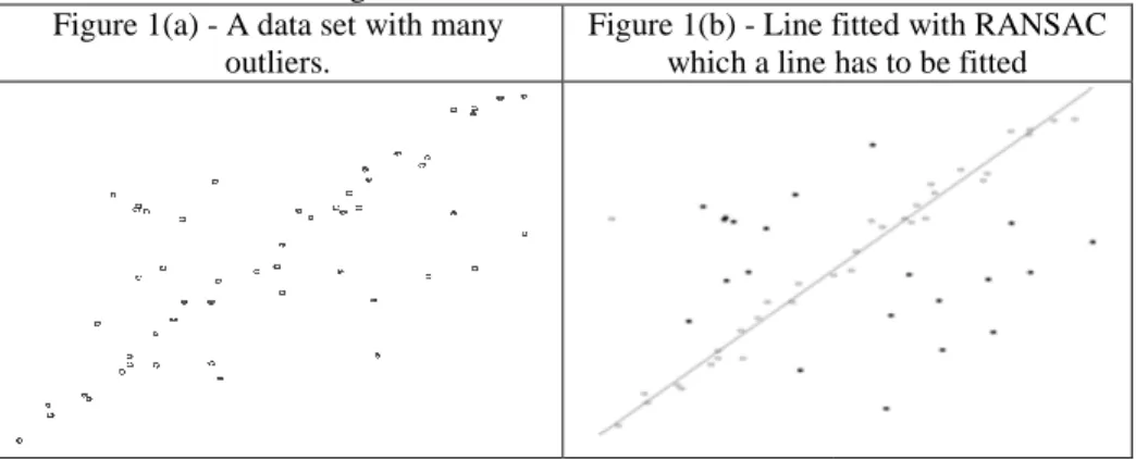
Figure 1 depicts an example of the application of RANS parameters. The data set containing correct observations (inlie burdened with gross errors (outliers) is shown in Figure 1.
Figure 1 – The data set observations. Figure 1(a) - A data set with many
outliers.
Figure 1(b) - Line f which a line h
ch observations of the is requires determining nce from a test point to s treated as just another tions that must be the user (for example, the ervations are those that ect if it has a sufficient tions (inliers). The best is called the consensus election of MSS and fit ng formula:
(1)
(2)
sus set,
ne the model.
SS) with a probability
NSAC to estimate line liers) and observations
Figure 1(a) presents the entire input data set, from which the correct observations describing a straight line are selected. Figure 1(b) shows the line that is based on the correct observation (inliers) selected by the RANSAC algorithm and the solid dots are the outliers that do not fit the model.
3. RANSAC APPLICATION IN TRANSFORMATION PARAMETER ESTIMATION
The RANSAC algorithm described in the previous section can be used in transformation parameter estimation. It is particularly recommended if the results of standard least squares estimation are not satisfactory. It can imply that outliers are present in the set of reference points. To confirm the effectiveness of the proposed method, the Helmert transformation was adopted. Traditionally, determination of transformation parameters is performed by the least-squares method using all available points in a single computational process. Unfortunately, since the least squares method is not a robust method, this method is not immune to outliers. It means that if, for any reason, one or more of the reference point coordinates is not correct, the transformation parameters calculated using least squares will be estimated with this error. Such observations must be eliminated from the data set before performing least square estimation of coordinate transformation parameters. In this paper, the RANSAC algorithm for estimation of coordinate transformation parameters is proposed to complete this task. The RANSAC algorithm used during the parameter estimation process allows selecting only those points that are not outliers to be used in the estimation. In each step of this algorithm, the transformation parameters are still estimated by the least squares method. The greatest benefit of this approach is that the percentage of outliers can be larger than 50% of the entire set of reference points.
The RANSAC transformation is an iterative process and is described as follows:
1. Helmert transformation in two-dimensional space is a four-parameter transformation. Thus, the minimum number of reference points is two. In the first step, two reference points are randomly selected from the entire set of reference points and the transformation parameters are calculated by solving a set of four linear equations. This is the step of creation of the hypothetical model.
2. The next step is the transformation of reference points coordinate from one Cartesian coordinate system to another (e.g. old local Cartesian coordinate system to the national 2000 coordinate system used in Poland) with the hypothetical transformation parameters (from the first step, on the basis of the hypothetical model).
3. Definition of the parameter md, the minimum number of iterations and the
4. Calculation of Euclidean distances to each point from the points transformed using a hypothetical model and testing conditions: if d < md then the point is added to the minimal set of reference points described in the first step, then if the number of inliers is sufficient (e.g. min 80% of the entire set of total points).
5. If all conditions from step 4 are satisfied, the iteration process is finished (Fig.2). The Consensus Set (CS) is then defined and based on it, the transformation parameters are re-estimated by the least-squares method. If conditions are not fulfilled, then RANSAC algorithm once again selects the minimum number of points to define a hypothetical model and the procedure 1-4 is repeated.
6. The final step is the transformation of coordinates from one geodetic system to another using the CS model parameters.
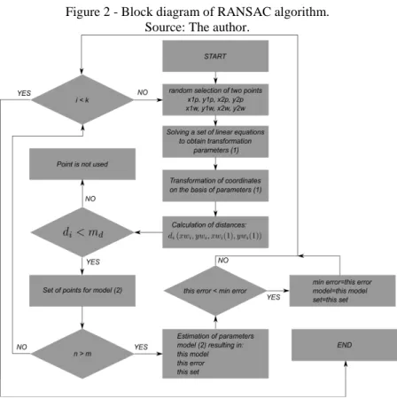
Figure 2 presents the block diagram of the RANSAC transformation.
Figure 2 - Block diagram of RANSAC algorithm. Source: The author.
coordinates in primary coordinate system, x1w, y1w, x2w, y2w are coordinates in the secondary coordinate system.
4. EXAMPLE
An analysis performed using real data (i.e., a horizontal geodetic network) confirmed the effectiveness of the proposed algorithm. This object (named JAROCIN) is a horizontal geodetic network, which includes 158 points. The coordinates of these points are defined in the local coordinate system and in the Polish Coordinate System “2000”, where 54 of them are reference points. The “2000” reference frame was introduced in Poland in 2000 as a new national reference frame after the ETRF (European Terrestrial Reference Frame) was adopted. Since the previous reference frame in Poland was based on the Krassowski ellipsoid, it was necessary to define a new system and create a new database of control networks in the “2000” reference frame. There are two ways in which this task can be accomplished: re-surveying of the entire networks and new adjustment in the 2000 frame and transformation of coordinates from the previous reference frames (either “1965” or local).
Re-surveying is preferable in the case of the high order networks. Transformation was allowed in the case of local coordinate frames and lower order networks. In many cases, a problem with outliers in the coordinates of reference points occurred in the transformation process. Reference points (points used to calculate transformation parameters), burdened with unidentified outliers had a significant influence on transformation results. Therefore, it was necessary to find a way to automatically identify outliers among reference point coordinates. The JAROCIN network was re-measured and re-adjusted in 2007 in “2000” reference frame. Since the mean error of coordinates was smaller than 2 cm, these coordinates were considered as error free for the purpose of the RANSAC transformation method testing. In the rest of the article this coordinates will be called “catalogue coordinates”.
The transformations were performed in three scenarios with different numbers of reference points burdened with gross errors (13, 27 and 45 outliers respectively) and different value of these errors. The artificial errors were added to both X and Y coordinates. Number of iterations performed for each scenario with respect to the ε parameter is presented in Table 1.
Table 1 - Number of RANSAC iterations. Scenario Number of
outliers
1-ε
90% 95% 99.7%
1 13 3 3 7
2 27 8 10 20
The first scenario assumed that 24% (13 out of 54) of the reference point coordinates included outliers with a magnitude from 0.15-0.30 m. The purpose of the RANSAC algorithm in the process of coordinate transformations is to use only the correct observation. Outliers will not be taken during the estimation of the transformation parameters. The RANSAC algorithm should choose 41 points that are not burdened with gross errors and calculate the correct transformation parameters. Figure 3 and 4 present the histogram of the residuals X and Y obtained in the first scenario.
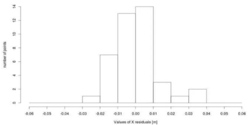
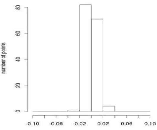
Figure 3 - Histogram of the 41 points X residual obtained in the first scenario.
Figure 3 presents a histogram of the X residuals obtained in the first scenario. The values of these residuals are between -0.03 to 0.04 m.
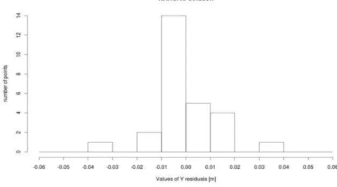
The Figure 4 shows the histogram of the Y residuals obtained in the first scenario. In this figure, the values of these residuals are also between -0.03 to 0.04 m.
The RANSAC algorithm identified all outliers and the transformation parameters were computed using 41 correct points. The resulting coordinates obtained from RANSAC transformation were compared with catalogue coordinates and the differences between them were calculated. The resulting coordinate differences are presented as histograms in Figure 5 and 6.
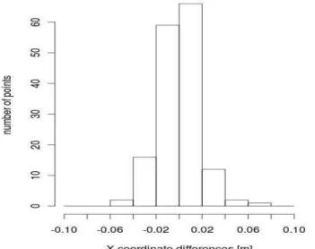
Figure 5 - Histogram of the differences between X coordinates after RANSAC transformation and catalogue values in the first scenario.
The Figure 5 presents the histogram of the X coordinate differences obtained in the first scenario. The values of these differences are between -0.06 to 0.08 m. However, more than 80% of the differences are less then ±0.02m.
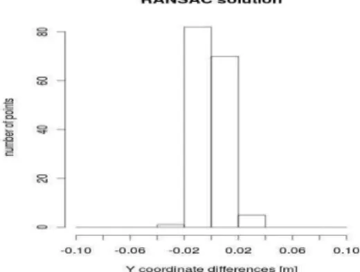
Figure 6 presents the histogram of the Y coordinate differences obtained in the first scenario. The values of these differences are between -0.04 to 0.04 m.
Figure 6 - Histogram of the differences between Y coordinates after RANSAC transformation and catalogue values in the first scenario.
The calculation in the second scenario performed on the same dataset JAROCIN, which includes 158 points and 54 of them are reference points. In this scenario the gross errors of magnitude of 0.15 to 0.30 m were added to the X and Y coordinates of 50% of reference points (27 out of 54 reference points). The RANSAC algorithm should choose 27 points that are not burdened with gross errors and calculate the correct transformation parameters Then the transformation parameters were estimated and the transformation was performed. The values of the residuals obtained in this scenario are shown in Figures 7 and 8.
The Figure 7 presents the histogram of X residuals obtained in the second scenario. In this scenario, the values of the residuals are between -0.03 and 0.04 m.
Figure 8 - Histogram of the 27 points Y residual obtained in the second scenario.
In the Figure 8, the histogram of 27 point residuals is shown. Based on this, it can be determined that more than 90% of the residuals are less than +-0.02 m.
In the second scenario the RANSAC algorithm again identified all outliers and the transformation parameters were computed using 27 correct points. Then the transformation of 158 points from local coordinate system to the Polish Coordinate System “2000” was performed. The histograms of the differences between coordinates after transformation and catalogue values are shown in Figures 9 and 10.
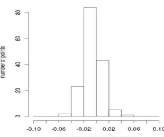
Figure 9 presents the histogram of the X coordinate differences obtained in the second scenario. The values of these differences are between -0.06 and 0.06 m. However, almost 80% of the differences are less than ± 0.02m.
Figure 10 - Histograms of the differences between coordinates Y after RANSAC transformation and catalogue values in the second scenario.
Figure 10 presents the histogram of the Y coordinate differences obtained in the second scenario. The values of these differences are between -0.04 to 0.04 m but more than 90% of the differences are less than ± 0.02m.
From Figures 9 and 10 it is clear that all of the coordinate differences are much smaller than the value of gross errors. It shows that the RANSAC algorithm again prevented outliers from being used in transformation parameters estimation.
The calculation in the third scenario was performed on the same data set JAROCIN. In this scenario the gross errors of magnitude of 0.15 to 0.30 m were added to the X and Y coordinates of 83% of reference points (45 out of 54 reference points). The RANSAC algorithm should choose 9 points that are not burdened with gross errors and calculate the correct transformation parameters. The residuals, calculated to the nine correct reference point coordinates, are presented in Figures 11 and 12.
The Figure 11 presents the histogram of X residuals obtained in the third scenario. In this scenario, the values of the residuals are between -0.01 and 0.02 m.
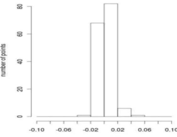
Figure 12 - Histogram of the 9 point residuals Y obtained in the third scenario.
The Figure 12 presents the histogram of Y residuals obtained in the third scenario. The values of the residuals are about ± 0.01 m.
The resulting coordinate differences are presented as histograms in Figures 13 and 14.
In the Figure 13, the histogram of the X coordinate differences obtained in the third scenario is presented. The values of these differences are between -0.06 and 0.06 m as in the second scenario. The results of the transformation are almost the same in those two scenarios.
Figure 14 - Histograms of the differences between Y coordinates after RANSAC transformation and catalogue values in the third scenario.
Figure 14 shows the histogram of the Y coordinate differences obtained in the third scenario. The differences are similar to the Y coordinate differences in the second scenario and are between -0.04 and 0.06 m.
In this scenario, the coordinates of 45 points are contaminated by outliers. Thus, only 9 out of 54 points are not burdened with gross errors. In this case, traditionally used robust estimation methods would not give the correct result. These methods would recognize those nine correct points as outliers and 45 bad points as correct points. RANSAC transformation correctly identified 9 points (inliers) and the transformation parameters were estimated based on them.
Analyzing the coordinate differences obtained in all scenarios of the calculations, it can be seen that the X coordinate differences are slightly larger than Y coordinate differences. Since point coordinates used in this experiment were obtained from the GNSS survey (for a second frame) this might be the influence of some surveying errors (due to bad satellite geometry or horizon obstructions at some points). However, it had no effect on the calculation results.
5. DISCUSSIONS AND CONCLUSIONS
case with 24% of points contaminated with outliers and continued with a 50% of outliers up to a very high number of 83% of points contaminated with outliers.
In each variant, the desired results of the calculations were achieved. The algorithm was able to find a correct solution and to eliminate outliers from estimation process. Therefore, the effectiveness of RANSAC algorithm applied to estimation of coordinate transformation parameters is confirmed. The main goal of the study was to confirm the possibility to properly estimate coordinate transformation parameters, when the total number of points burdened with errors is greater than 50%. Calculations performed in the second and third variants prove the effectiveness of the proposed algorithm, with the number of observations burdened with errors at the level of 83%. In all three scenarios both residuals and calculated distances between catalogue coordinates and coordinates after transformation were at the level of random observation error. The number of required iterations increased with the number of outliers in the data set. To assure for 99.7% that in the third scenario the algorithm will select two points that are not outliers 206 iterations were required (Table 1).
Despite the advantages of this method, it has some flows. It is not an efficient method from a computational point of view. Number of iterations increases with the number of outliers in the data set and with required probability of successful selection of two inliers. It requires much iterations and many operations which sometimes (especially in the case of large sets) take a longer time than the standard procedure. There is also a risk that the algorithm will not select the proper two points for the best solution (which depends on the a priori selection of ε parameter). Therefore, an insightful analysis of results is required.
BIBLIOGRAPHICAL REFERENCES
CHOI, S.; KIM, T.; YU, W. Performance Evaluation of RANSAC Family.
Proceedings of the British Machine Vision Conference (BMVC). p. 1-12 ,
2009.
DUCHNOWSKI, R., Robustness of strategy for testing leveling mark stability based on rank tests. Survey Review. Vol 43(323), pp. 687–699, 2011
FISCHLER, M., BOLLES, R., Random Sample Consensus: A Paradigm for Model Fitting with Applications to Image Analysis and Automated Cartography.
Communications of the ACM. Vol 6(24), pp. 381–395, 1981.
GRUBBS, F., Procedures for detecting outlying observations in samples.
Technometrics. Vol. 11, No. 1(Feb., 1969), pp. 1-21, 1969
HUBER, P. J., Robust estimation of a location parameter, Annals of Mathematical
Statistics, (1), pp. 73–101, 1964
ISACK, H., BOYKOV Y., Energy-based Geometric Multi-Model Fitting. International Journal of Computer Vision. 97(2): 1: 23–147, 2012
JANICKA, J., RAPINSKI, J., M-split transformation of coordinates. Survey
JANICKA, J., Transformation of coordinates with robust estimation and modified Hausbrandt correction. Environmental engineering, (III), pp. 1330–1334, 2011 MURRAY, D.W., TORR, P.H.S., The Development and Comparison of Robust
Methods for Estimating the Fundamental Matrix. International Journal of
Computer Vision, Vol 24, no 3, pp. 271-300, 1997
WISNIEWSKI, Z., Estimation of parameters in a split functional model of geodetic observations. Journal of Geodesy, (83), pp. 105–120, 2008