Roberto Jose Luna Olivares
A convolutional and machine learning
approach
PALM TREE IMAGE CLASSIFICATION
A convolutional neural network and machine learning approachDissertation supervised by
Joel Dinis Baptista Ferreira da Silva, PhD Instituto Superior de Estatística e Gestão de Informação,
Universidade Nova de Lisboa Lisbon, Portugal
Dissertation co-supervised by Pedro da Costa Brito Cabral, PhD
Instituto Superior de Estatística e Gestão de Informação, Universidade Nova de Lisboa
Lisbon, Portugal
Dissertation co-supervised by Ignacio Guerrero, PhD
Institute of New Imaging Technologies, Universitat Jaume I
Castellón de la Plana, Spain
I would like to thanks my supervisor Joel Silva, for sharing his knowledge, encour-agement and guidance, made this research project enjoyable and fulfilling. To my co - supervisors Pedro Cabral and Ignacio Guerrero for their feedback and constructive
criticism.
Thanks for the effort to all the professor that helped through the master programs. Special thanks to professors Marco Painho and Christoph Brox for their guidance and advice for the duration of the program.To all my classmate that became my family during this period. To the Erasmus Mundus program for giving me the opportunity to complete this master programs and have an unforgettable experience.
I don’t believe it. Prove it to me and I still won’t believe it
A convolutional and machine learning approach
Abstract
Convolutional neural networks have proven to excel at image classification tasks, do to this they have being incorporated into the remote sensing field, initial hurdles in their application like the need for large data sets or heavy computational burden, have being solve with several approaches. In this paper the transfer learning approach is tested for classification of a very high resolution images of a palm oil plantation. This approach uses a pre trained convolutional neural network to extract features from an image, and label them with the aid of machine learning models. The results presented in this study show that the features extracted are a viable option for image classification with the aid of machine learning models. An overall accuracy of 97% in image classification was obtained with the support vector machine model.
KEYWORDS
Convolutional Neural Network Machine Learning
Unnamed Aerial Vehicle Image Classification Transfer Learning OverFeat
GIS - Geographical Information Systems
GEOBIA - Geographic Object-Based Image Analysis CNN - Convolutional Neural Network
UAV - Unmanned Aerial Vehicle FVP - First Person View
RC - Remote Control
CMOS - Complementary Metal-Oxide Semiconductor CHDK - Canon Hack Development Kit
RF - Random Forest LR - Logistic Regression DT - Decision Tree
GBC - Gradient Boost Classifier KNN - K nearest neighbor SVM - Support Vector Machine TP - True Positives
TN - True Negatives FP - False Positives FN - False Negatives
I N D E X O F T H E T E X T
INDEX OF FIGURES x
INDEX OF TABLES xi
1 Introduction 1
1.1 An overview of the work . . . 1
1.2 Aim and Objectives . . . 3
1.3 Document organization . . . 3
2 Literature review 4 2.1 Remote sensing and UAV applications . . . 4
2.1.1 Remote sensing . . . 4
2.1.2 UAV applications . . . 5
2.2 Machine learning techniques in Remote Sensing. . . 6
2.3 Convolutional neural-networks . . . 7
2.4 Application of CNN in Remote Sensing . . . 9
2.5 Fundamentals of CNN . . . 10
2.6 OverFeat . . . 11
3 Data and Methods 13 3.1 Description of study area . . . 13
3.2 UAV System . . . 13 3.3 Aerial survey . . . 15 3.4 Data set . . . 15 3.5 Methodology . . . 17 3.5.1 Tools . . . 17 3.6 Data Preprocessing . . . 18
3.7 OverFeatand Feature Extraction . . . 19
3.8 Machine Learning Models . . . 19
3.9 Visualization . . . 20
3.10 Accuracy assessment . . . 20
4.1 Result overview . . . 21
4.2 Image preprocessing . . . 21
4.3 Feature extraction with OverFeat . . . 22
4.4 Machine learning models classification results . . . 23
4.4.1 SVM classification results . . . 25
4.5 Image Classification . . . 26
5 Discussion and Conclusion 31 5.1 Discussion . . . 31
5.2 Conclusion . . . 34
Bibliographic References 35 I Annex 42 I.1 Example of features extracted using OverFeat . . . 42
I.2 Image classification results . . . 42
I.3 ROC graphs . . . 43
I.4 Confusion matrix . . . 45
II Annex 2 47 II.1 Cropping Images . . . 48
II.2 Extracting features with Overfeat . . . 48
II.3 Machine learning Models . . . 50
II.4 Fine tuning Machine learning Models . . . 51
I N D E X O F F I G U R E S
2.1 Artificial neural network architecture. . . 8
2.2 Architecture of a Convolutional Neural Nework . . . 11
3.1 Study area in Loma de Mico, East Nicaragua . . . 14
3.2 Fixed wing UAV model Skywalker 1800 used for aerial survey . . . 15
3.3 Flowchart depicting the methodology, yellow shapes represent beginning and finish product, blue intermediate results, green process, red input data 17 3.4 Example of original image and cropped image. . . 18
4.1 Examples of objects in the tiles. . . 22
4.2 Overall accuracy and standard deviation of models . . . 23
4.3 SVM classifier ROC curve . . . 27
4.4 Image classification results . . . 28
4.5 Examples of tiles classified as False Positives . . . 29
4.6 Examples of tiles classified as False Negatives . . . 30
I.1 Image classification results . . . 43
4.1 Cropped tiles and labels given based on presence of palms . . . 21
4.2 Accuracy assessment of Classification models . . . 24
4.3 Confusion matrix DT . . . 24
4.4 Confusion matrix GBC . . . 24
4.5 Confusion matrix SVM . . . 25
4.6 Classification results from SVM model for each image . . . 26
I.1 Confusion matrix SVM . . . 45
I.2 Confusion matrix DT . . . 45
I.3 Confusion matrix LR . . . 45
I.4 Confusion matrix GBC . . . 45
I.5 Confusion matrix KNN . . . 46
C
h
a
p
t
e
r
1
I n t r o d u c t i o n
1.1 An overview of the work
Agriculture is one of the most important economical activities in the world and spe-cially in developing countries. Nonetheless current agro-industrial means of produc-tion carry a heavy impact on the environment, specially palm oil Elaeis guineensis plantations. Palm oil has become a very popular crop due it’s high demand since it’s used in a wide range of products in our society from food, cosmetics, pharmaceutic,
bio fuels and its demand has being steadily increasing since 1992 Sumathi et al. (2008).
But this high demands also implies land cover changes, and in the case of palm this is
happening in an alarming rate Fitzherbert et al. (2008), such that there’s international
pressure to stop the expansion of new palm tree plantations and effectively manage current croplands. To better manage resources a paradigm shift in the means of pro-duction is required, this is a difficult task but with help of technological advancement it can be achieved. Remote sensing techniques are widely applied in diverse fields, but
one of the stand out is agriculture Atzberger (2013). Several techniques have being
applied with great results with the goal of achieving a better management of resources and reducing the environmental impacts of agriculture. In this context this study will focus on image classification of a palm oil plantation, with the view of helping better manage crop lands by providing information of areas with palms. The method will be based on the use of very high resolution images obtained from an Unnamed Aerial vehicle (UAV), a convolutional neural network (CNN), to extract data from the images and machine learning (ML) algorithms to classify the data.
CNN are fast evolving field and have proven to excel at image recognition task Girshick (2015), Krizhevsky et al. (2012), Long et al. (2015), Ren et al. (2015), and
training, in the sense that it needs to see large amounts of labeled data Krizhevsky
et al. (2012). The remote sensing community have taken great interest of the great
performance of them in object classification task and have tried to apply them in a remote sensing context. Nevertheless this methods has some drawbacks, as mentioned before they require large amounts of labeled data to learn to detect objects, training one from scratch involves heavy computational burden and time, nonetheless some studies have proven viable methodology to overcome these hurdles. Fine tuning a network is one of the option, this requires knowledge about the architecture of the network, the data that it will be analyzing and several analysis of the data fo obtaining
a model that performs the required task, Nogueira et al. (2017) tested this approach
obtaining good results. Another option is transfer learning, this method relies on using the capacities of CNN to extract features from image and later using this data coupled
with machine learning models to classify or label the data, Sharif Razavian et al. (2014)
proved in his study that this "off the shelf CNN" approach yields results that compete with the state of the art methods, this had made these methods popular among remote sensing applications.
Several studies have focused on the use of transfer learning for image classification,
but mainly focused on the use of satellite imagery Hu et al. (2015) and Penatti et al.
(2015), but not as much in the case of very high resolution imagery obtained from an
UAV Zortea et al. (2018). This research can help narrow the gap and serve as reference
for how CNN interact with very high resolution images. Based on the previous studies that used transfer learning, good results should be expected, the features extracted with the CNN will be able to differentiate palms in the images.
Therefore this research seeks to determine if features extracted from very high resolution UAV imagery, using a pre trained CNN, can translate to solving an image classification scenario. In this case the classification will be done using ML models and determining which one performs the best for this specific case.
To test this hypothesis, the pre trained OverFeat network Sermanet et al. (2013),
will be used as feature extractor, and to classify the features six machine learning models will be employed, and their accuracy will be assessed, the best model for this specific case will be used to classify the images of the data set.
This research will provide data about how viable is to use a pre trained CNN and transfer learning approach for image classification, in the context of using a data set consisting of very high resolution images obtained with an UAV. On the other hand this study will provide a method for image classification that can hopefully serve as a base and further developed to produce an efficient resource management for palm tree plantations.
1 . 2 . A I M A N D O B J E C T I V E S
1.2 Aim and Objectives
The main aim of this research is to classify if images from the data set contain palms. Objectives
• Evaluate if the features extracted by OverFeat transfer well enough to perform classification of very high resolution images.
• Evaluate several machine learning models for classifying features extracted from OverFeat.
• Use the best machine learning model to classify the images in the data set.
1.3 Document organization
The document is organized into five sections. First chapter includes an introduction with an overview about the topic and context in which this research was developed, as well the objectives. Second chapter has theoretical concepts that serve as basis for the completion of this study. Chapter three is a description of the methodology and tools use, chapter four presents and describes results of the study. Final chapter is the discussion of the results and conclusion. Annex I contains results that were not showed on chapter 4 and Annex II contains programming scripts that were used in this study.
C
h
a
p
t
2
L i t e r a t u r e r e v i e w
This chapter will discuss applications of UAV technologies in the remote sensing field with special interest in previous work linked with image classification using CNN. The second part will about theoretical approaches and application of machine learning models and CNN in remote sensing for image classification.
2.1 Remote sensing and UAV applications
2.1.1 Remote sensing
In a general context remote sensing is the act of acquiring data from an object,
phe-nomena or geographical space with out direct interactionLillesand et al. (2014). The
year 1972 is a benchmark for civilian remote sensing with the launch of Landsat 1, this system set the basis and norms for multi spectral sensor technologies Blaschke
et al. (2014). From this point on the field has been in a constant state of evolution
pushed by technological progress and a growing body of research Atzberger (2013),
Colomina and Molina (2014), Navalgund et al. (2007), and Pajares (2015), to the point
of becoming a staple in many and diverse applications Basse et al. (2016), Hedley et al.
(2016), Masini et al. (2018), Megahed et al. (2015), and Richter et al. (2016). The
success of remote sensing allowed for new technologies to be incorporated, such is the case of unmanned aerial vehicles (UAV).
There are many definitions for UAV, for example, the international civil aviation organization of the United nations (ICAO), defines it as: A set of configurable elements consisting of a remotely-piloted aircraft, its associated remote pilot station(s), the re-quired command and control links and any other system elements as may be rere-quired, at any point during flight operation."International Civil Aviation Organization (2011). This definition is broad and can encompass a wide range of system, from military grade
2 . 1 . R E M O T E S E N S I N G A N D UAV A P P L I CAT I O N S
equipment to small radio control aircraft, therefore this review will focus on the
defi-nition proposed by Watts et al. (2012), as it fits into the type of system that was used
for collecting the data for this study. Watts proposed definition considers three main parameters: altitude, endurance and flight capabilities, depending on these character-istics a UAV can fit into an specific category, such as Low Altitude Short-Endurance (LASE) systems. These platforms typically have a payload in the range of 2-5 kg, with a wingspan smaller than 3 meters, up to 2 hours of flight time and can operate in a range of 5 km with a ground station. In other words, this would be considered a “small UAV", and are the systems most commonly used and widespread in research projects Zecha et al. (2013).
Several factors can be attributed to the UAV thriving in remote sensing, technology has played a prominent role with breakthrough in positional and navigation systems
Zecha et al. (2013), miniaturization of hardware and sensors Casagrande et al. (2018)
and Salamí et al. (2014), that made it technically and economically feasible to create
systems capable of autonomously following a flight path and gather remote sensed data. This trend also spread to data processing hardware and software, extracting information became efficient, relatively cheap and accessible to the general public.
Other important factors to be considered are the flexibility a UAV provides regard-ing temporal, spatial and spectral resolution. The modular nature of these systems
allows for seamlessly interchangeable sensors Zecha et al. (2013), as well as the
pos-sibility for selecting the best condition and time for surveying an area Salamí et al.
(2014). This characteristics and flexibility allows this systems to serves as a
comple-ment or even substitute to traditional platforms like space borne or piloted air crafts
Salamí et al. (2014). In some cases UAV is the only viable option for accessing or
obtaining information of remote and dangerous areas for humans Bollard-Breen et al.
(2015) and Everaerts (2008) and finally, depending on the context and scale of the
application, they can be a cheaper alterntive to traditional methods Iizuka et al. (2018)
and Watts et al. (2012).
In conclusion technological advancement made it so, that it’s no longer necessary to have highly trained personnel and equipment to build a UAV, obtain data, process it and extract useful information.
2.1.2 UAV applications
There are many applications for UAV data in remote sensing, cartography
produc-tion is one of the principle examples, Berteška and Ruzgien ˙e (2013) obtained images
and produced digital elevations models (DEM), that fulfill the requirements of
topo-graphical and GIS applications. Researched done by Mesas-Carrascosa et al. (2014)
assessed the quality of orthophotos generated by UAV, the spatial accuracy was eval-uated using techniques employed by mapping agencies, with positive results. A new field where UAVs are gaining traction is air quality measurement, as the review by
Villa et al. (2016) shows a growing interest and applications for measuring air quality, atmospheric composition and air pollutant monitoring.
Geomorphology survey are also being done with the help of UAVs, as proved by
Wang et al. (2016), with soil erosion monitoring in Sancha river basin in Northeast
China. Eltner et al. (2016) presents an overview in the use of high resolution UAV
im-ages for recreating physical objects, this methods have being used in the reconstruction of 3 dimensional objects in various context and research projects.
Vegetation studies have been one of the prominent focus of remote sensing, be it for agricultural or forestry applications. In the field of forest management Mikita et al.
(2016) used aerial and ground photogrammetry for estimating height and diameter
at breast height(DBH), Yuan and Hu (2016) applied random forest models and
object-based classification for identifying pest and monitoring health of forest.
Very high resolution data can be used for single weed mapping, for site specific
plant protection in wheat fields Pflanz et al. (2018), Luna and Lobo (2016) identified
and mapped gaps in sugarcane plantations for optimizing replanting methods, Gago
et al. (2015) analyzed the benefits and gaps of water stress monitoring.
Most of the applications listed above rely on identifying objects, defining their features and boundaries. Many methods have being developed for this purpose, with most of them focused on automating this task. In early stages the focus was on identi-fying large objects do to resolution restrains of sensors. Most of the methods develop where based on statistical analysis of pixels but this meant that underlying spatial
patterns where not considered Casagrande et al. (2018).
With the increasing quality of sensors and the widespread use of UAVs identify-ing smaller objects became feasible, the availability of new data paved the way for a paradigm shift. The core analysis based on statistics were complemented with ob-ject classification, this led to the creation of new concepts, relationships between the
data and methods of analysis. For this concepts Hay and Castilla (2008) proposed the
term geographic object-based image analysis (GEOBIA), they considered to be a a sub-discipline of geographic information science, that focus is creating automated methods for segmenting remotely sensed images into meaningful objects and analyzing their spatial, spectral and temporal characteristics, to create new geographic information
in GIS-ready format Hay and Castilla (2008). This field has benefited from the
devel-opment and advancement of machine learning methods and specially convolutional neural networks (CNN), due to their capacity to solve complex image classification
problems Chen et al. (2018).
2.2 Machine learning techniques in Remote Sensing
Machine learning (ML) techniques are approaches to solving classification and regres-sion problems, they are considered "universal approximators", they can learn the inner workings of a system from a large set of data without prior knowledge Lary et al.
2 . 3 . CO N VO LU T I O N A L N E U R A L- N E T WO R K S
(2016). Being able to model complex systems, capacity of using a wide range of input
and not assuming normal distribution of the data are some of the main reason they have become popular. These characteristics are also common among remote sensed
data Maxwell et al. (2018), therefore this methods have being widely used and applied
by researchers and specialist in the field. Some of the most common ML algorithms are decision trees (DT), sel-organizing map (SOM), random forests (RF), support vec-tor machines (SVM) and artificial neural networks (ANN), the latter two have being
widely applied in the field of geoscience Lary (2010).
Selecting the best algorithm can be a challenging task, as proven by the comparison
done by Maxwell et al. (2018), in which there’s no clear algorithm that constantly
outperforms the rest. This might be caused by deferring methodological approaches and specific characteristics of the data, therefore the best algorithm is case specific and thus it’s recommended that the analysis should include multiple classifiers Lawrence
and Moran (2015).
The scientific literature regarding the use of these methods has being steadily
increasing, Belgiu and Drăguţ (2016) provides and overview of studies using RF
classi-fier, Mountrakis et al. (2011) presents a similar review but for SVM and Maxwell et al.
(2018) compares the accuracy of algorithms in a remote sensing context. Recently
interest and innovation has gravitated towards the development for deep neural net-work, a form of artificial neural netnet-work, that outperform traditional methods Zhang et al. (2016).
Figure 2.2exemplifies a basic artificial neural network architecture, it has three neurons in the input layer, that feed neurons into a hidden layer, which in terms activate the output layer. Deep neural networks are several neural networks stacked together, researches found that adding more layers to the network would increase the accuracy of the model. This has being proven in several studies where convolutional
neiral networks perform image classification task,section 2.3will focus on this models
and their use in remote sensing context.
2.3 Convolutional neural-networks
The first instance of a convolutional neural network is usually credited to the research paper Neocognitron: A Self-organizing Neural Network Model for a Mechanism of Pattern Recognition Unaffected by Shift in Position Fukushima and Miyake (1982), this was a system designed for visual patter recognition and was inspired on the
find-ings of Hubel and Wiesel (1962), on how a cat’s visual cortex is structured and how
it works to identify objects. LeCun et al. (1998) method for recognizing hand written
digits was also an early application of CNN and served as basis for other research and models.
The year 2012 is a benchmark year, as Krizhesvky, Sutskever and Hitton published ImageNet Classification with Deep Convolutional Neural Networks Krizhevsky et al.
Figure 2.1: Artificial neural network architecture Image Source: Glosser.ca (2013)
(2012). Considered to be a seminal work in the field of deep learning, it was the first
instance that a CNN was used for winning the LSVRC (ImageNet Large-Scale Visual Recognition Challenge), a yearly competition in the computer vision field, which re-quires the competitors to develop algorithms that can automatically annotated images
from a data set Russakovsky et al. (2015). The model proposed by Krizhevsky et al.
(2012) called AlexNet, had the lowest error rate in the history of the competition until
that point. The authors explained that the limitations in their model was due to tech-nological constrains as well as amount of data available, and predicted that with more data and technological advancement this type of models would increase in accuracy.
From that point on CNN, were a mainstay in computer vision competitions and their popularity started to permeate into other fields. In the coming years modifica-tions where made to the original model, from fine tuning it’s parameters Zeiler and
Fergus (2013), to simplifying the structure or architecture Simonyan and Zisserman
(2014), to creating new and complex model Szegedy et al. (2015). A tendency was
es-tablished, each new iteration of the CNN model surpassed its predecessor in accuracy.
The fully convolutional network work Long et al. (2015) was another important
benchmark in semantic segmentation, it achieved the goal of assigning each pixel in an image to a class. Parallel to the adjustment made to the CNN architecture and accuracy, other steps were taken into making the process faster and adding features,
such as defining the boundaries of objects Girshick et al. (2014), this method combined
image classification and detection and started a new trend in the field. Subsequent
improvements were made to this approach, in its speed and accuracy Girshick (2015)
and simplifying its structure Ren et al. (2015).
2 . 4 . A P P L I CAT I O N O F C N N I N R E M O T E S E N S I N G
for many applications, including remote sensing. Nevertheless, remote sensed data in general presents some particularities that need to be considered:
• At its core remote sensed data has an important geospatial component that needs to be consider, harnessing these characteristics can led to better analysis. • In general, remotely sensed data comes from wide range of sensors, with different
spectral and spatial resolution, as well as different types of data.
• The large amount of data produced with high temporal resolution is creating a shift towards analysis of time series instead of single scene.
• Remote sensing has traditional approach of detecting and quantifying a phe-nomenon, using models and expert knowledge. On the other hand, deep learning approaches focus on fully automated expert-free knowledge solutions.
2.4 Application of CNN in Remote Sensing
Despite this context remote sensing scientist, have manage to exploit the potential of
deep learning for a varying range of applications. Salberg (2015) proposed a method
for detecting seal pups, from aerial remotely sensed images. The method uses a pre-trained deep convolutional neural network for feature extraction and support vector machine for classification. Results show the method was successful and implies that the methodolgy can be generalized and applied to object recognition in different
sce-narios, but requires further improvements and fine tuning. Chen et al. (2017), used
deep learning techniques to count fruits in a tree, first identifying potential regions of interest (the location of the fruits), then comparing it to ground truth data and finally applying linear regression for estimating a final count, the authors propose using this methodology for plant phenotype identification, counting plants and monitor plant
disease that present visual symptoms. Hung et al. (2014), proposed a method for
ob-taining the best flight altitude for a UAV, for achiving the best classifying performance
for detecting weeds in crop fields, Zhu et al. (2017) provides a review of applications
of CNN, showcasing state of the art methods.
A specific deep learning workflow for detecting and counting palm tree was
pro-posed by Li et al. (2017) their method was tested against manually labeled trees,
showing good results, a limitation they encounter, was the size of their data set. Other method tried to generalize the classification process for different forest types, using a cascade neural network, it showed promising results, but the authors intend to better their method applying a convolutional neural network architecture Tianyang et al. (2018).
2.5 Fundamentals of CNN
A CNN, is a machine learning algorithm, that can learn by analyzing large quantities of data. Its origin stems from artificial neural network models, which are mathematical approximation to how a human brain works. Their general process includes analyzing inputs trough a “neuron” or a layer of mathematical operations and classifying the output depending on its value. This process is achieved by an activation fucntion, this function serves as a threshold for defining the class of the output. For image recognition tasks the input are pixel values.
This models particularity good for image analysis, because they can deal with the large amount of data by reducing their dimension, thus easing the processing burden. They have proven to excel at extracting features from images, performing classification
Krizhevsky et al. (2012) and Szegedy et al. (2015), semantic segmentation Long et al.
(2015) and object detection Girshick et al. (2014), Ren et al. (2015), and Zhu et al.
(2017).
CNN follow a basic structure and its main components can be classified depending on their functions, next a description of the main components is described. This
section is based the lecture notes from Karpathy (2016).
• Convolution layer: This layer receives the input as an array of pixels, each one has three values associated with them, they are width, height and depth, which relates to the number of bands that the image has. This layer transfoms all this information into a function that will describe the pixel, in mathematical terms this is called convolution, thus the name. This operation is performed on the whole image by sliding a filter or kernel. The outputs are values from that summarize each pixel.
• Pooling layer: this part is responsible for reducing the dimension of the con-volved layer, one of the most common methods of doing this is called max pool-ing, which consist on returning the maximum value from each of the convolution operations within a defined window.
• Activation layer: They are in charge of defining which neurons or layers from the network should be activated.
• Fully connected layer: is the layer that is in charge of classifying the features extracted from the previous layers and generates an output. As the name suggest this layers connect all the input layers to the outputs.
In summary when an image is fed to a CNN, the convolutional and pooling layers transform the pixel data, this phase is also called feature extraction, this is when the CNN will recognize geometries in an image, for example identify the structure of a palm tree of a dirt road. The classification of the image is done by the fully connected
2 . 6 . O V E R F E A T
layers, their output is usually a probability score of what the image is.Figure 2.2shows
the architecture of Alexnet Krizhevsky et al. (2012), its structure serve as foundation
to many other models Sermanet et al. (2013) and Zeiler and Fergus (2014).
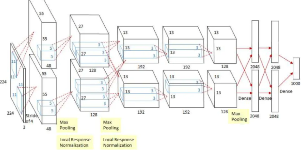
Figure 2.2: Architecture of a Convolutional Neural Nework
Image Source: Krizhevsky et al. (2012)
Despite excelling in image classification tasks, these models have some drawbacks such as the need for large data sets of labeled images as well the time it takes to train a model from scratch, nonetheless there are experience of using pre trained
models as feature extractor with positive results Marmanis et al. (2016), Nogueira
et al. (2017), and Othman et al. (2016). This approach is called transfer learning, it
relies on using a pre trained CNN and removing the fully connected layer (layer that provide classification results), and extracting features using the rest of the architecture
Karpathy (2016). This method provides the mathematical description of geometries
such as edges, curves, size, shapes and angles found in the image. This description are the features from the image and they can be used to train a liner classifier like SVM
Zhang et al. (2015). This approach was also applied in this study, using OverFeat
Sermanet et al. (2013), which is a pre trained CNN that was used as a feature extractor,
this features were later used to train several machine learning classifiers.
2.6 OverFeat
The OverFeat network is based on Alexnet Krizhevsky et al. (2012) with some minor
modifications. It has 6 convolutional layers, they have a varying number of neurons from 96 to 1024, the kernel in these layers vary in size from 3x3 to 7x7 and a max pool-ing layer with kernel size rangpool-ing from 3x3 and 5x5, rounded up by 3 fully connected layers. This model introduced a novel way of increasing classification accuracy by train-ing a CNN to classify and detect objects simultaneously. This framework achieved the best result in the localization task of the 2013 ImageNet Large Scale Visual Recognition Challenge (ILSVRC) and 4th place in the classification task. OverFeat was trained
using ImageNet 2012 training set, which has over a million images spread out in 1000
classes Deng et al. (2009). This data set contains images that are mainly centered and
free from image occlusion and clutter Sharif Razavian et al. (2014).
The best iteration of this model served as base for, OverFeat feature extractor, that was used in this study. There are several instances of the use of OverFeat, Nogueira
et al. (2017) compared three different approaches to using CNN in remote sensing. In
the study they built and train from scratch a CNN, fine tune a pre-trained CNN and
use OverFeatto extract features and classify images. Marmanis et al. (2016) proposed
a two step classification process where they used the pre-trained OverFeat model coupled with another CNN in charge of classifying the features extracted. Sharif
Raza-vian et al. (2014) used OverFeat for various image recognition task, with different
data set obtaining results that compete with highly sophisticated and highly tuned state of the art methods.
In this study the OverFeat network was used as it has yield good results for classification task, also the author provide a version of this model as a ready to use software (https://github.com/sermanet/OverFeat) that can perform feature extraction on our data set with out the need of high computational cost.
C
h
a
p
t
e
r
3
Da t a a n d M e t h o d s
This section will describe the context of the study area, how the data was gather and the most important characteristics.
3.1 Description of study area
The data was gather on September 27 2014, near Loma de Mico village 12°11’ 45.54" N, 83°49’ 48.04"W in the Municipality of Kukra Hill, which is part of the Autonomous region of the Caribbean south coast (RACCs) of Nicaragua (Figure 3.1). Loma de Mico is considered to have a tropical monsoon weather, wet season extends for 10 months, this translates to 2000 - 3000 mm of rain fall. Average temperature ranges from 24 - 27 °C. Rolling hills with slopes between 20 - 30% are staples of the relief, with the highest point rising 192 meter above sea level. The aerial survey was done over a palm tree (Elaeis guineensis) plantation with an area of 45 ha. In it several types of land cover could be distinguished, most prominently present were mature palm trees, palm trees in developing stages, dirt roads, patches of natural forest, grasslands and scatter infrastructure.
3.2 UAV System
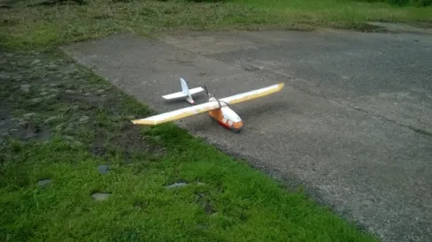
The system used for the aerial survey was a fixed wing glider UAV (Figure 3.2). The airplane is a skywalker model 1800 from 2014, which is originally manufactured as a remote control plane with focus on providing the users first person view (FPV) capabilities. The RC airplane was modified to fit larger payloads (camera, batteries) and with an autopilot, sensors and navigation system making it capable of autonomous
Figure 3.1: Study area in Loma de Mico, East Nicaragua
flight, this was done by the consulting firmEVOLO. Next a detailed description of the
model is given.
The air frame or body was made from EPO (Expanded PolyOlefin) foam, had a total weight of 5 kg, a wingspan of 1800 mm and an endurance of 35 minutes at a speed of 40 km/h. The system used an ArduPilot Mega autopilot APM 2.5, capable of autonomous stabilization and way point navigation, coupled with compass, GPS, barometric pressure sensor and telemetry communication, the system as a whole is capable of completing a pre loaded flight plan autonomously.
The ground control station was a laptop running Mission Planner software version 1.3.10 connected to a radio receiver, this allowed real time communication with the UAV, during the mission it transmitted position (X,Y), height above ground level, yaw, pitch, roll angles, speed and battery levels.
Images were collected using a Canon PowerShot S100 camera (Canon Inc., Tokyo, Japan) this model has a complementary metal-oxide semiconductor (CMOS) sensor size 7.53 x 5.64 mm and an approximate area of 42.5 mm which fits 12,100,000 pixels. Custom firmware CHDK version 1.2 (Canon Hack Development Kit) was setup on the camera. This free software was developed by Canon PoweShot users with the purpose of adding features and enhancing the capabilities of the "point and shoot" camera. In this study it was used to program the camera to take pictures every second by increasing the shutter speed, this would not be possible using the default software provided by the manufacturer.
3 . 3 . A E R I A L S U RV E Y
Figure 3.2: Fixed wing UAV model Skywalker 1800 used for aerial survey
3.3 Aerial survey
The aerial survey started at 15:00 and ended at 15:07 for a total of seven minutes, we assume that atmospheric conditions are uniform in all the images, because during the survey no extreme climatic variance was observed. The flight plan was designed using Mission Planner, taking into consideration characteristics of the camera as well climatic conditions, altitude was set at 280 m above ground level, cruise speed of 40 km/h, ensuring that there was a 80% overlap between the images.
3.4 Data set
The aerial survey produced a surplus of 500 images with a resolution of 10 cm, despite this ample amount of images most of them had issues like image blur or grainy quality making it difficult to distinguish any objects, therefore pictures with good quality were selected, this mounted to a total of 11 images. Factors considered in the selection were, representation of the objects present in the study area, quality of the image, for example how easy it is to distinguish the objects, and having a balance between the images with palms and no palms. To better describe the images percenatge of palm per
image as calculated, this was done after the cropping process described insection 3.6.
The image is subdivide into 192 tiles, the tiles that contain palms are counted and based on the amount the percentage of palms in the images is obtained. This value is referenced in the description of each image..
To extract features from the images using OverFeat they had to be cropped into tiles of 250 x 250 pixels. Each image produced 192 tiles, the ones containing palms were counted and use to estimate the percentage of palms in one image. For example image 2389, has 112 tiles containing palms, which represents 60% of the whole image. Next is a description of the images selected:
• IMG_2361: Mature palm trees are the most prominent objects in the image, it also features a small patch of natural forest, two parallel dirt rows that transverse the image and patches of grassland. The palm trees distribution is systematic but patches of missing palm are noticeable in the image. Palm trees represent around 92% of the image.
• IMG_2367: Contains three plots of palm tree saplings, a small patch of mature trees and a section of natural forest surrounded by two plots of grassland. The mature and saplings trees are all in a symmetrical distribution and represent 60% of the image.
• IMG_2371: The image is divided between a plot with mature palms and small ones that are too small to effectively distinguish, a short dirt road a small patch of grassland and natural forest complete the image. Palms are distributed in a symmetrical manner, only the mature palms were considered for the analysis and they represent approximately 59%.
• IMG_2374: Natural forest is the most prominent land cover in the image, it also contains two patches of mature palm symmetrically spaced, a short dirt road and a grassland. The palm trees represent 33% of the image.
• IMG_2376: Mainly consists of natural forest and the some sparse mature palm trees, they represent 22% of the image.
• IMG_2377: Comprise of natural forest with randomly sparse mature palm trees mixed with the forest, the palms represent less then 1%.
• IMG_2378: Natural forest represent the majority of the image, with a plot of mature palms symmetrically spaced and a short dirt road. Palm trees represent 22% of the total image.
• IMG_2389: Image presents a small patch of natural forest mixed with some randomly spaced mature palms, a lot with palm tree saplings, grassland plot, two dirt roads and small housing infrastructure. The evenly distributed palm tree saplings represent 58% of the image.
• IMG_2392: The image contains saplings and mature palm trees symmetrically distributed, a very small patch of natural forest, a main dirt road with 4 sec-ondary roads and some scatter housing infrastructure. Palm trees represent 97% of the image.
• IMG_2395: Evenly spaced mature palms make up most of the image, there’s a small patch of natural forest a main road that branches into two secondary roads the palm trees represent 95% of the image.
3 . 5 . M E T H O D O LO G Y
• IMG_2402: A patch of natural forest surround a plot of mature palm trees and some grassland area, the palm tree represent 46% of the image.
3.5 Methodology
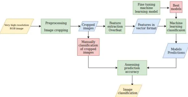
The general approach for the project is described in this section. The main goal was to detect if an image had palm trees, using a pre-trained convolutional neural network called OverFeat. This CNN architecture is not particularly trained to classify palm tree, nonetheless it excels at extracting features from images, meaning that it can describe in a mathematical context the geometries (objects) in an image. Cropping our data was part of the pre process, this was done to comply with data requirements from OverFeat, subsequently they were fed to the CNN for feature extraction and then classified using machine learning models. After assessing the accuracy, the best model was picked and used for visualization of results. A simplified methodological
flowchart is present in FigureFigure 3.3, yellow shapes represent the input data and
the final product, blue are intermediate results, green represent process and red input data for the process.
Figure 3.3: Flowchart depicting the methodology, yellow shapes represent beginning and finish product, blue intermediate results, green process, red input data
3.5.1 Tools
In this section the tools used are listed and briefly described, all the codes used are in Annex II
• ImageMagick version 6.9 was used for cropping the images. • OverFeat was used as a feature extractor.
• Python 3.6.5, numpy to load and manipulate the data set, scikit-learn was used for building and fine tuning the machine learning models, as well as making the predictions and matplotlib for plotting results.
• LibreOffice Calc was used for labeling the images, as well for assessing the accu-racy of the models
• QGIS 3.0 was used for creating the map of the study area, and for visualization of the results.
• SQLite for managing all the files and tables created
• All processes were done using a laptop with an Intel i7-6700HQ CPU @ 2.60GHz and 8 GB of DDR 3 RAM
3.6 Data Preprocessing
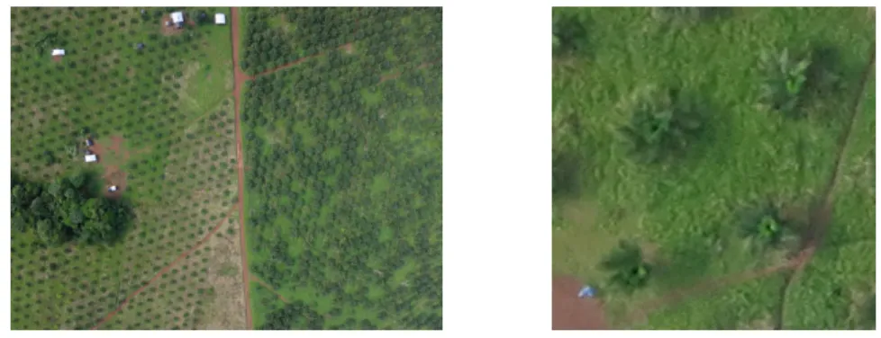
The purpose of this step is to generate images that can be analyzed with OverFeat. The original images have a size 4000 x 3000, each image was cropped into 192 tiles of 250 x 250, generating a total of 2112 images, the size was selected based on the
requirements of OverFeat. InFigure 3.4shows an example of image 2392 previously
to being pre processed (left) and an example of a tile from the cropped image (right). ImageMagick software was used for the cropping process, this is a free open source
software for displaying and manipulating images. To automate this process a bash1
script was created. It works by accessing the directory were the images are located it crops each image into 192 tiles, giving each tile an specific name and exports the results into a new directory, it repeats this process for each image. The output was classified depending on the presence of palms. The classification was performed via visual inspection and relying on the experience and knowledge of the area obtained during the aerial survey, nomenclature used is as followed, images containing palms were labeled as "1", otherwise a "0" was assigned.
Figure 3.4: Example of original image and cropped image
3 . 7 . O V E R F E A T A N D F E AT U R E E X T R AC T I O N
3.7
OverFeat
and Feature Extraction
OverFeatsoftware with its pre trained parameters was obtained from the creators
Github page, this software was made publicly available and provides a convolu-tional neural network based image classifier and feature extractor, in this study only the feature extractor was used. Again a bash script was used to automate the
pro-cess, the script takes as input cropped images produced onsection 3.6and feeds to
OverFeat, feature extractor. The output is a file that contains the mathematical
description of each shape found in each image (seeAnnex I), the description has a
magnitude and direction associated, therefore it can be considered a vector, that’s to say each feature extracted is represented as a vector.
These vectors were linked to the file containing labels for each image, producing a file that has image identification name, labels and a mathematical vector describing objects in the image, this file was used to train the machine learning models It’s ex-pected that the features extracted from images labeled as 0 and 1 vary substantially, making it possible to train a machine learning model to predict the label of the features extracted. this file was used to classify the vectors with machine learning models.
3.8 Machine Learning Models
Models were built using the python Scikit-learn library, a very common and wide spread tool in machine learning applications and scientific field. Many factors make it popular such as allowing the user to developed well known machine learning algo-rithms with a easy to use interface, it has a Berkley Software Distribution (BSD) license which impose minimal restrictions to its use and distribution, minimum requirements for ruing, ample documentation and examples, designed to maximize computational
efficiency and ease of use Pedregosa et al.2011.
Taking advantage of the capabilities and features of this library, several models were built they were:
• Support Vector Machine Linear • K Nearest Neighbor
• Decision Tree • Random Forest • Gradient Boost • Logistic Regression
The models are python scripts that use as input the file containing labels and
and 30% testing. The training data set was used for fine tuning the models, best parameters were selected and used to build the final model. The final product was a machine learning model that took as input a file containing vectors with no labels and produced a classification result for each vector. Finally to summarize the results a file was created with the classification provided by each model and the labels manually
given. Example scripts for the models and fine tuning process are inAnnex II
3.9 Visualization
To aid with the visualization of results a shape file for each image was created, the file contained name of each tile and classification result from each model as well as the manually given label, this allowed to compare between the classification result of each model.
3.10 Accuracy assessment
The predictions made by the models were compared with the labels given manually, for estimating the model accuracy. Overall accuracy was estimated using the formula:
OA= T P+ T N
T P+ T N + FP + FN
Where True Positive (TP), represent the positive cases correctly classified, True Negative (TN) the negative cases correctly classified, False Positive (FP), the negative cases classified as positives and False Negative (FN), the positive cases classified as negative.
C
h
a
p
t
e
r
4
R e s u lt s
4.1 Result overview
Results are presented in this chapter, very high resolution images were used as input for extracting features using a pre trained CNN, the features were used to train ma-chine learning models and to classify the images, the best model (SVM) achieved a accuracy of 97%.
4.2 Image preprocessing
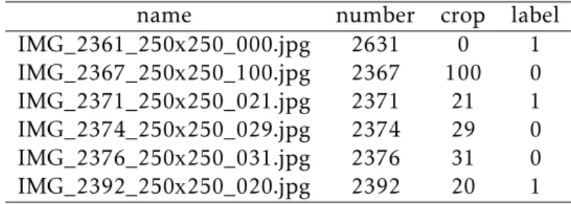
The cropping process for each image produced 192 tiles, generating a total of 2112 tiles. Each tile was given a name based on the number of the image and the number of tile. The list with names was used for labeling each tile depending on the presence or absence of palms, in total tiles labeled as "1" were 1001, meaning tiles with palms. The
remaining 1111 were labeled as "0" meaning no palms.Table 4.1provides an example
of the name given to a tile, the image it belongs to, the number of the tile under "crop" column and the label given. This table contains six records as an example of the results from the cropping process and the nomenclature used for each tile.
name number crop label
IMG_2361_250x250_000.jpg 2631 0 1 IMG_2367_250x250_100.jpg 2367 100 0 IMG_2371_250x250_021.jpg 2371 21 1 IMG_2374_250x250_029.jpg 2374 29 0 IMG_2376_250x250_031.jpg 2376 31 0 IMG_2392_250x250_020.jpg 2392 20 1
A detailed look of the objects present in the tiles is presented in Figure 4.1, it shows examples of the most representative objects of the study area, such as palm in development stages and mature, dirt road, forest, human made infrastructure and grassland. Items (a), (b) and (c) are tiles classified as 1, on the other hand items (d), (e) and (f) are classified as 0.
(a) (b) (c)
(d) (e) (f)
Figure 4.1: Examples of objects in the tiles
(a) Mature Palms (b) Palms in development stages (c) Dirt road (d) Infrastructure (e) Grassland (f) Forest
4.3 Feature extraction with OverFeat
The cropped images were processed with OverFeat, the output of this process was a file containing features from each tile. This is a vector of 4096 dimensions also called
CNN codes Karpathy (2016), specifically its a text file containing a list of values that
represent in a mathematical form the geometries found in the tiles. This data was
merged with the file generated insection 4.2and made it possible to relate labels to
the extracted features file. Examples of the extracted features for tiles labeled as "1" and "0" can be found inAnnex I.
4 . 4 . M AC H I N E L E A R N I N G M O D E L S C L A S S I F I CAT I O N R E S U LT S
4.4 Machine learning models classification results
The data set generate insection 4.3was used as input for training machine learning
models, the data was randomly split 70% for training and 30% testing, the models were
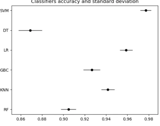
fine tuned and the best parameters were selected and then tested.Figure 4.2
summa-rizes the overall accuracy for each model, DT model achieved the lowest accuracy with 86.88 % ± 1.11 %, the second lowest was RF model with 90.50 % ± 0.71 %, the next three models had similar performance, GBC 92.66 % ± 0.79 %, KNN 94.18 % ± 0.63 % and LR 95.88 %±0.60 %, finally the SVM model had the highest accuracy with 97.73 %±0.51 %.
Figure 4.2: Overall accuracy and standard deviation of models
Table 4.2provides a similar description of the performance from the classifiers, but also includes values of sensitivity, specificity and precision. With regards to sensitivity the top three values follows the same order as observed in the overall accuracy, the forth highest value correspond to the RF model followed by GBC, this is the inverse order compared to overall accuracy. The lowest value corresponds to DT model, as is the case with overall accuracy. Values for specificity follow the same pattern as the overall accuracy, while the precision mirrors the order found in the sensitivity. Generally there’s a tendency that the DT model provides the lowest values regardless if is sensitivity, specificity, precision and therefore overall accuracy, random forest
performance better than DT, but not as good as the cluster form by GBC, KNN and LR, these three models have a similar performance but from the three GBC performs worst and LR achieving the best performance. Finally the SVM has the general highest performance from all the models.
Classifier Sensitivity Specificity Precision OA STD
SVM 97.30 98.11 97.89 97.73 0.51% LR 96.30 95.50 96.88 95.88 0.60% KNN 95.80 92.71 96.38 94.18 0.63% GBC 93.31 92.08 93.87 92.66 0.79% RF 94.71 86.68 95.28 90.48 0.71% DT 85.61 88.03 86.13 86.88 1.11%
Table 4.2: Accuracy assessment of Classification models
Performance of the models are presented in a more tangible matter inTable 4.3,
Table 4.4andTable 4.5. These confusion matrices represent the classification results of DT, GBC and SVM models, these three were compared because they represent the range of performances, the models presents the lowest and highest accuracy (DT, SVM) as well a model which performed in the middle ground between the to extremes (GBC). The tables have two rows and two columns, the header of the columns are "0" and "1" each representing the labels. The combination of rows and columns produce the values for true positives (TP) "1 1", tiles with palms correctly classified, true negatives (TN) "0 0", tiles with no palms correctly classified, false positives (FP)"0 1", tiles with no palms classified as having palms and "1 0" false negatives (FN), tiles with palms, that were not recognized by the model.
Reference
DT 0 1 Total Result
Predicted 0 978 144 1122
1 133 857 990
Total Result 1111 1001 2112
Table 4.3: Confusion matrix DT
Table 4.3presents the results for DT, the model with the lowest performance. Tiles classified as true positives amount 857 and true negatives 978, leaving a total of false positives of 144 and false negatives of 133.
Reference
GBC 0 1 Total Result
Predicted 0 1023 67 1090
1 88 934 1022
Total Result 1111 1001 2112
4 . 4 . M AC H I N E L E A R N I N G M O D E L S C L A S S I F I CAT I O N R E S U LT S
Table 4.4details the results of from gradient boost classifier, it represents the mid-dle ground of performance, it correctly classified 934 tiles with palms (true positives) and 1023 without palms (true negatives). False positives tiles sum a total of 67 and false negatives 88. Reference SVM 0 1 Total Result Predicted 0 1090 27 1117 1 21 974 995 Total Result 1111 1001 2112
Table 4.5: Confusion matrix SVM
Table 4.5 is focus on SVM, it classified correctly 974 from 1001 (True Positives) tiles with palm trees, in the case of tiles with no palm it classified correctly 1090 from 1111 (True Negatives). It classified 21 tiles as false negatives and 27 as false positives. The results presented in this section points to the SVM as being the best model, considering this tendency the image classification results will focus on the output provided by the SVM model.
4.4.1 SVM classification results
The SVM model used a linear kernel and the cost parameter was set to "C=1000". The linear kernel is recommend for data sets that can be linearly separated, also is less complex compared to the radial base kernel, thus it has less parameters that need fine
tuning. The cost parameter was obtained during the fine tuning process. InTable 4.6a
breakdown of the classification results per image, for example images 2376 and 2377
have no false negatives, this is in accordance to the description given insection 3.4, as
both this images contain a low percentage of palms, 22% and 1% respectively. Images 2371 and 2378 each have one tile classified as false negative.
The image with the most FN tiles is 2395 with 6 followed by 2389 with 5 and 2367 with 4, in these images palm represents at least 60% of the image, mixed with other features and land cover types such as forest and grasslands, dirt roads
The case with more FP tiles correspond to image 2371 with 5 cases, this image is composed by mature palm plantation, grassland and forest. Images 2376 and 2389 have 4 cases each of FP, this images are contrasting, as the first one is mainly natural forest and palm only represents 22% of the image and the lather is mainly palm tree plantation mix with forest, grassland and infrastructure. Is important to notice that image 2389 presents the most tiles wrongly classified with a total of 11, on the contrary image 2377 has no wrongly classified tiles. These two images are very different from
each other, the description provided insection 3.4shows that 2389 contains, several
land cover types, while image 2377 is mainly one land cover type corresponding to natural forest.
image Name TP TN FP FN 2361 171 19 0 2 2367 85 102 1 4 2371 109 77 5 1 2374 43 145 1 3 2376 9 179 4 0 2377 7 185 0 0 2378 27 162 2 1 2389 118 65 4 5 2392 170 19 0 3 2395 172 13 1 6 2402 63 124 3 2 Total 974 1090 21 27
Table 4.6: Classification results from SVM model for each image
Adding to the performance analysis,Figure 4.3shows the receiver operating
char-acteristics (ROC) curve. This analysis provides an insight into how well the model separates data into tiles containing palm and no palm. The horizontal axis contains the values of the false positive rate and in the vertical axis the true positive rate, this values are closely linked to the specificity and sensitivity respectively. The curve has an upward trend and levels out, near the top of graph, where the values of true positive rate is close to 1. The curve produces a high value for the metric area under the curve, in this case 95 % of the area of the graph is under the curve, this means that the model is good a separating the classes. As a reference the red dotted line that transverse the graph represents a 50% probability of correctly classifying the data or random chance. The further away the blue curve is from the red dotted line means that the model is better classifier compared to random chance.
4.5 Image Classification
Following the results from section 4.4, classification of the images was done based
on the SVM model. Predictions were made on the data extracted insection 4.3, and
compared to the labels manually given. A shape file with the classification results was created and used to aid visualization. This was done by stacking the shape file over the image file and categorizing the tiles by color. FP and FN tiles were given magenta and cyan respectively and a wider border to make then stand out. TP and TN negatives were given blue and red colors, less focused was given to this tiles as they were correctly classified.
An example of the classification is presented inFigure 4.4, emphasis is given to this
sub set of images as the contain most of miss classified tiles. The complete results for
all the images are presented inAnnex I. Item (a) is the classification results for image
4 . 5 . I M AG E C L A S S I F I CAT I O N
Figure 4.3: SVM classifier ROC curve
(b) corresponds to image 2371 which is a mix between palms and grasslands,it has the most cases of FN tiles from this sub set with 5 and only 1 case of FP. Image 2374 is showed in item (c) is similar in content to item (a) it presents 3 cases of FP and 1 of FN, item (d) is image 2378 is manly natural forest and a small patch of palms it has 2 cases of FN and 1 FP. Image 2389 corresponds to item (e) it has the most cases of miss classification, 4 FN and 5 FP, the image has a patch of natural forest palms, dirt roads and human made infrastructure. Item (f) is mainly palm trees and a bit of natural forest, it represents image 2395 and has 1 case of FN but the most FP cases from this sub set with 6. Item (g) is image 2402, it has a similar structure to item (a) and has 3 FN and 2 FP. In general features presented in this figure share the characteristics of of having several land cover types, meaning that the images contain transitions areas, where is not clearly
Figure 4.5presents examples of FP tiles, they were given label "0" but the model gave it a incorrect label of "1". In general this tiles can be found in transitions re-gions, for example item (a) is the transition zone between a patch of forest and palm plantation. Items (b) and (d) are grasslands but that have bush like plants that share resemblance with palm in developing stages, item (c) is forest land cover with several types of trees, it presents a complex structure that confused the classifier.
To have a closer look and analyze tiles classified as FN Figure 4.6 was created.
Examples in the figure show palms that were not recognized by the model, item (a) contains mature palms and a dirt road intersection, item (b) is showing some scatter palms not yet fully develop, item (c) are palms near the beginning of a patch of forest and item (e) are several mature palms and one small palm. In general this tiles show
(a) (b)
(c) (d)
(e) (f)
(g) (h)
(a) image 2367 (b) image 2371 (c) image 2374 (d) image 2378 (e) image 2389 (f)
image 2395(g) image 2402 (h) Legend
4 . 5 . I M AG E C L A S S I F I CAT I O N
(a) (b)
(c) (d)
Figure 4.5: Examples of tiles classified as False Positives (a) image 2389 (b) image 2371 (c) image 2374 (d) image 2389
palms mixed with other objects, close to transition zones, grainy images or with motion blur and palms with different development stages in the same tile.
The results presented inFigure 4.5andFigure 4.6paint a general picture of where
the model has problems with classification. In general terms this are areas with a lot
of different objects such as palms with dirt roads or forest. Figure 4.5is a close up
to examples of images classified as false positives. The figure present some common characteristics as they are low quality images, where detecting palms can be difficult even for humans, also some palms are in developing stages and as such don’t have the characteristic mature palm shape, other examples include isolated palms and transitions zones where the land cover changes from plantation to something different. A brief description of the tiles is presented next: (a), image 2389, there’s a small bush that resembles a palm, (b) image 2371, grassland with and bushes, (c) image 2374, several trees forming a complex structure and (d) image 2389, the image is blurry and
share some of the same characteristics, errors where located near transitions zones, near the boundaries of the plantation or tiles with different land covers. It was also noted that tiles where there is a mix of palms in different development stages are problematic, palms in developing stage have a tone of color that makes then similar to bushes, thus making them difficult to detect even to the human eye. The tiles presented in the figure belong to (a) image 2392, it has mature palms and a dirt road, (b) image 2389, small palms and grassland,(c) image 2374, small palms next to forest and (d) image 2395, mature palms mixed with small palms.
(a) (b)
(c) (d)
Figure 4.6: Examples of tiles classified as False Negatives (a) image 2392 (b) image 2389 (c) image 2374 (d) image 2395
C
h
a
p
t
e
r
5
D i s c u s s i o n a n d C o n c l u s i o n
A discussion of the results is presented in this chapter, in section 5.1 an in depth
discussion of each result is presented follow by the main limitations of the study and
future works,section 5.2presents the conclusion of this work
5.1 Discussion
CNN have proven to excel at image classification tasks in a remote sensing context,
some cases studies and examples were disscussed in 2.4. Most of this applications
focus on the analysis of satellite images, as this type of data sets are more accessible in comparison to very high resolution UAV imagery. This translates into less research done with very high resolution images and CNN. The method propose in this study tries to narrow this gap by classifying palm tree images obtained from an aerial survey, with the aid of CNN and machine learning algorithms.
The methods was tested by using the pre trained feature extractor OverFeat, the output of this network was used for training machine learning models to performance classifying tasks, the results prove that the features extracted are suitable for
classify-ing very high resolution images. In the studies by Nogueira et al. (2017) and Penatti
et al. (2015) concluded that a trained CNN to recognize everyday objects, can
gener-alize features well enough to be used in a remote sensing context, this aligns with the findings of this study.
The data used for this method consisted of 11 images, these were selected based on their quality and being representative of the study area. The images required a size of 256 x 256 to analyze them with OverFeat, this lead to cropping each image and producing a total of 2112 tiles. Small data sets like this are not enough to train from scratch a CNN. In this cases the recommend approach is to use transfer learning
Nogueira et al. (2017) and Sharif Razavian et al. (2014).
As seen in Figure 4.1, Figure 4.5andFigure 4.6the cropping process, generates
tiles that in most cases contain more than one single palm tree or cases that only partially show palms. Finding a cropping size that complied with the requirements of
OverFeatand synced perfectly with the spatial distribution of the plantation, so that
only one palm was present per tile was not practical. Therefore this method cannot localized or detect the palms in the tile, rather it can be used as a classification method, by labeling if the tile contains palm or not.
In general it can be said that OverFeat was able to recognize the difference be-tween tiles with palms and no palms, proof of this is the classification results from the several machine learning models (Table 4.2), this was possible due to the difference be-tween the features that describe the two classes, as their characteristics were different enough for the ML models to recognize. From the results presented by Nogueira et al.
(2017), Zhang et al. (2015), and Zhou et al. (2016), it was expected for the CNN to
provide features, that would effectivily separate objects in the images. Is important to note that this results were based on satellite imagery, while the results obtained from this study were based on very high resolution UAV imagery. Considering this, it can be said that a pre trained CNN can effectively be used in image recognition task, in the particular case of very high resolution aerial images
In regards to the machine learning models, performance observed coincides with previous studies, in the case of DT, this method is susceptible to data set size, Pal and
Mather (2003) showed that accuracy has a positive correlation with training size, this
notion was also confirmed by Rogan et al. (2008), this study found that decreasing
the training samples implies a reduction in accuracy. On the other hand findings by
Foody and Mathur (2004) determined that SVM is less sensible to small sample sized
compared to DT. This trend can also be observed in the results (section 4.4), where DT has the lowest accuracy and SVM the highest, it can inferred that the data set was not big enough for the DT model to have an optimal performance and accuracy, but regardless of the size the SVM still performed well. This helps to explain the reason SVM is one of the most popular ML methods for image classification task, Bazi and Melgani (2018), Petropoulos et al. (2012), Salberg (2015), and Waske et al. (2009).
In the study by Lawrence and Moran (2015), they systematically tested several
machine learning methods, with 30 different data sets and found that ensemble meth-ods like random forest performed overall better, nonetheless in some of the data sets SVM performed better. With this findings they concluded the best algorithm for image classification task is dependent of the data set. In this study two ensemble methods were tested, random forest and gradient boost classifier, the first in general performed poorly in comparison to the rest, while the performance of the lather was consider a middle point between all the models. The systematical testing done by Lawrence and
Moran (2015), found that assemble methods outperform the rest, in contrast our study