1 A Work Project, presented as part of the requirements for the Award of a Research Master
Degree in Economics from the NOVA – School of Business and Economics
Optimality of bailout lending when asymmetric information increases sovereign yields
Maria Leonor Pizarro Beleza Cortez Queiró, 13
A Project carried out on the Research Master in Economics Program, under the supervision of:
Professor Guido Maretto January 2016
2 Optimality of bailout lending when asymmetric information increases sovereign yields
Abstract
Is the sovereign debt market information-sensitive to the true borrowing amount? If yes, does asymmetric information affect welfare? What mechanism can improve the welfare of transparent governments? To address these questions, this paper builds a sovereign debt model in which the government can be transparent or opaque. The model predicts that asymmetric information about the government’s type decreases the welfare of a transparent government, by either inducing a transfer of welfare to an opaque government through the market price or by leading to market breakdown. Building on this model, I develop a mechanism of inspection and penalties on cheating governments and conclude that bailout lending when market yields rise as a result of this information friction does not necessarily improve the welfare of transparent governments compared to market lending, if the market still provides lending.
3 Contents
1. Introduction
2. Relation with the literature
3. Chapter I: Information-sensitivity of the market to the true borrowing amount 3.1. The baseline model
3.1.1. Fundamentals
3.1.2. Information structure
3.1.3. Motivation to borrow and gains from trade 3.1.4. Timing
3.2. Equilibrium
3.2.1. Equilibrium under symmetric information and a type 1 3.2.2. Equilibrium under symmetric information and a type 2 3.2.3. Equilibrium under asymmetric information about type 3.3. Welfare
4. Chapter II: A mechanism of costly inspection and penalties for cheating 4.1. The model with the mechanism
4.2. Equilibrium under commitment to inspect the government 4.3. Equilibrium under no commitment to inspect the government
5. Chapter III: Who and when benefits from the introduction of a mechanism? 5.1. When does the welfare of a type 1 improve?
5.2. When does the welfare of a type 2 improve? 5.3. Does aggregate welfare improve?
4 Tables
1. Market equilibrium under symmetric information and type 1 2. Market equilibrium under symmetric information and type 2 3. Market equilibrium under asymmetric information about type 4. Market equilibrium 1 under commitment mechanism
5. Market equilibrium 2 under commitment mechanism
5 Figures
1. Greece’s sovereign yields (%) 2. Portugal’s sovereign yields (%)
3. Parameter space of existence of commitment mechanism equilibrium 1 4. Parameter space of existence of commitment mechanism equilibrium 2
5. Parameter space of existence of no commitment mechanism equilibria 1 and 3 6. Inspection mechanism that implements lending for the highest c
7. Parameter space where “no mechanism” implements lending for higher c values than commitment mechanism Equilibrium 1
6
1. Introduction
In October 2009, the newly elected government in Greece announced a revision of the estimate for its 2009 deficit from 6% - 8% to 12,5%, saying that estimates provided by the previous government had been significantly understated1. It also revised Greece’s 2008 deficit from 5% to 7,7%2. Greek sovereign yields immediately soared.
In January 2010, a report published by the European Commission3 said that Greece’s figures were “so unreliable that its budget deficit and public debt could be higher than the numbers claimed by the Greek government in October”. According to the news4, the report said that “a substantial number of unanswered questions and pending issues still remain in some key areas (…) and it cannot be excluded that this will lead to further revisions of Greek government deficit and debt data, particularly for 2008 but possibly also for previous years”. In April 2010, the estimate was again revised upwards and the final estimate is 15,2%5. In May 2010, Greece requested an official bailout from the IMF and the EU6.
Although the Commission said that EU fiscal data were generally of high quality and that Greece was an isolated case, it also said that the EU lacked audit powers and so “relied heavily on the goodwill and integrity of member-states to supply accurate data”. Facts are that in January 2010 sovereign yields in Portugal also sky-rocketed, without any policy announcement at the national or European level about Portugal, and in May 2011 Portugal requested an official bailout from the IMF and the EU7.
1 Financial Times, October 20, 2009 “Greece vows action to cut budget deficit” 2 Financial Times, January 12, 2010 “Greece condemned for falsifying data”
3 Brussels, 8.1.2010 COM(2010) 1 final “Report on Greek Government deficit and debt statistics” 4 Financial Times, January 12, 2010 “Greece condemned for falsifying data”
5 Source: Eurostat
6 IMF Press Release No. 10/176, May 2, 2010 7 IMF Press Release No. 11/190, May 20, 2011
7 Figure 1: Greece’s sovereign yields (%)8
Figure 2: Portugal’s sovereign yields (%)9
8 Source: Bloomberg 9 Source: Bloomberg 0 5 10 15 20 25 0 1 -0 1 -2 0 0 7 0 1 -0 4 -2 0 0 7 0 1 -0 7 -2 0 0 7 0 1 -1 0 -2 0 0 7 0 1 -0 1 -2 0 0 8 0 1 -0 4 -2 0 0 8 0 1 -0 7 -2 0 0 8 0 1 -1 0 -2 0 0 8 0 1 -0 1 -2 0 0 9 0 1 -0 4 -2 0 0 9 0 1 -0 7 -2 0 0 9 0 1 -1 0 -2 0 0 9 0 1 -0 1 -2 0 1 0 0 1 -0 4 -2 0 1 0 0 1 -0 7 -2 0 1 0 0 1 -1 0 -2 0 1 0 0 1 -0 1 -2 0 1 1 0 1 -0 4 -2 0 1 1 0 1 -0 7 -2 0 1 1 0 1 -1 0 -2 0 1 1 0 1 -0 1 -2 0 1 2 0 1 -0 4 -2 0 1 2 0 1 -0 7 -2 0 1 2 0 1 -1 0 -2 0 1 2 0 1 -0 1 -2 0 1 3 0 1 -0 4 -2 0 1 3 0 1 -0 7 -2 0 1 3 0 1 -1 0 -2 0 1 3 0 1 -0 1 -2 0 1 4 0 1 -0 4 -2 0 1 4 0 1 -0 7 -2 0 1 4 0 1 -1 0 -2 0 1 4 0 1 -0 1 -2 0 1 5 0 1 -0 4 -2 0 1 5 0 1 -0 7 -2 0 1 5 0 1 -1 0 -2 0 1 5 0 1 -0 1 -2 0 1 6
GgGb2yr Index GgGb5 Index GgGb10 Index
0 5 10 15 20 25 0 1 -0 1 -2 0 0 7 0 1 -0 4 -2 0 0 7 0 1 -0 7 -2 0 0 7 0 1 -1 0 -2 0 0 7 0 1 -0 1 -2 0 0 8 0 1 -0 4 -2 0 0 8 0 1 -0 7 -2 0 0 8 0 1 -1 0 -2 0 0 8 0 1 -0 1 -2 0 0 9 0 1 -0 4 -2 0 0 9 0 1 -0 7 -2 0 0 9 0 1 -1 0 -2 0 0 9 0 1 -0 1 -2 0 1 0 0 1 -0 4 -2 0 1 0 0 1 -0 7 -2 0 1 0 0 1 -1 0 -2 0 1 0 0 1 -0 1 -2 0 1 1 0 1 -0 4 -2 0 1 1 0 1 -0 7 -2 0 1 1 0 1 -1 0 -2 0 1 1 0 1 -0 1 -2 0 1 2 0 1 -0 4 -2 0 1 2 0 1 -0 7 -2 0 1 2 0 1 -1 0 -2 0 1 2 0 1 -0 1 -2 0 1 3 0 1 -0 4 -2 0 1 3 0 1 -0 7 -2 0 1 3 0 1 -1 0 -2 0 1 3 0 1 -0 1 -2 0 1 4 0 1 -0 4 -2 0 1 4 0 1 -0 7 -2 0 1 4 0 1 -1 0 -2 0 1 4 0 1 -0 1 -2 0 1 5 0 1 -0 4 -2 0 1 5 0 1 -0 7 -2 0 1 5 0 1 -1 0 -2 0 1 5 0 1 -0 1 -2 0 1 6
8 The recent sovereign debt crisis in Europe revived the role that information might have on the sovereign debt market. Kletzer (1984) showed that lack of observability of the true amount of borrowing by a government leads to a loss of welfare, because lenders treat the government as a price taker rather than as a price maker. The loss of the first-mover advantage implies that the equilibrium of the market under lack of observability is weakly dominated by the equilibrium of the market under observability. Kletzer’s empirical motivation was the experience of the less-developed countries, during the late 1970s. The empirical motivation of this paper is the substantial rise of Portugal’s sovereign debt yields in 2010, shortly after Greece revealed that it had misreported its true borrowing levels. Although investors did not know whether Portugal also misreported its numbers or not, one interpretation is that the Greek revelation showed that it was possible to hide debt even within the EU.
This paper therefore aims at building a formal structure to study the effect of not knowing whether a government can hide debt or not. Building upon the model, the second aim of this paper is to investigate the effect of allowing for a mechanism of inspection with penalties for cheating, which can be interpreted as bailout lending or as the introduction of penalty clauses on bond contracts enforceable by a supranational authority, on the welfare of a well-behaved government. Given the lack of such a clear supranational authority in reality, this paper can be best seen as a model of bailout lending under asymmetric information.
The structure of this thesis is the following: chapter I studies the information-sensitivity of the market by building a sovereign debt model with one government type that is transparent and one type that is opaque, where type is private information to the government. It also studies the effect of asymmetric information on welfare. Chapter II develops a mechanism of costly inspection of the government’s true amount of borrowing and infliction of penalties on a government found cheating. Chapter III analyzes the extent to which the introduction of this
9 mechanism increases the welfare of each government type. The paper ends with a summary of the conclusions.
2. Relation with the literature
The central theme of the sovereign debt literature is the risk of repudiation. The breakthrough was made by Eaton and Gersovitz (1981), where a theory about sovereign default was first developed. The theory says that sovereign lending exists in equilibrium to the extent that a government sustains a reputation as a good debtor. It is the fear of being excluded from the market following a default that keeps sovereign debtors repaying. In that sense, the more a country values inter-temporal consumption smoothing, for example, the higher the amounts of debt that it will be served by the market, since investors know about the government’s incentives to repay. This is called the reputational approach to sovereign debt and has been followed by several authors throughout time (Kletzer (1984), Grossman and Van Huyck (1988), Cole and Kehoe (1998 and 2000), Wright (2002) and Arellano (2008), for example).
A parallel theory about sovereign default was developed by Bullow and Rogoff (1989), defending that lending to sovereigns is supported by the extent to which lenders have legal rights to impose sanctions on a defaulting government, such as impeding a country’s trade or seizing its financial assets abroad. This approach – the direct sanctions approach – differs substantially from the reputational one, since, precisely, the reputational approach lies on the assumption that sovereign lending does not, by the nature of a sovereign as an immune debtor, rely on collateral. Both approaches explain the existence of debt ceilings on governments debt (that is, threshold levels of debt above which lenders are not willing to lend, even though a sovereign might be willing to pay a higher interest rate) and both model the price schedule of loans as a decreasing price schedule on the amount borrowed (the higher the amount of the loan, the higher the relative incentive to repudiate on it, according to the reputational approach, and the lower the collateral per unit of debt, according to the direct sanctions approach). Both
10 these features induce a decrease on the welfare of the sovereign, when compared to perfectly enforceable debt.
Formally, time consistency is a fundamental requirement when formalizing a sovereign debt market equilibrium, as sovereign debtors decide to pay or to default at each period in time weighing the loss of repaying against the loss of defaulting, as opposed to following a previously defined repayment plan. Accordingly, the planning/Ramsey formulation should not be used to formalize the equilibrium, since the latter does not require time consistency, when the agents can re-optimize within periods (that is, subgame-perfection in a sequential game). As a result of imperfect enforcement and sequential decision-making, the literature explains limited risk-sharing in the sovereign debt market between risk-averse sovereign debtors and risk neutral lenders (for example, Grossman and Van Huyck (1988)). Sovereign debt is widely modeled as state-non contingent bonds, because state-contingent debt is not sustainable in equilibrium when the debtor can repudiate on the contingencies established in the contract when it benefits from doing so.
The introduction of the possibility to reschedule (or, more broadly, to renegotiate) sovereign debt enriched the descriptive power of sovereign debt models. Allowing for debt renegotiation impacts the debt ceilings imposed on sovereigns, since lenders can receive partial repayments (a model of partial default with a simple modeling of bargaining powers can be found in Sachs and Cohen (1982), while models of partial default with more developed bargaining processes can be found in Fernandez and Rosenthal (1990) and Bulow and Rogoff (1989)).
The problem of multiplicity of equilibria has been studied in this market. The ways in which multiplicity may arise are studied, for example, by Calvo (1988), Cole and Kehoe (2000) and Ayres, Navarro, Nicolini and Teles (2015).
11 Quantitative models have also been built with country-specific calibrations, allowing for positive explanations of empirically observed events in sovereign debt markets (for example, Aguiar and Gopinath (2006) and Arellano (2008)).
Although the sovereign debt market literature has developed continuously throughout time, the topic of information frictions remains relatively understudied. Kletzer (1984) was the first to bring about the role of the information structure in the sovereign debt market. Kletzer’s main insight is that lack of observability of the true amount of borrowing by a government leads to a loss of welfare, because lenders treat the government as a price taker rather than as a price maker. The loss of the first-mover advantage is abstracted from in the majority of sovereign debt models, since they implicitly assume that investors are able to know the amount of debt that they are pricing. The order in which players move that this introduces can be related to Ayres et al. (2015) and Lorenzoni and Werning (2013), since both those papers also change the usually implicit assumptions regarding the timing of the borrowing relationship. Lorenzoni and Werning explain it as a lack of commitment to previous borrowing announcements, since the borrowing needs of the government are only realized after lenders have fixed prices. In this model, I explain timing differences with asymmetric information. My model and those other two share in common the fact that all departure from the standard sovereign debt assumption of the first-mover timing, which leads to important qualitative changes in the results.
Atkeson (1991) studies asymmetric information regarding the use of borrowed funds. He assumes that lenders are unable to observe whether the government uses loans for consumption or investment and assumes that lenders cannot perfectly inspect the use of borrowed funds by the government, for which reason the latter has incentives to overuse the funds for consumption. There, loan repayment is more attractive for higher levels of output and output increases with investment. The moral hazard potential to overuse borrowed funds for consumption makes the optimal contract demand high repayments when the realization of income is so low that it
12 indicates less than optimal investment. This information asymmetry and its consequences on the optimal debt contract are meant to provide an explanation for why state contingent contracts provide only partial insurance to risk-averse governments in face of adverse output shocks. The asymmetric information price schedule of my model accounts for the risk of debt dilution. Debt dilution risk and the resulting haircut on the price decrease welfare, by inducing adverse selection and increasing the cost of debt. Therefore, the search for a remedy to overcome the problem of debt dilution proves important. The topic of debt dilution and the study of remedies to overcome that distortion have been present in the literature. One proposed solution is the introduction of seniority clauses (see for example Chatterjee and Eyigungor (2015)). However, remedies such as seniority clauses would not overcome the debt dilution problem if it arises due to asymmetries of information. The introduction of costly inspection is adequate to deal with unobserved action (see Townsend (1979)). Additionally, in my model, the mechanism designed does not suffer from the existence problem present in Rothschild and Stiglitz (1976), because the amount of the penalty is exogenous to the model.
3. Chapter I: information-sensitivity of the market
3.1 The baseline model
3.1.1 Fundamentals (time horizon, agents, endowments and payoffs)
There are two periods, denoted 𝑡 ∈ {0,1}. At 𝑡 = 0, the government receives an exogenous endowment of 𝑦0 = 0, and has a legacy debt 𝑐 > 0. At 𝑡 = 1, the government receives an exogenous endowment 𝑦1, which is randomly drawn from a uniform distribution, whose support is [𝑦0, 𝑦], where 𝑦 takes the value of 1. The government is risk neutral, does not
discount the future and maximizes the following linear lifetime payoff over consumption: 𝑐0+ 𝑐1
A set of small investors has funds which they can lend to the government, in the form of state-non contingent discount bonds 𝐵 at a price 𝑞 with one period maturity. Since lenders are small,
13 no individual lender can be a single lender to the government. Lenders are risk neutral, do not discount the future and are perfectly competitive. 𝜋 denotes the profit from investing in a sovereign bond. The expected profit at the time of the investment is:
𝐸(𝜋) = −𝑞𝐵 + 𝐵 ∗ 𝑟𝑒𝑝𝑎𝑦𝑚𝑒𝑛𝑡 𝑝𝑟𝑜𝑏𝑎𝑏𝑖𝑙𝑖𝑡𝑦 + 0 ∗ 𝑑𝑒𝑓𝑎𝑢𝑙𝑡 𝑝𝑟𝑜𝑏𝑎𝑏𝑖𝑙𝑖𝑡𝑦 In equilibrium, the bond price 𝑞 must satisfy:
𝐸(𝜋) = 0
The government can borrow 𝐵 from lenders at 𝑡 = 0. If 𝑞𝐵 < 𝑐, the government defaults at 𝑡 = 0, since 𝑐 > 𝑦0. If the government defaults at 𝑡 = 0, it does not move on to period 1. If it
repays, it moves on and receives 𝑦1 at 𝑡 = 1. At 𝑡 = 1, the government can either repay its loan and receive 𝑦1− 𝐵 or repudiate on its loan and receive 𝑦0, the lower bound of the distribution of 𝑦1 (this default cost follows Ayres et al. (2015)).
3.1.2 Information structure
There are two government types: type 1 can only borrow 𝐵 and type 2 can borrow 𝐵 and 𝐻, with 𝐻 taking values in [0, 𝐾]. Within this environment, I analyze two information structures: first, a structure of symmetric information, in which the government’s type is public information; second, a structure of asymmetric information, where the government’s type is private information to the government. A type 1 government can be seen as a transparent government, which cannot deviate from the borrowing announcement made to the public. A type 2 can be seen as a government who can end up borrowing more than the amount announced by the time lenders fix the bond price. In the model, I say that a type 2 can hide borrowing.
3.1.3 Motivation to borrow and gains from trade
𝑦0 < 𝑐, which implies that the government needs to borrow in order to avoid default at 𝑡 = 0. If the government defaults at 𝑡 = 0, its payoff is 0. If the government repays, it moves on to period 1 and its period 1 payoff is bounded below by 0, since the government can repudiate on its loan and the default cost is a payoff of 0. Hence, borrowing at 𝑡 = 0 weakly dominates
14 autarky. Lenders make zero expected profits in a lending equilibrium, so they have a payoff of 0 either by participating in the market or by not participating. So aggregate surplus is weakly higher in a lending equilibrium than in an autarky one. The gains from trade are the transfer of wealth that the government can make between periods through trading bonds.
3.1.4 Timing
Formally, the government’s type translates into a specific timing of the loan relationship, since private information regarding the government’s type introduces an information friction which is taken into account by lenders when pricing bonds. If the government is of type 1, it moves first by announcing 𝐵 and lenders move second, by offering 𝑞. If the government is of type 2, the government moves first by announcing 𝐵, then lenders offer 𝑞, but then the government moves again by choosing 𝐻. Both 𝐵 and 𝐻 affect the repayment probability of 𝐵, so lenders take into account what they anticipate the choice of 𝐻 to be when choosing 𝑞. In that sense, the government behaves as a price-taker in 𝐻. The timing of the game is the following: at 𝑡 = 0, both types announce 𝐵. Then investors decide 𝑞 through take-it-or-leave-it offers. Then, a type 2 has another move, which is the choice of 𝐻. At 𝑡 = 1, income 𝑦1 is exogenously realized and
a type 1 choses to repay or default on 𝐵 and a type 2 choses to repay or default on 𝐵 + 𝐻. After a default, both types enjoy the autarky payoff while repayment yields 𝑦1 net of paid funds. This
is summarized in the timeline below:
3.2 Equilibrium
3.2.1 Equilibrium under symmetric information and a type 1 government
When lenders know they face a type 1 government, the timing of the model becomes the following: Government announces B Investors offer discount price Type 2 Government chooses H Period 1 income is realized Government repays or defaults Government enjoys income
15 A. Decision problem of the government
At 𝑡 = 1, the payoff from defaulting is:
𝑦0 The payoff from repaying is:
𝑦1− 𝐵
The payoff-maximizing government therefore repays at 𝑡 = 1 if and only if: 𝑦1 > 𝑦0+ 𝐵
At 𝑡 = 0, the government chooses the amount of debt to borrow (𝐵) in such a way as to maximize its lifetime payoff, knowing that it will optimally choose to repay or default at 𝑡 = 1. So the government chooses 𝐵 to solve the following problem:
max 𝐵 𝑦0− 𝑐 + 𝑞𝐵 + ∫ (0)𝑑𝐹(𝑦1) + ∫ (𝑦1− 𝐵)𝑑𝐹(𝑦1) 1 𝐵 𝐵 0
The initial part of the objective function is the government’s payoff at 𝑡 = 0, which is its endowment net of bills plus the proceeds from borrowing. The second part of the objective function is the government’s expected payoff at 𝑡 = 1, which is either its endowment net of debt repayment or the autarky income, taking into account the optimal repayment choice. The repayment decision is probabilistic at 𝑡 = 0, since the distribution of 𝑦1 is public information. The decision to repay follows the spirit of the sovereign debt literature in that it is a strategic decision: a government repudiates on its debt unless its payoff is higher if it repays. However, this is not apparent in this model, since the default cost is modeled to be the lower bound of the distribution of period 1’s income. Hence, the choice to repay or default becomes mechanical and determined by ability-to-pay, since the default cost is as strong as an income of 0.
Government announces B Investors offer discount price Period 1 income is realized Government repays or defaults Government enjoys income
16 B. Equilibrium bond price
Since each creditor is small, under perfect competition the requirement for zero expected profits implies that they all offer the same price. Since the risk-free rate in this model is 0, the expected return of lending in this economy must be 0.
𝐸(𝜋) = 0
Since bonds are discount bonds, the equilibrium bond price is pinned down by the relationship: 𝑞 = 1 − 𝐵
The bond price is the repayment probability of the loan, since, for each unit lent, lenders receive one unit in case of repayment and zero in case of default. This bond price schedule is the supply of loan contracts, since it defines a set of pairs of loan amounts and prices that achieve zero expected profits, given optimal default behavior by the government.
Moreover, lenders will not lend amounts of debt for which the probability of repayment is 0, so, in equilibrium, it must be the case that:
𝐵 ≤ 1
Imperfect enforcement is the reason behind a decreasing bond price schedule and credit ceilings on sovereigns. As the loan increases, so does default probability, which decreases the price.
C. Equilibrium lending
Equilibrium is defined as: prices clear markets given available information and quantities are optimal. An equilibrium is then a pair (𝑞, 𝐵) which solves:
max 𝐵 −𝑐 + 𝑞𝐵 + ∫ 0𝑑𝐹(𝑦1) + ∫ (𝑦1− 𝐵)𝑑𝐹(𝑦1) 1 𝐵 𝐵 0 𝑠. 𝑡. 𝑞 = 1 − 𝐵 𝑞𝐵 ≥ 𝑐 𝐵 ≤ 1
17 The first constraint is the zero profit condition. The second constraint is the government’s budget constraint. The third constraint is the debt ceiling. The equilibrium borrowing amount can be shown to be:
𝐵 =1 2−
1
2√1 − 4𝑐
This equilibrium amount is the minimum amount necessary to pay back bills 𝑐 and avoid default at 𝑡 = 0. The intuition is the following: a decreasing loan price schedule implies that the marginal benefit of debt is lower than its marginal cost, for any debt size.
𝑚𝑎𝑟𝑔𝑖𝑛𝑎𝑙 𝑏𝑒𝑛𝑒𝑓𝑖𝑡 𝑜𝑓 𝐵 = 1 − 2𝐵 𝑚𝑎𝑟𝑖𝑔𝑛𝑎𝑙 𝑐𝑜𝑠𝑡 𝑜𝑓 𝐵 = 1 − 𝐵
While the marginal benefit of debt is its repayment probability, since that is what lenders receive per unit of debt in expected terms, the marginal cost of debt is the repayment probability of the loan in case of repayment and the default cost in case of default. Since the default cost is not zero (the government loses its period 1’s income), the expected cost of the loan is higher than its repayment probability. This results from the fact that, although sovereigns can repudiate on their loans, they do suffer a cost for defaulting, which is not received by the creditors.
Since the government’s payoff is decreasing in 𝐵, there must be an upper bound on 𝑐 for which it is individually rational to borrow. Since the government’s payoff at 𝑡 = 1 is bounded below by 0, borrowing is individually rational insofar as 𝑐 can be raised at the prevailing price schedule. Therefore, borrowing is individually rational for 𝑐 < 𝑞𝐵. With 𝐵 optimally chosen, this yields the upper bound 𝑐 <14. These findings are summarized in Lemma 1.
Lemma 1: With symmetric information, lending exists in equilibrium for 𝑐 < 14 for a type 1
government.
Table 1 describes the market equilibrium as a function of c:
18 Information structure Symmetric (Type 1 Government)
c (funding needs) 𝑐 ≤1 4 𝑐 > 1 4 Equilibrium Borrowing 𝐵 =1 2− 1 2√1 − 4𝑐 0 Equilibrium price schedule 𝑞 =1 2+ 1 2√1 − 4𝑐 𝑞 = 0 Expected payoff Government 1 4+ 1 4√1 − 4𝑐 − 𝑐 2 0
Lenders’ expected profit 0 0
Default probability 1
2− 1
2√1 − 4𝑐 0
3.2.2 Equilibrium under symmetric information and a type 2 government When lenders know they face a type 2 government, the timing becomes:
A. Decision problem of the government
The problem is solved by backward induction, as in the case of a type 1 government, except that there is one additional layer of decision making, which is the government’s choice of 𝐻. At 𝑡 = 1, the payoff from defaulting is:
𝑦0
The payoff from not defaulting is:
𝑦1− 𝐵 − 𝐻
Therefore, a payoff maximizing government repays at 𝑡 = 1 if and only if:
Government announces B Investors offer discount price Government chooses H Period 1 income is realized Government repays or defaults Government enjoys income
19 𝑦1 > 𝑦0+ 𝐵 + 𝐻
At 𝑡 = 0, after a type 2 has announced 𝐵 and lenders have offered 𝑞, a type 2 chooses 𝐻 to maximize its payoff. The choice of 𝐻 therefore solves the following problem:
max 𝐻 𝑦0− 𝑐 + 𝑞 ∗ (𝐵 + 𝐻) + ∫ 0𝑑𝐹(𝑦1) + ∫ (𝑦1− (𝐵 + 𝐻))𝑑𝐹(𝑦1) 1 𝐵+𝐻 𝐵+𝐻 0
The solution is that the hiding choice of a type 2 government is a corner solution: either 0 or K. Since lenders do not observe H, the price of B is not a function of H. In order for it to be incentive compatible for a type 2 to hide a positive amount of H, the price has to be sufficiently attractive. A sufficiently attractive price is a price that is sufficiently higher than the repayment probability of 𝐵 + 𝐻. Only in that case is the marginal benefit of loans higher than its marginal cost and it is optimal to choose a borrowing amount larger than the necessary to avoid default in period 0. Otherwise, the increase in consumption at 𝑡 = 0 attained through hiding is not enough to compensate for the cost in period 1 of that same hiding (an increase in repayment or a higher probability of default) and the government’s payoff actually decreases by choosing a positive amount of 𝐻. Formally, lenders choose to hide H if and only if:
max 𝐵 𝑦0− 𝑐 + 𝑞 ∗ (𝐵 + 𝐻) + ∫ 0𝑑𝐹(𝑦1) + ∫ (𝑦1− (𝐵 + 𝐻))𝑑𝐹(𝑦1) 1 𝐵+𝐻 𝐵+𝐻 0 > max 𝐵 𝑦0− 𝑐 + 𝑞 ∗ (𝐵) + ∫ 0𝑑𝐹(𝑦1) + ∫ (𝑦1− (𝐵))𝑑𝐹(𝑦1) 1 𝐵 𝐵 0
This yields a discontinuous demand function for 𝐻: either 0 or K. In my model, since the government is risk neutral and the productivity of loans is their discount price, which, once fixed, does not decrease with loans, if it is profitable to borrow one additional unit once the price is fixed, it is profitable to borrow all possible additional units. Although a higher default probability decreases the government’s future expected consumption, the inter-temporal allocation of consumption is not a concern under risk neutrality.
20 With perfect competition, the price schedule is pinned down by the relation:
𝐸(𝜋) = 0
Since lenders cannot observe 𝐻, the supply of loans schedule is of the form: 𝑞 = 1 − 𝐵 − 𝑥
Where 𝑥 is the conjectured level of hiding.
Fact 1: With symmetric information about the government’s type, investors only lend to a type
2 government on its demand curve.
A demand curve amounts to an incentive compatibility constraint. In this model, since the choice of H is either 0 or K and since if lenders price H = 0 the price is sufficiently high for a type 2 government to deviate to H = K, a necessary condition for a lending equilibrium is that lenders price the default risk of K. So the equilibrium bond price schedule is:
𝑞 = 1 − 𝐵 − 𝐾
Moreover, lenders will not lend amounts of debt for which the probability of repayment is 0, so in equilibrium it has to be the case that:
𝐵 + 𝐾 ≤ 1 C. Equilibrium lending
The equilibrium price schedule is such that there is no loan amount (including hidden borrowing) whose price can be higher than its repayment probability, so there is no opportunity for profitable hiding. Since hiding is unprofitable, the optimal choice of total debt is the minimum necessary to avoid default at 𝑡 = 0. So the equilibrium B solves:
𝑐 = (1 − 𝐵 − 𝐾) ∗ (𝐵 + 𝐾) Which is: 𝐵 =1 2− 1 2√1 − 4𝑐 − 𝐾 And the choice of 𝐻 is:
21 Since hiding is unprofitable, the government will borrow as least as possible. That is achieved by decreasing 𝐵 by 𝐾. It must be IR for a type 2 government to participate in the market. Since borrowing is IR as long as it can raise its funding needs in the market so as to avoid default at 𝑡 = 0, the binding constraint on 𝑐 is the price schedule. Since 𝐵 is decreased by 𝐾, the price schedule ends up being equal to that of a type 1, which yields the same upper bound on 𝑐.
Lemma 2: With symmetric information about the government’s type and about the value of 𝐾,
lending exists in equilibrium for 𝑐 <14 for a type 2 government.
Under asymmetric information about total borrowing, the market is only in equilibrium if there is a price for which the demand for loans of the government yields zero expected profits. Here, however, an interest rate equilibrium is exactly the same as the equilibrium when the government is a first mover (the amount of debt is pinned down by c, regardless of whether it consists only of 𝐵 or of 𝐵 + 𝐾), because, when the price yields zero profits to lenders, hiding is unprofitable. So symmetric information does not dominate asymmetric information.
Proposition 1: With symmetric information about the government’s type and about the value of
𝐾, welfare is invariant to the ability to hide debt.
Table 2 describes the market equilibrium as a function of c:
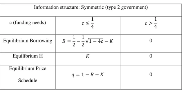
Table 2 : Market equilibrium under symmetric information and type 2 Information structure: Symmetric (type 2 government)
c (funding needs) 𝑐 ≤1 4 𝑐 > 1 4 Equilibrium Borrowing 𝐵 =1 2− 1 2√1 − 4𝑐 − 𝐾 0 Equilibrium H 𝐾 0 Equilibrium Price Schedule 𝑞 = 1 − 𝐵 − 𝐾 0
22 Expected payoff Government 1 4+ 1 4√1 − 4𝑐 − 𝑐 2 0 Lenders’ expected profit 0 0 Default probability 1 2− 1 2√1 − 4𝑐 0
3.2.3 Equilibrium under asymmetric information about type
In this section, I introduce the information friction, in the form of private type, that is, lenders do not know which government type they face when offering prices. This is meant to formalize the uncertainty regarding the level of transparency of countries’ borrowing data, after the Greek revelations. By solving the problem under asymmetric information, it is possible to draw conclusions about the information sensitivity of this market and the resulting impact on welfare.
Definition 1: Asymmetric information about type consists of lenders believing that the
government is of type 1 with probability 1 − 𝑃 and of type 2 with probability 𝑃. The timing of the game is now the following:
A. Decision problem of the government
At 𝑡 = 0, a type 1 government chooses 𝐵 to maximize its lifetime expected payoff: max 𝐵 𝑦0− 𝑐 + 𝑞𝐵 + ∫ (0)𝑑𝐹(𝑦1) + ∫ (𝑦1− 𝐵)𝑑𝐹(𝑦1) 1 𝐵 𝐵 0
At 𝑡 = 0, taking 𝐵 as given, a type 2 chooses 𝐻 = 𝐾 if and only if (and 𝐻 = 0 otherwise):
Government announces B Investors offer discount price Government chooses H Period 1 income is realized Government repays or defaults Government enjoys income
23 max 𝐵 𝑦0− 𝑐 + 𝑞 ∗ (𝐵 + 𝐾) + ∫ 0𝑑𝐹(𝑦1) + ∫ (𝑦1− (𝐵 + 𝐾))𝑑𝐹(𝑦1) 1 𝐵+𝐾 𝐵+𝐾 0 > max 𝐵 𝑦0− 𝑐 + 𝑞 ∗ (𝐵) + ∫ 0𝑑𝐹(𝑦1) + ∫ (𝑦1− (𝐵))𝑑𝐹(𝑦1) 1 𝐵 𝐵 0
And chooses 𝐵 to maximize its lifetime expected payoff, taking 𝐻 as given: max 𝐵 𝑦0− 𝑐 + 𝑞 ∗ (𝐵 + 𝐻) + ∫ 0𝑑𝐹(𝑦1) + ∫ (𝑦1− (𝐵 + 𝐻))𝑑𝐹(𝑦1) 1 𝐵+𝐻 𝐵+𝐻 0
B. Equilibrium bond price
Since a type 2’s choice of 𝐻 is optimally binary (either 0 or K) and since pricing 𝐻 = 0 makes it optimal for a type 2 to choose 𝐻 = 𝐾, which is cannot be an equilibrium (lenders would be making a loss), a necessary condition for the equilibrium price is that it assumes that a type 2 chooses H=K. So, in equilibrium, lenders’ payoff must be:
𝐸(𝜋) = −𝑞𝐵 + 𝑃(𝐵(1 − 𝐵 − 𝐾)) + (1 − 𝑃)(𝐵(1 − 𝐵))
The risk of default is the risk of default of a type 1 with probability (1-P) and that of a type 2, with probability P. Equating expected profits to zero yields the following price schedule:
𝑞 = 1 − 𝐵 − 𝑃𝐾
Intuitively, if lenders are uncertain about the government’s ability to hide debt, they are willing to incur in a loss in case the government can indeed hide debt, as long as they incur in a profit, in case the government cannot hide debt. The price is unfairly low to a well-behaved government and unfairly high to a bad government. If a new lender lowers the discount price, the government will not prefer her loans, since the revenues per unit of debt are lower. If a new lender increases the discount price, she will make an expected loss, since a type 2 will continue to borrow K. So this is a Nash-equilibrium.
C. Equilibrium lending
This price schedule can implement a pooling equilibrium, in which a type 2 does not reveal its type (hence the equilibrium is consistent with lenders belief 𝑃) and hides 𝐾 (hence the price
24 schedule achieves zero expected profits) if and only if it is IC for a type 2. For a type 2, it is incentive-compatible to hide 𝐾 if the price is sufficiently high. Hence, a type 2 chooses 𝐻 = 𝐾 and not 𝐻 = 0 if and only if:
max 𝐵 𝑦0− 𝑐 + 𝑞 ∗ (𝐵 + 𝐾) + ∫ 0𝑑𝐹(𝑦1) + ∫ (𝑦1− (𝐵 + 𝐾))𝑑𝐹(𝑦1) 1 𝐵+𝐾 𝐵+𝐾 0 > max 𝐵 𝑦0− 𝑐 + 𝑞 ∗ (𝐵) + ∫ 0𝑑𝐹(𝑦1) + ∫ (𝑦1− (𝐵))𝑑𝐹(𝑦1) 1 𝐵 𝐵 0 At a price schedule of 𝑞(𝐵) = 1 − 𝐵 − 𝑃𝐾
It can be shown that this only happens if 𝑃 <12. In that case, hiding is profitable, for which reason a type 2 will mimic the choice of 𝐵 of a type 1 and not reveal information about its type. Therefore, the equilibrium 𝐵 for both types solves:
max 𝐵 −𝑐 + 𝑞𝐵 + ∫ 0𝑑𝐹(𝑦1) + ∫ (𝑦1− 𝐵)𝑑𝐹(𝑦1) 1 𝐵 𝐵 0 𝑠. 𝑡. 𝑞𝐵 ≥ 𝑐 𝑞(𝐵) = 1 − 𝐵 − 𝑃𝐾 𝐵 < 1 Which is 𝐵 =1 2(1 − 𝑃𝐾) − 1 2√(1 − 𝑃𝐾)2− 4𝑐
In order for this pooling equilibrium to hold, it must be IR for a type 1. The highest 𝑐 for which it is IR for a type 1 is defined by the price schedule, as usual. It is the maximum of the function 𝑞𝐵 at the price schedule 𝑞(𝐵) = 1 − 𝐵 − 𝑃𝐾, which yields 𝑐 <14− 𝑃𝐾 (2−𝑃𝐾4 ).
Hence, for 𝑐 < 14− 𝑃𝐾 (2−𝑃𝐾4 ), the market is in a pooling equilibrium, in which both types borrow the same amount of 𝐵 and a type 2 borrows 𝐾. The well-behaved government ends up
25 paying a rent (through the market price) to a type 2 in order to be able to participate in the market.
For 𝑐 >14− 𝑃𝐾 (2−𝑃𝐾4 ), this equilibrium is not IR for a type 1, since the price schedule becomes negative, but it might be IR for a type 2, since it can make the price of 𝐵 positive at the prevailing price schedule, by decreasing the demand for 𝐵 and borrow 𝐾. However, it will signal its type and lenders would adapt the price schedule to a type 2. As a result, when 𝑐 >
1
4− 𝑃𝐾 ( 2−𝑃𝐾
4 ), lenders offer 𝑞(𝐵) = 1 − 𝐵 − 𝐾, there is market breakdown for a type 1
government and a type 2 chooses 𝐵 to solve the same problem as with symmetric information:
max 𝐵 𝑦0− 𝑐 + 𝑞 ∗ (𝐵 + 𝐾) + ∫ 0𝑑𝐹(𝑦1) + ∫ (𝑦1− (𝐵 + 𝐾))𝑑𝐹(𝑦1) 1 𝐵+𝐾 𝐵+𝐾 0 𝑠. 𝑡. 𝑞(𝐵 + 𝐾) ≥ 𝑐 𝑞(𝐵) = 1 − 𝐵 − 𝐾 𝐵 + 𝐾 < 1 Whose solution is:
𝐵 =1 2−
1
2√1 − 4𝑐 − 𝐾 𝐻 = 𝐾
The only lending equilibrium is then a separating equilibrium in which there is adverse selection, since only a type 2 participates in the market. A type 2 will participate up to 𝑐 < 14, which the is the maximum amount of funds that can be raised in an equilibrium with symmetric information and a type 2.
If 𝑃 >12, this asymmetric information price schedule does not make hiding IC (the price is not sufficiently higher than the repayment probability of the loan to make borrowing payoff-increasing). In this case, there is no zero expected profits price that can induce a bad type into
26 choosing the behavior it should choose for that price, except for a low enough price which makes it non-IR for a type 1 to borrow.
So the only possible lending equilibrium is one in which lenders offer a price schedule that makes it IR to borrow only for a type 2. Hence, there is a separating equilibrium, in which there is adverse selection, since only a type 2 participates in the market. It is only possible to separate types if 𝑐 >14−12𝐾(1 −𝐾2), since only then is it not IR for a type 2 to borrow at a type 2 price schedule (𝑞 = 1 − 𝐵 − 𝐾). In this case, a type 2 will borrow 𝐵 and 𝐾 as in a symmetric equilibrium and will participate up to 𝑐 <14, which the is the maximum amount of funds that can be raised in an equilibrium with symmetric information and a type 2. These findings are summarized in Lemma 3.
Lemma 3: With asymmetric information about the government’s type, lending exists in
equilibrium for 𝑐 < 14− 𝑃𝐾 (2−𝑃𝐾4 ) for a type 1 and for 𝑐 <41 for a type 2, if 𝑃 <12. If 𝑃 >12, the market is in a zero lending equilibrium for any c for a type 1 and lending exists for 𝑐 >14−
1
2𝐾(1 − 𝐾
2) for a type 2.
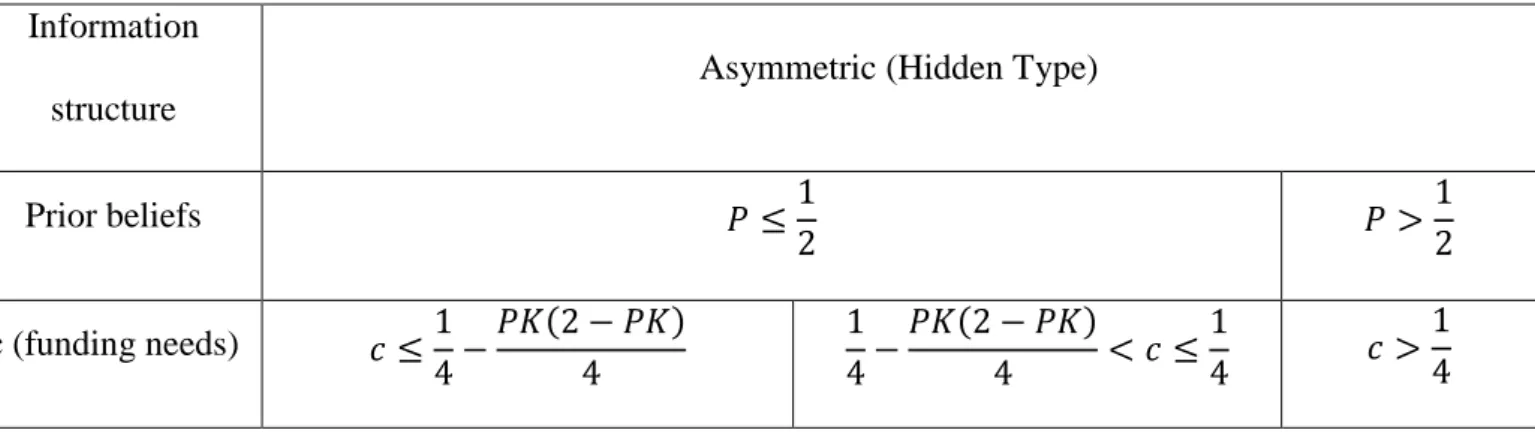
Table 3 describes the market equilibrium under asymmetric information, as a function of c: Table 3: Market equilibrium under asymmetric about type
Information structure
Asymmetric (Hidden Type)
Prior beliefs 𝑃 ≤ 1 2 𝑃 > 1 2 c (funding needs) 𝑐 ≤ 1 4− 𝑃𝐾(2 − 𝑃𝐾) 4 1 4− 𝑃𝐾(2 − 𝑃𝐾) 4 < 𝑐 ≤ 1 4 𝑐 > 1 4
27 Equilibrium Borrowing 𝑇𝑦𝑝𝑒 1 = 𝑇𝑦𝑝𝑒 2: 𝐵 = 1 2(1 − 𝑃𝐾) −1 2√(1 − 𝑃𝐾)2− 4𝑐 𝑇𝑦𝑝𝑒 1: 𝐵 = 0 𝑇𝑦𝑝𝑒 2: 𝐵 =1 2− 1 2√1 − 4𝑐 − 𝐾 𝑇𝑦𝑝𝑒 1 = 𝑇𝑦𝑝𝑒 2: 𝐵 = 0 Equilibrium Hidden borrowing 𝑇𝑦𝑝𝑒 1: 𝐻 = 0 𝑇𝑦𝑝𝑒 2: 𝐻 = 𝐾 𝑇𝑦𝑝𝑒 1: 𝐻 = 0 𝑇𝑦𝑝𝑒 1: 𝐻 = 𝐾 0 Equilibrium price schedule 𝑞 = 1 − 𝐵 − 𝑃𝐾 𝑞 = 1 − 𝐵 − 𝐾 𝑞 = 0 Expected payoff Government 𝑇𝑦𝑝𝑒1:1 4 +1 4(1 + 𝑃𝐾)√(1 − 𝑃𝐾)2− 4𝑐 −𝑐 2+ 𝑃2𝐾2 4 𝑇𝑦𝑝𝑒2:1 4 +1 4(1 + 𝑃𝐾)√(1 − 𝑃𝐾)2− 4𝑐 −𝑐 2+ 𝑃2𝐾2 4 + 𝐾2( 1 2− 𝑃) 𝑇𝑦𝑝𝑒1: 0 𝑇𝑦𝑝𝑒 2:1 4+ 1 4√1 − 4𝑐 − 𝑐 2 0 Average Expected payoff Government 1 4+ 1 4(1 + 𝑃𝐾)√(1 − 𝑃𝐾)2− 4𝑐 −𝑐 2+ 𝑃2𝐾2 4 + 𝑃𝐾2(1 2− 𝑃) 𝑃 (1 4+ 1 4√1 − 4𝑐 − 𝑐 2) 0 Lenders’ expected profit 0 0 0
28
3.3 Welfare
I use as measure of welfare the highest level of financing needs at which a government can be served in equilibrium. The higher such an upper bound, the higher the welfare provided by the equilibrium.
The government’s welfare increases with the opportunity to borrow in the market, because without borrowing the government defaults on its bills and cannot move on to the next period. In case the government defaults, it achieves a payoff of zero and does not have access to next period’s income, so his lifetime payoff is 0. On the contrary, if the government pays its bills, it can enjoy next period’s income. Although the government carries a debt burden into the next period, enforcement of loans is imperfect, which safeguards that the worst scenario for the government next period is to suffer the default cost of repudiating on its debt. Since default cost next period equals default cost this period (a payoff of 0), borrowing weakly dominates autarky. Lenders make zero expected profits in equilibrium independently of providing lending or not, so aggregate welfare in this economy is the welfare of the government.
When there is symmetric information about the government’s type, lending exists up to the point where imperfect enforcement allows it to exist. The ability to hide borrowing does not distort welfare if the government who can hide borrowing has a linear payoff function in consumption. In turn, asymmetric information about the government’s type distorts welfare. Overall, asymmetric information makes welfare incomparable when 𝑃 <12 (either higher or lower for a type 2, depending on the parameters, but certainly lower for a type 1) and dominated by symmetric information when 𝑃 > 12 (either no one is served or only type 2 is served). When there is asymmetric information about the government’s type, a government that can hide debt has advantages in doing so, if the price is sufficiently attractive. A government that can hide does not find it attractive to do it for every price. The price must be sufficiently higher that the repayment probability of its total loan (observed and hidden). This is so, because the
29 marginal cost of debt is higher than its repayment probability (since default is also costly). So the price must be sufficiently higher than the repayment probability of the loan to make the benefit of borrowing higher than its cost. This is the reason why, if a government cannot hide debt, the optimal amount of debt is the minimum necessary to satisfy the budget constraint. Since the marginal benefit of debt (the price) is its repayment probability and the marginal cost of debt is larger than its repayment probability, the optimal amount is the minimum necessary to allow the government to satisfy its budget constraint (the government only borrows, because borrowing is necessary to avoid default and enjoy next period’s income).
If lenders are uncertain about the government’s ability to hide debt, they are willing to incur in a loss in case the government can indeed hide debt, as long as they incur in a profit, in case the government cannot hide debt. The price is unfairly low to a well-behaved government and unfairly high to a bad government.
This asymmetric information price schedule makes hiding IC if the belief that the government is bad is lower than ½. In this equilibrium, a hiding government achieves a higher payoff than under symmetric information if the belief about being of the bad type is not too high and/or if financing needs are low enough. Indeed, although a bad type enjoys an unfairly high price, it also has to borrow an unnecessarily high amount of 𝐵 to mimic the behavior of a well-behaved type and keep its type private in this pooling equilibrium. Under a symmetric information equilibrium, a bad government optimally finances 𝑐 through both 𝐵 and 𝐾, whilst, in this equilibrium, it must finance 𝑐 entirely through 𝐵. Since the positive effect of a higher price is dominated by the negative effect of a higher 𝐵, having to pool is costly for a type 2. Hence, the welfare of a type 2 only increases with asymmetric information if the gain from hiding at a high price is higher than the cost of pooling. Formally, this happens when:
𝐾2(1 2− 𝑃) > 1 4√1 − 4𝑐 − 1 4(1 + 𝑃𝐾)√(1 − 𝑃𝐾)2− 4𝑐 − 𝑃2𝐾2 4
30 The left-hand-side is the gain from profitable hiding, which is the benefit form concealing its type. The right-hand-side is the cost of being in a pooling equilibrium, which is the price to pay to conceal its type. This inequality is satisfied if 𝑃 is sufficiently small (so that the decrease in the price schedule is small) or if 𝑐 is sufficiently low (so that the increase in 𝐵 is small). The welfare loss of a type 1 is the right-hand-side of the inequality.
Lenders are equally well off under symmetric and asymmetric information, since they make zero expected profits in both cases. The one who loses with asymmetric information for sure is a well-behaved government, since it ceases to be served by the market if financing needs are too high and since its payoff at any given level of financing needs at which it is served is lower. The well-behaved government ends up paying a rent to a type 2 in order to be able to participate in the market. When this rent is too high, it becomes unprofitable to participate in the market. So there are two distortions on welfare in this equilibrium: on the one hand, a type 1 pays a rent to a type 2 (pooling equilibrium). On the other, there are lost gains from trade, since a type 1 is excluded from the market for values of financing needs at which it participated in the market under symmetric information (separating equilibrium due to adverse selection). When type 1 is excluded from the market, a type 2 does not receive a rent from type 1 and it is as well off as it is under symmetric information. In this case, a type 1 loses welfare that is no one’s gain. If the belief that the government is bad is higher than ½, this asymmetric information price schedule does not make hiding IC (the price is not sufficiently higher than the repayment probability of the loan to make borrowing payoff-increasing). In this case, there is no zero expected profits price that can induce a bad type into choosing the behavior it should choose for that price, except for a low enough price which makes it non-IR for a type 1 to borrow. This is a separating equilibrium, which only serves a type 2. In conclusion, if the belief of a bad type is high enough (𝑃 >12), the effects are that there is no lending for low levels of financing needs
31 (market breakdown) and, for high levels of financing needs, there is adverse selection in a separating equilibrium where only a bad type borrows.
When 𝑃 <12, the binding constraint on the levels of financing needs at which the market provides lending to a well behaved government is the price schedule. Since the price schedule decreases with P and K (because P and K increase the risk of debt dilution) the higher P and the higher K, the lower the levels of financing needs at which a type 1 is still served by the market. The welfare of a type 2 in this pooling equilibrium is also decreasing in P, since it increases the cost of pooling, but, if P is sufficiently low, its welfare increases in K, since K increases the profit from hiding. These findings are summarized in Proposition 2.
Proposition 2:
If 𝑃 <12, asymmetric information about the government’s type induces a transfer of welfare from a type 1 government to a type 2. In this case, asymmetric information decreases the welfare of a type 1 and increases that of a type 2 only if P or c are sufficiently small.
If 𝑃 >12, asymmetric information decreases the welfare of a type 1 by ceasing to provide it with market lending and decreases the welfare of a type 2 by ceasing to provide it with market lending for low enough financing needs.
Under asymmetric information, when 𝑃 <12, a type 1’s welfare is decreasing in P and K, but a type 2’s welfare is decreasing in P and increasing in K if P is sufficiently low.
4. Chapter II: a mechanism of costly inspection and penalties for cheating
4.1 The model with the mechanism
In this section, I allow for inspection to be conducted by lenders through the payment of a fixed monitoring cost 𝑀 and assume that inspection reveals the amount of hidden borrowing. If a government is found cheating, that is, if 𝐻 = 𝐾, it has to pay a fixed penalty 𝑥 to lenders.
32 Since I interpret this mechanism as an official bailout, the zero expected profit requirement is not imposed by perfect competition, but rather by official lenders setting a fair return to capital. I will only focus on the problem of a type 2 government and on the problem of lenders. A type 1 government cannot hide, so its problem is the same as without the mechanism. Using the timeline of the game, I start in the moment where a type 2 government chooses to hide or not and use backward induction to compute the equilibrium of the market.
4.2 Equilibrium with commitment to inspect
When lenders make their inspection decision before granting the loan, the timeline is as follows:
A. The problem of a type 2 government
Since the government knows lenders’ inspection decision when deciding whether to hide, this game is sequential and its extensive form representation is depicted below:
At the time that a type 2 government makes its hiding decision, 𝐵 is a given. So, assuming that lenders decide to inspect (the left side of the tree), a type 2’s expected payoff if it hides is:
−𝑐 + 𝑞(𝐵 + 𝐾) + ∫ (0 − 𝑥)𝑑𝐹(𝑦1) 𝐵+𝐾 0 + ∫ [𝑦1− (𝐵 + 𝐾) − 𝑥]𝑑𝐹(𝑦1) 1 𝐵+𝐾
Its expected payoff if it does not hide is:
M ~M H ~H H ~H Lenders Type 2 Type 2 𝑦0 B q H Type 2 M 𝑦1 Default/repayment
33 −𝑐 + 𝑞(𝐵) + ∫ (0)𝑑𝐹(𝑦𝐵 1)
0
+ ∫ [𝑦1 1− (𝐵)]𝑑𝐹(𝑦1)
𝐵
Hence, a type 2 government hides if and only if the former is higher than the latter: −𝑐 + 𝑞(𝐵 + 𝐾) + ∫𝐵+𝐾(0 − 𝑥)𝑑𝐹(𝑦1) 0 + ∫1 [𝑦1− (𝐵 + 𝐾) − 𝑥]𝑑𝐹(𝑦1) 𝐵+𝐾 > −𝑐 + 𝑞(𝐵) + ∫ (0)𝑑𝐹(𝑦𝐵 1) 0 + ∫ [𝑦1 1− (𝐵)]𝑑𝐹(𝑦1) 𝐵
This yields the following condition on the penalty to induce a type 2 not to hide: 𝑥 = 𝐾 (𝐾
2− 𝑀
𝐵)
On the other side, if lenders decide not to inspect (the right hand side of the tree), the problem of a type 2 government is the one under asymmetric information without the mechanism.
B. Equilibrium bond price
Assuming that the penalty induces no-hiding, lenders’ payoff from inspection is: 𝐸(𝜋) = −𝑞𝐵 − 𝑀 + (1 − 𝐵)𝐵
And the bond price schedule is pinned down by equating lenders’ expected profit to 0: 𝑞 = 1 − 𝐵 −𝑀
𝐵
Assuming that the penalty does not deter hiding, lenders’ payoff from inspection is: 𝐸(𝜋) = −𝑞𝐵 − 𝑀 + 𝑃𝑥 + 𝑃(1 − 𝐵 − 𝐾)𝐵 + (1 − 𝑃)(1 − 𝐵)𝐵 And the bond price schedule is pinned down by equating lenders’ expected profit to 0:
𝑞 = 1 − 𝐵 − 𝑃𝐾 −𝑃𝑥 − 𝑀 𝐵
If lenders decide not to inspect, the equilibrium bond price is the no mechanism price schedule: 𝑞 = 1 − 𝐵 − 𝑃𝐾
C. Equilibrium lending
There are two possible equilibria by introducing the mechanism. In Equilibrium 1, lenders inspect and a type 2 government does not hide. In this equilibrium, the penalty is strong enough
34 to correct incentives to hide. Since it does not hide, lenders do not benefit from the penalty and must price in the monitoring cost in order to achieve zero expected profits. In Equilibrium 2, lenders inspect and a type 2 hides. In this case, the penalty is not strong enough to correct incentives to hide. However, in this case lenders extract a penalty from type 2 ex post. Hence, in Equilibrium 2, the price schedule of loans reflects not only the monitoring cost, but also a spread to cover for debt dilution risk (since a type 2 hides) and the prospect of receiving the penalty. Equilibrium 1 and 2 can coexist for the same levels of financing needs. The one that provides lending for the highest level of financing needs depends on the values of the parameters and is influenced by how the level of financing needs affects incentives to hide. In Equilibrium 1, incentives to hide increase with the level of financing needs, while, in Equilibrium 2, they decrease. Although the first-order effects of c on the benefit and cost of hiding cancel each other out in the two equilibria (both are the probability of default), the second-order effect of c on the cost of hiding is null in both equilibria, but its effect on the benefit of hiding is positive in Equilibrium 1, since c decreases the negative effect of M on the price and it negative in Equilibrium 2, since c decreases the positive effect of the inspection profit on the price. As such, Equilibrium 2 holds only if financing needs are low, since for high levels of financing needs, hiding becomes unprofitable for a type 2, which is not an equilibrium strategy. In turn, when the inspection cost and the penalty are both low, Equilibrium 1 holds also only for low levels of financing needs, since for high levels of financing needs hiding becomes profitable. As a result, Equilibrium 1 provides lending for higher values of financing needs provided that the penalty and the inspection cost are not too low, except when the penalty is sufficiently high and the inspection cost is sufficiently low, since the price under Equilibrium 2 would benefit substantially from the expected profit from inspection. The remainder of this sub-section is technical and describes both equilibria.
35 max 𝐵 𝑦0− 𝑐 + 𝑞 ∗ (𝐵) + ∫ 0𝑑𝐹(𝑦1) + ∫ (𝑦1− (𝐵))𝑑𝐹(𝑦1) 1 𝐵 𝐵 0 𝑠. 𝑡. 𝑞𝐵 ≥ 𝑐 𝑞(𝐵) = 1 − 𝐵 −𝑀 𝐵 Both government types borrow:
𝐵 =1 2−
1
2√1 − 4(𝑀 + 𝑐) And a type 2 chooses 𝐻 = 0.
Introducing the equilibrium amount of 𝐵 on the constraint that the penalty deters hiding at the prevailing market price implies that the following condition must be satisfied in equilibrium:
2𝑀𝐾 > (1 2−
1
2√1 − 4(𝑀 + 𝑐))(𝐾2− 2𝑥)
It can be shown that if 𝑀 > −2𝐾𝑥 +𝐾4, this condition is always satisfied. Otherwise, it imposes the following constraint on c:
𝑐 <1 4− 𝑀 − 1 4(1 + 4𝑀𝐾 2𝑥 − 𝐾2)2
Therefore, if 𝑀 > −2𝐾𝑥 +𝐾4, the constraint that the penalty is deterrent of hiding does not bind. In that case, since a type 2 does not hide in equilibrium, its payoff matches that of a type 1 and it is IR to borrow insofar as the bond market allows default in 𝑡 = 0 to be avoided. Hence, the binding constraint on c is the price schedule. At the schedule 𝑞 = 1 − 𝐵 −𝑀𝐵, the function 𝑞𝐵 attains a maximum of 14− 𝑀, so lending exists for 𝑐 <14− 𝑀.
On the contrary, if 𝑀 < −2𝐾𝑥 +𝐾4, the constraint that hiding is deterred is binding and it imposes
a tighter ceiling on c: 𝑐 <14− 𝑀 −14(1 +2𝑥−𝐾4𝑀𝐾2)2. The intuition for this constraint to bind for 𝑀 < −𝑥2𝐾+𝐾4 is the following: in this equilibrium, hiding is deterred both by M (which decreases
36 the benefit of hiding through the price) and by x (which increases the cost of hiding). Since incentives to hide are increasing in c under the commitment mechanism, if both M and x are high enough (𝑀 >−𝑥2𝐾+𝐾4), the inspection cost and the penalty are high enough to make hiding unprofitable for any positive value of c (there is no value of c that makes the benefit of hiding higher than its cost). When M and x are low (𝑀 < −𝑥2𝐾+𝐾4), the price and the penalty are not high enough to make hiding unprofitable for any c. Only for 𝑐 < 14− 𝑀 −14(1 +2𝑥−𝐾4𝑀𝐾2)2 is the
cost of hiding higher than its benefit for x and M such that 𝑀 <−𝑥2𝐾+𝐾4.
In Equilibrium 2, lenders inspect, but the penalty does not deter hiding, so a type 2 government hides. In that case, the equilibrium (𝑞, 𝐵, 𝐻) is the solution to:
max 𝐵 𝑦0− 𝑐 + 𝑞 ∗ (𝐵 + 𝐾) + ∫ (0 − 𝑥)𝑑𝐹(𝑦1) + ∫ (𝑦1− (𝐵 + 𝐾 + 𝑥))𝑑𝐹(𝑦1) 1 𝐵 𝐵 0 𝑠. 𝑡. 𝑞𝐵 ≥ 𝑐 𝑞 = 1 − 𝐵 − 𝑃𝐾 −𝑃𝑥 − 𝑀 𝐵 Both government types borrow:
1
2(1 − 𝑃𝐾) − 1
2√(1 − 𝑃𝐾)2− 4𝑐 + 4(𝑃𝑥 − 𝑀) And a type 2 chooses 𝐻 = 𝐾.
Introducing the equilibrium amount of 𝐵 on the constraint that the penalty does not deter hiding at the prevailing market price implies that the following condition must be satisfied:
𝑐 <1 4− 𝑀 − 1 4(1 − 2(1 − 𝑃𝐾) ( 4𝑃𝐾𝑥 − 4𝐾𝑀 2𝑥 − 𝐾2+ 2𝑃𝐾2) + ( 4𝑃𝐾𝑥 − 4𝐾𝑀 2𝑥 − 𝐾2+ 2𝑃𝐾2) 2 ) + 𝑃𝑥
The intuition for this upper bound on c is that, in this equilibrium, incentives to hide are decreasing in c, since the second order effect of c on the price (through B) is negative. That is
37 the case, because a higher c decreases the per unit (of B) profit that comes from extracting a penalty from type 2. Therefore, since a type 2 hides in equilibrium, c cannot be too high. Moreover, if 𝑃𝑥 > 𝑀, the following condition must be met: 𝑥 > 𝐾2 1−2𝑃2 . If 𝑃𝑥 < 𝑀, the following condition must be satisfied: 𝑥 < 𝐾2 1−2𝑃
2 .
Without inspection, the lending equilibrium is the one without the mechanism. Existence of Equilibria 1 and 2 are summarized in Lemma 4:
Lemma 4: With a mechanism in which lenders commit to inspect the government, lending exists
in equilibrium for 𝑐 < 𝑐′ for both government types, where:
𝑐′=1 4− 𝑀 if 𝑀 > 𝐾 4 − 𝑥 2𝐾 𝑐′=1 4− 𝑀 − 1 4(1 + 4𝐾𝑀 2𝑥−𝐾2) 2 if 𝑀 <𝐾4 −2𝐾𝑥
in an equilibrium in which lenders inspect and a type 2 government does not hide (Equilibrium 1) 𝑐′=1 4− 𝑀 − 1 4(1 − 2(1 − 𝑃𝐾) ( 4𝑃𝐾𝑥−4𝐾𝑀 2𝑥−𝐾2+2𝑃𝐾2) + ( 4𝑃𝐾𝑥−4𝐾𝑀 2𝑥−𝐾2+2𝑃𝐾2) 2 ) + 𝑃𝑥 if 𝑀 < 𝑃𝑥 and 𝑥 >𝐾22(1 − 2𝑃) or if 𝑀 > 𝑃𝑥 and 𝑥 <𝐾22(1 − 2𝑃)
in an equilibrium in which lenders inspect and a type 2 government hides (Equilibrium 2)
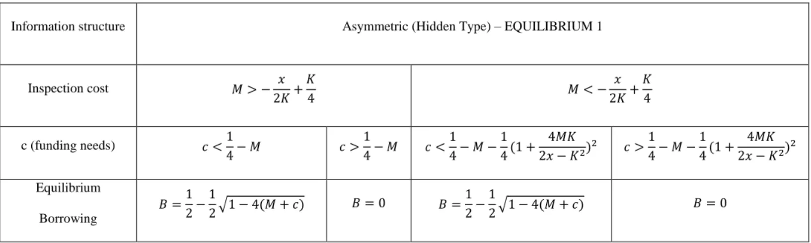
Tables 4 and 5 describe the market equilibrium as a function of c.
Table 4: Market equilibrium 1 under commitment mechanism
Information structure Asymmetric (Hidden Type) – EQUILIBRIUM 1
Inspection cost 𝑀 > − 𝑥 2𝐾+ 𝐾 4 𝑀 < − 𝑥 2𝐾+ 𝐾 4 c (funding needs) 𝑐 <1 4− 𝑀 𝑐 > 1 4− 𝑀 𝑐 < 1 4− 𝑀 − 1 4(1 + 4𝑀𝐾 2𝑥 − 𝐾2)2 𝑐 > 1 4− 𝑀 − 1 4(1 + 4𝑀𝐾 2𝑥 − 𝐾2)2 Equilibrium Borrowing 𝐵 =1 2− 1 2√1 − 4(𝑀 + 𝑐) 𝐵 = 0 𝐵 = 1 2− 1 2√1 − 4(𝑀 + 𝑐) 𝐵 = 0
38 Equilibrium price schedule 𝑞 = 1 − 𝐵 −𝑀 𝐵 𝑞 = 0 𝑞 = 1 − 𝐵 − 𝑀 𝐵 𝑞 = 0 Optimal Hidden borrowing 0 0 0 0 Expected payoff Government 1 4+ 1 4√1 − 4(𝑀 + 𝑐) − 𝑐 2− 𝑀 2 0 1 4+ 1 4√1 − 4(𝑀 + 𝑐) − 𝑐 2− 𝑀 2 0 Lenders’ expected profit 0 0 0 0
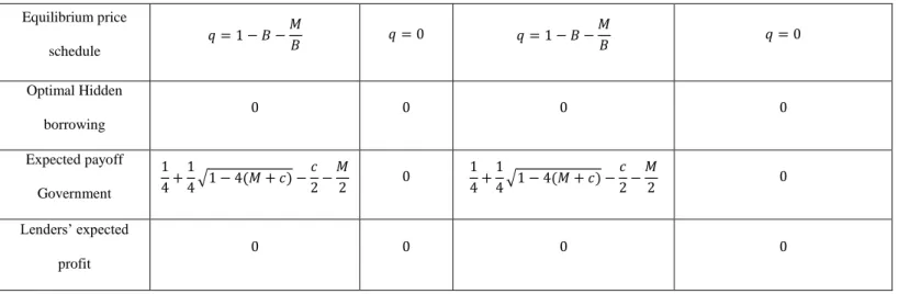
Table 5: Market equilibrium 2 under commitment mechanism
Information structure
Asymmetric (Hidden Type) – EQUILIBRIUM 2
Prior beliefs 𝑃 >1 2 𝑃 > 1 2 Inspection cost 𝑀 < 𝑃𝑥 𝑀 > 𝑃𝑥 𝑀 < 𝑃𝑥 and 𝑥 > 𝐾2 2(1 − 2𝑃) 𝑀 > 𝑃𝑥 and 𝑥 < 𝐾2 2(1 − 2𝑃) elsewhere
c (funding needs) 𝑐 < 𝑐′ Any 𝑐 < 𝑐′ 𝑐 < 𝑐′ Any
Equilibrium Borrowing 𝐵 =1 2(1 − 𝑃𝐾) −1 2√(1 − 𝑃𝐾)2− 4𝑐 + 4(𝑃𝑥 − 𝑀) 𝐵 = 0 𝐵 =1 2(1 − 𝑃𝐾) −1 2√(1 − 𝑃𝐾)2− 4𝑐 + 4(𝑃𝑥 − 𝑀) 𝐵 =1 2(1 − 𝑃𝐾) −1 2√(1 − 𝑃𝐾)2− 4𝑐 + 4(𝑃𝑥 − 𝑀) 𝐵 = 0 Equilibrium price schedule 𝑞 = 1 − 𝐵 − 𝑃𝐾 −𝑀 𝐵+ 𝑃𝑥 𝑞 = 0 𝑞 = 1 − 𝐵 − 𝑃𝐾 − 𝑀 𝐵+ 𝑃𝑥 𝑞 = 1 − 𝐵 − 𝑃𝐾 − 𝑀 𝐵+ 𝑃𝑥 𝑞 = 0 Optimal Hidden borrowing 𝑇𝑦𝑝𝑒 2: 𝐻 = 𝐾 𝐻 = 0 𝑇𝑦𝑝𝑒 2: 𝐻 = 𝐾 𝑇𝑦𝑝𝑒 2: 𝐻 = 𝐾 𝐻 = 0 Expected profit Government 𝑇𝑦𝑝𝑒 1:1 4 +1 4(1 − 𝑃𝐾)√(1 − 𝑃𝐾)2− 4𝑐 + 4(𝑃𝑥 − 𝑀) +𝑃2𝐾2 4 − 𝑐 2+ 𝑃𝑥 − 𝑀 2 𝑇𝑦𝑝𝑒 2 = 𝑇𝑦𝑝𝑒 1 + 𝐾(𝑃𝑥 −𝑀 𝐵+ 𝐾( 1 2− 𝑃) 0 𝑇𝑦𝑝𝑒 1:1 4 +1 4(1 − 𝑃𝐾)√(1 − 𝑃𝐾)2− 4𝑐 + 4(𝑃𝑥 − 𝑀) +𝑃2𝐾2 4 − 𝑐 2+ 𝑃𝑥 − 𝑀 2 𝑇𝑦𝑝𝑒 2 = 𝑇𝑦𝑝𝑒 1 + 𝐾(𝑃𝑥 −𝑀 𝐵 + 𝐾(1 2− 𝑃) 𝑇𝑦𝑝𝑒 1:1 4 +1 4(1 − 𝑃𝐾)√(1 − 𝑃𝐾)2− 4𝑐 + 4(𝑃𝑥 − 𝑀) +𝑃 2𝐾2 4 − 𝑐 2+ 𝑃𝑥 − 𝑀 2 𝑇𝑦𝑝𝑒 2 = 𝑇𝑦𝑝𝑒 1 + 𝐾(𝑃𝑥 −𝑀 𝐵 + 𝐾(1 2 − 𝑃) 0
39
Lenders’ expected profit
0 0 0 0 0
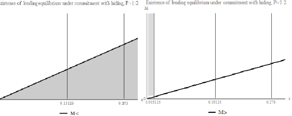
Figure 3: Parameter space of existence of commitment mechanism equilibrium 1
In the graph of Figure 3, K and P are fixed, M varies along the vertical axis and x varies along the horizontal axis. The shaded areas in the figure are the parameter values for which a lending equilibrium exists for a non-empty set of positive values of c. Different shades indicate different upper bounds on the set of values of c for which the lending equilibrium exists.
In the dark gray region, lending exists for 𝑐 <14− 𝑀. In the light gray region, lending exists for 𝑐 <14− 𝑀 −14(1 +2𝑥−𝐾4𝑀𝐾2)2. In the no-shade region, the set of positive values of c for which
lending exists is empty.
The upper bounds on c in each shaded region are determined by the constraint on c that binds in that region. In the dark gray region, the set of sustainable c is 𝑐 <14− 𝑀, because the binding constraint on the highest sustainable c is the price schedule. So, in the dark gray region, the highest sustainable c is negative for 𝑀 >14, it is 0 at 𝑀 =14 and it monotonically increases as M decreases, until 𝑀 = 0, where the highest sustainable c is 14. The derivative of the price with
Commitment deterring M M Commitment c 0 M
40 respect to the inspection cost is negative. If the inspection cost is too high, the spread charged for default risk plus the pricing in of the inspection cost per unit of debt are higher than the face value of debt and the price is negative. As the inspection cost decreases, the price increases, which increases the maximum of 𝑞𝐵 (price effect).
In the light gray region, lending exists for 𝑐 <14− 𝑀 −14(1 +2𝑥−𝐾4𝑀𝐾2)2, because the constraint
that hiding is deterred becomes binding. So, in the light gray region, the highest sustainable c is 0 when 𝑀 =14. As M decreases, the maximum sustainable c increases monotonically with M, until M reaches 𝑀 = −𝑥2𝐾+𝐾4 (the full line in Figure 3), where it discontinuously decreases from 𝑐 = 1 4+ 𝑥 2𝐾− 𝐾 4 to 𝑐 = 1 4+ 𝑥 2𝐾− 𝐾 4 − 1 4(1 + 4𝑀𝐾 2𝑥−𝐾2)2. As M decreases, 𝑐 = 1 4− 𝑀 − 1 4(1 + 4𝑀𝐾
2𝑥−𝐾2)2 does not vary monotonically with M. On the one hand, a lower M increases the
price schedule, which raises the funding ability at the prevailing price schedule (price effect). On the other hand, a lower M decreases the deterring effect of M, which lowers the maximum c for which hiding is deterred (incentives-to-hide effect). As a result, 𝑐 = 14− 𝑀 −
1 4(1 +
4𝑀𝐾
2𝑥−𝐾2)2 first increases as M decreases (price effect dominates), but, from 𝑀 = − 𝑥 2𝐾+ 𝐾
4 −
(2𝑥−𝐾2)2
8𝐾2 downwards, it decreases with M (incentives-to-hide effect dominates). When M
reaches 0, 𝑐 =14− 𝑀 −14(1 +2𝑥−𝐾4𝑀𝐾2)2 is 0, so lending is not restored for any positive c.
Figure 4: Parameter space of existence of commitment mechanism Equilibrium 2