Combining movement
and genetic data to
assess a forest
carnivore’s response to
forest fragmentation
André Lourenço
Mestrado de Biodiversidade, Genética e Evolução
Departamento de Biologia 2013
Orientador
Paulo Célio Alves, Professor Auxiliar, Faculdade de Ciências da Universidade do Porto
Coorientador
Todas as correções determinadas pelo júri, e só essas, foram efetuadas. O Presidente do Júri,
AGRADECIMENTOS
Em primeiro lugar, e como não poderia deixar de ser, agradeço aos meus orientadores professor Paulo Célio Alves e professor António Mira que providenciaram não só os meios logísticos sem os quais este trabalho não seria possível, mas também pelos conhecimentos fornecidos e sugestões que ajudaram a melhorar significativamente este manuscrito.
Gostaria de deixar também um agradecimento muito especial ao Filipe Carvalho que apesar de não ser oficialmente meu orientador, teve uma importância enorme neste trabalho ao fornecer os seus dados de telemetria da tese de doutoramento, pelos conhecimentos sobre genetas e também de análise estatística, e finalmente pelas suas sugestões que melhoraram significativamente a qualidade da minha tese.
Ao staff do CTM, em especial à Susana Lopes por toda a ajuda que disponibilizou na leitura de microsatélites e por todos os ensinamentos laboratoriais que transmitiu. Deixo também um agradecimento especial à Patrícia Ribeiro e à Filipa Martins por terem conseguido aturar-me durante um ano, ensinando-me as técnicas laboratoriais fundamentais para a execução deste trabalho.
Não poderia de deixar aqui uma nota especial ao Giovanni Manghi por toda a ajuda disponibilizada com softwares de Informação Geográfica, sendo crucial para executar as análises espaciais neste trabalho.
Ao pessoal do CIBIO que compareceu ao meu treino da apresentação, pelas sugestões efectuadas para melhorar a mesma que foram essenciais para aumentar a qualidade.
Como não poderia deixar de ser, deixo um agradecimento muito especial aos meus amigos pelo seu companheirismo, bom humor e com o qual passámos momentos espectaculares. Não irei estar a referir nomes em particular aqui porque esta secção ficaria enorme.
À minha família que tanto estimo, deixo um grande agradecimento pela sua presença na minha vida.
Aos meus irmãos, Manuela Lourenço, José Lourenço e Francisco Lourenço pelo companheirismo, pelas actividades e palhaçadas que costumamos fazer, pelas gargalhadas que partilhamos e também por alguns ensinamentos sobre a vida efectuados.
Finalmente, agradeço às pessoas mais importantes na minha vida, os meus pais. São eles os responsáveis por aquilo que sou hoje e sem eles não teria chegado até aqui.
RESUMO
A modificação de habitats naturais é atualmente reconhecido como uma grande ameaça à biodiversidade. A perda e a fragmentação dos habitats são reconhecidas como as principais causas da alteração da paisagem natural. Especificamente, a fragmentação do habitat modifica a configuração da paisagem, criando várias áreas de habitats desfavoráveis (matriz) para as espécies. A divisão de grandes e contínuas “manchas” em fragmentos mais pequenos rodeados por habitat não favorável, provoca um decréscimo na conetividade ao longo de uma determinada área. Esta interrupção do movimento, entre outras consequências negativas, bloqueia o fluxo génico entre diferentes áreas. Posteriormente, este fenómeno vai conduzir a um aumento da consaguineidade e diminuição da diversidade genética populacional entre individuos na mesma população, aumento o risco de extinção. De modo a combater estes efeitos negativos, medidas de mitigação devem de ser implementadas. Para poderem ser eficientes, estas medidas devem de ser suportadas por uma investigação científica robusta, e o aparecimento de novas áreas de investigação tais como a genética da paisagem, podem ter um papel fundamental na biologia da conservação. Atualmente, paisagens Mediterrânicas são dominadas por sistemas agro-forestais, onde uma grande proporção da floresta Mediterrânica original foi transformada em campos agrícolas. Por isso, animais como carnívoros florestais podem ser particularmente afetados por estas mudanças. Para entender como é que o fluxo génico é moldado por determinados tipos de habitats, é importante determinar com precisão a resistência que estes oferecem. Neste estudo usaram-se dados de telemetria de geneta (espécie de hábitos florestais) previamente recolhidos no âmbito de outro estudo num sistema agro-florestal no sul de Portugal, para estimar uma função de seleção de recursos de modo a avaliar objetivamente os efeitos da paisagem na variação genética nesta população de genetas. Foram colocadas três hipóteses fundamentais: (1) os dados de telemetria revelariam que as genetas usam mais zonas florestais comparativamente com outros tipos de habitats; (2) dados de parentesco e de movimento revelarão resultados discordantes relativamente aos efeitos da auto-estrada como barreira impermeável ao fluxo génico; e (3) modelos que assumem a heterogeneidade do habitat como um factor crucial que influencia a variação genética entre individuos serão mais suportados que modelos mais simplistas (por exemplo, modelos de isolamento por distância ou por barreira). Dezassete microsatélites foram genotipados com sucesso e com uma baixa taxa de erro para 74 amostras, de modo a estimar as distâncias genéticas entre os indivíduos amostrados. A equação calculada por uma regressão logística condicional revelou resultados do uso de habitats que são semelhantes àqueles obtidos por estudos anteriores, demonstrando que as genetas selecionam positivamente áreas com grande disponibilidade de recursos ecológicos (florestas de montado e galerias ripícolas) e evitaram significativamente zonas agrícolas e zonas próximas de perturbação humana. Apesar de a auto-estrada limitar os movimentos (de acordo com dados de telemetria),
esta população particular não sofreu subestruturação genética, provavelmente devido à recente construção desta barreira, não dando tempo suficiente para a população responder geneticamente. Contrariamente às expetativas iniciais, o modelo de isolamento por distância foi mais suportado do que modelos alternativos, apesar de apresentar baixos valores de correlação (Mantel r=-0.07; p<0.001). A agregação de grande parte das amostras recolhidas numa zona de habitat favorável relativamente contínuo provavelmente afectou a robustez deste modelo. O facto de as amostras estarem próximas espacialmente (aumentando a probabilidade de os indivíduos serem aparentados) numa zona favorável, não há grandes variações a nível genético entre os indivíduos nessa zona particular de amostragem. Isto implica que as diferentes variáveis de habitat consideradas estarão mal representadas nos cálculos das distâncias ecológicas entre diferentes indivíduos. Dessa forma, nessa zona altamente favorável aonde a maioria das amostras foram recolhidas, é provável que o fator principal que influencia a variação genética seja a distância geográfica. Para além disso, o papel que as galerias ripícolas desempenham como corredores de dispersão numa matriz desfavorável habitats desfavoráveis e limitações relacionadas com as técnicas de modelação usadas neste estudo, poderão ter tido alguma influência nos resultados obtidos. Melhorar a metodologia usada aqui no futuro, através da consideração de escalas espaciais e temporais apropriadas e que descrevem realisticamente processos de conetividade de fluxo génico, serão fundamentais para obter resultados mais robustos. É bastante importante ter isto em conta, para as autoridades de conservação no futuro atuarem de modo a reduzir os efeitos de fragmentação em espécies Mediterrânicas.
Palavras-chave: conetividade da paisagem; função de seleção de recursos; genética da paisagem; Genetta genetta; isolamento por resistência.
ABSTRACT
Landscape modification is actually recognized as major threat to biodiversity. Habitat loss and habitat fragmentation per se are acknowledged as the main negative consequences caused by landscape changes. Especially, habitat fragmentation modify landscape configuration, creating several areas of lower quality (matrix). The division of large continuous patches into smaller habitat patches surrounded by a low permeable matrix, greatly disturbs connectivity across the landscape. This movement disruption, among other negative consequences, impedes gene flow across the landscape. Eventually, this phenomenon will lead populations to inbreeding depression and loss of genetic diversity, reducing overall population fitness. In order to counteract these negative effects, conservation measures should be implemented. Nevertheless, accurate measures should be supported by solid scientific knowledge, and new research fields, like the landscape genetics prove to play an important role in conservation. Currently, Mediterranean landscapes are dominated by agro-forestry systems, where a great proportion of the original Mediterranean forest was transformed into agricultural fields. Therefore, genetic connectivity of several forest specialists, such as forest carnivores, may be particularly affected by these landscape changes. To understand the role of specific landscape features in shaping gene flow, it is fundamental to accurately quantify the resistance that these features impose to gene flow. Here, taking advantage of previously radio-tracking data collected for common genets (which are forest species) in an agro-forestry system in southern Portugal, a resource selection function (RSF) was estimated to objectively assess how landscape variables influenced genetic relatedness. Here, three hypotheses were tested: (1) radio-tracking data will reveal that common genets use more forested areas when compared with other types of habitats; (2) parental analysis and movement data will not present concordant results; and (3) models which assume habitat heterogeneity as a crucial factor that influences genetic variation between individuals will be more statistically supported than simpler models (for example, isolation-by-distance and isolation-by-barrier models). Seventeen microsatellites were successfully genotyped with low genotyping error rates for 74 samples, in order to estimate genetic relatedness between individuals. The conditional logistic regression equation calculated in the RSF was in accordance with previous studies, demonstrating that common genets select positively areas with high availability of ecological resources (montado forests and riparian corridors) and avoided agricultural fields and areas near human disturbance. Despite the highway disrupt movements (accordingly with radio-tracking data), this particular population is not genetically substructured probably due to the recent construction of this feature. Thus, the population did not have enough time to respond to the construction of the highway. Contrary to the initial hypotheses, the IBD (isolation-by-distance) model was more supported than the competing models, despite presenting low correlation values (Mantel r=-0.07; p<0.001). Most samples are clustered (non-random sampling) in a small region holding suitable contiguous habitat
which probably hampered the analyses. Since these samples are spatially close (increasing the probability of familiar relationships) in a favourable area, there are not great variations at the genetic level between individuals in that particular sampled zone. This implies that the different landscape features that were analysed are poorly represented in ecological distances calculations between individuals. Thus, in that particular region the geographical distance is probably the main factor influencing gene flow. Additionally, the role that riparian corridors may play as dispersal enhancers in unsuitable habitats and limitations concerning the modelling techniques used here, may have also contributed for the observed results. Refining the methodology employed here in the future, by accounting spatial and temporal scales that likely describe more realistically how processes responsible for genetic connectivity operate, is fundamental to obtain more robust results. This is very important, if conservation authorities want to reduce the effects of fragmentation in Mediterranean species in a near future..
Keywords: landscape connectivity; resource selection function; landscape genetics; Genetta genetta; isolation-by-resistance.
TABLE OF CONTENTS
AGRADECIMENTOS ... i
RESUMO ... iii
ABSTRACT ... v
TABLE OF CONTENTS ... vii
LIST OF FIGURES ... ix
LIST OF TABLES ... x
LIST OF ABBREVIATIONS ... x
1-INTRODUCTION ... 1
1.1- Landscape modification and its effects on biodiversity ... 1
1.2-Maintaining landscape connectivity ... 2
1.2.1-Overview ... 2
1.2.2-Landscape genetics as a tool to assess landscape functional connectivity ... 4
1.3-Study species ... 9
1.4-Objectives and hypotheses ... 12
2-METHODS ... 14
2.1-Study area ... 14
2.2-Sample collection for genetic analysis ... 15
2.3-Laboratory procedures ... 17
2.3.1-Marker selection ... 17
2.4-Microsatellite data analyses ... 21
2.5-Spatial analyses ... 23
2.5.1-Environmental spatial variables ... 23
2.5.2-Resource selection function ... 24
2.5.3-Landscape genetics analyses ... 27
3-RESULTS ... 29
3.1-Samples and microsatellites variability ... 29
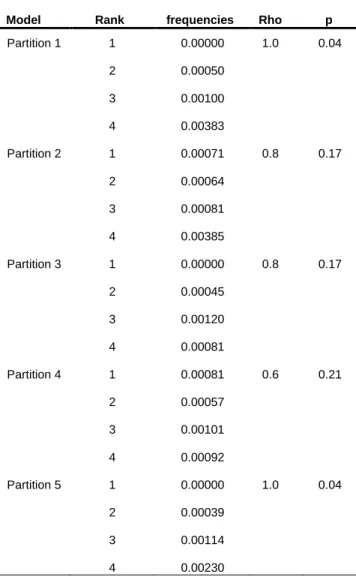
3.2-Model selection and validation ... 30
3.3-Mantel and partial Mantel results ... 33
4-DISCUSSION ... 34
4.1-Microsatellite performance ... 34
4.2- Landscape genetics analyses ... 39
4.2.1-Best model and RSF validity ... 39
5-REFERENCES ... 47 6-SUPPLEMENTARY MATERIAL ... 68
LIST OF FIGURES
Fig.1- Genetta genetta adult individual. Picture downloaded from http://www.regiaodeleiria.pt/wp-content/uploads/2013/09/gineta.jpg.
Fig.2- Worldwide distribution of the common genet. Blue areas represent the native extent, being absent from central Africa and the Sahara desert. Red regions comprise the introduced range, being confined to Iberian Peninsula, southern region of France and northwest of Italia. Areas with olive colour correspond to zones where it is extinct.
Fig.3- Montado area, a common feature of agro-forestry systems in Mediterranean landscapes. Photo credit – Unit of Conservation Biology of University of Évora.
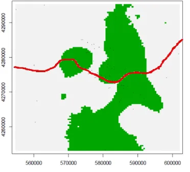
Fig.4- Home ranges near the highway are represented. It is possible to detect that some home ranges are bounded by the highway, indicating that this feature constitutes a behavioural barrier to movement.
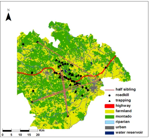
Fig.5- Study area with a total area of 2300 km2. Triangles represent samples obtained through cage-trapping, while circles correspond to samples gathered from road-killed animals. Five land cover classes are illustrated: yellow – agricultural fields; green – montado forest; dark blue – riparian ecosystems; grey – anthropogenic features; light blue – water reservoirs. The highway tested as a hypothetical barrier is also illustrated at red.
Fig.6- Sex identification of four samples in gel electrophoresis. Two females (1) and two males (2) are illustrated. In males, both genX5 and genY7 primers are amplified while in females only genX5 is amplified.
Fig.7- Representation of all parent/offspring and full sibling pairs estimated using COLONY. Note that related individuals are in different sides of the highway, revealing that the highway was successfully crossed probably during dispersal events. Purple lines connect related individuals. Fig.8- Representation of five half sibling relationships exhibiting the highest pairwise geographic distance. Pink lines connect individuals sharing half sibling relationships.
Fig.9- Suitability map constructed using conditional logistic equation form the top model. To facilitate map representation, each rank represents one quartile of probability of use (rank 1 – [0-0.25]; rank 2 – [0.26-0.50]; rank 3 – [0.51-0.75]; rank 4 – [0.76-1]). Greener areas are concordant with montado forests and riparian corridors.
Fig.10- Resistance map constructed using conditional logistic equation from the top model. Whiter areas present higher resistance values and are mainly correspondent to urban areas and roads. Darker areas represent suitable areas that have low resistance values such as montado forests and riparian corridors.
Fig.11- Current map created by Circuitscape for the IBR model. Dark blue areas represent higher values of current (i.e., areas highly permeable to movement) and lighter areas represent low values of current (i.e., with lower probability of being crossed by a random walker).
Fig.12- Current map created by Circuitscape for the IBD model. Dark blue areas represent higher values of current (i.e., areas highly permeable to movement) and lighter areas represent low values of current (i.e., with lower probability of being crossed by a random walker).
Fig.13- Estimated cluster membership in Geneland. X and Y axis represent UTM coordinates. Given that the highway cross the area in a west-east axis, it is visible by this figure that the population is not structured by the highway. Small black dots represent samples locations.
Fig.S1- Small portion of the study area illustrating the home ranges calculated for 21 genets. The home ranges that overlap belong to individuals from different sexes.
LIST OF TABLES
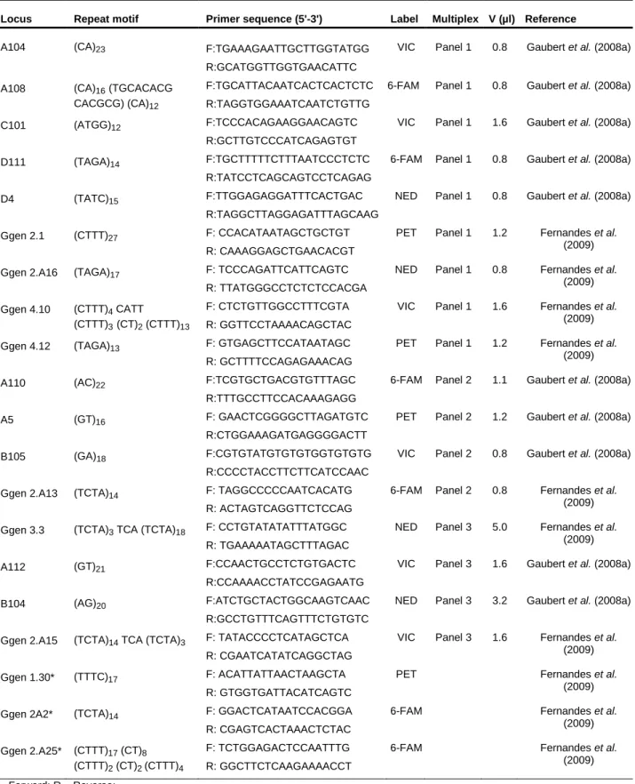
Table 1- Characterization of 20 microsatellite loci selected to genotype Genetta genetta samples. Information regarding repeat motif, primer sequence, optimized multiplex sets, fluorescent labels and the original reference where each marker was first published is also provided.
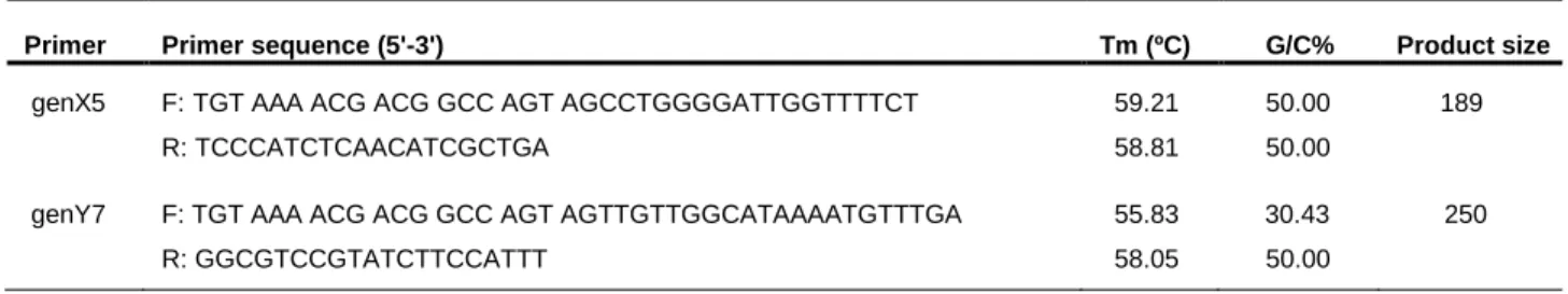
Table 2- Characterization of the re-designed primers for sexing genets.
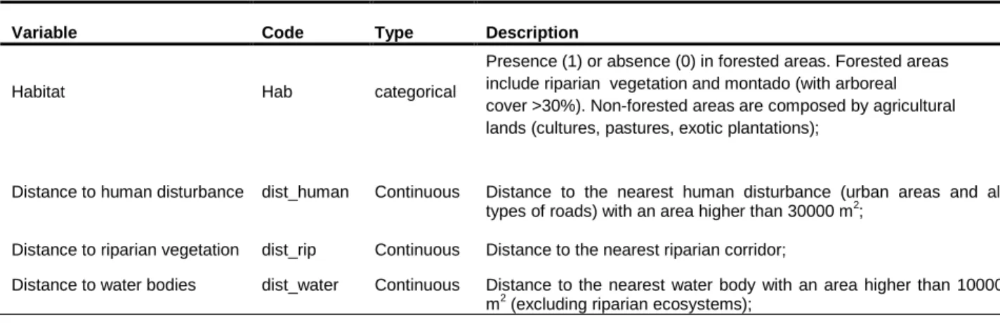
Table 3- Description of the landscape variables used in statistical analyses. The predictor set is constituted by one categorical variable (habitat) and three continuous variables (distance to human disturbance, distance to riparian vegetation and distance to water reservoirs).
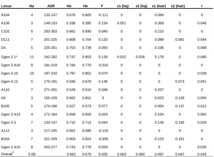
Table 4- Diversity measures and genotyping error rates from 17 microsatellites used in genetic analysis. Error rates from high quality samples and hair samples were calculated separately. Marker Ggen 2.1 was removed from all statistical analyses.
Table 5- Model ranking based on ∆AIC and Akaike weights (wi).
Table 6- Top model conditional logistic regression parameters.
Table 7- Model 5-fold cross validation using Spearman-rank correlation test (rho). Table 8- Mantel and partial Mantel correlation results.
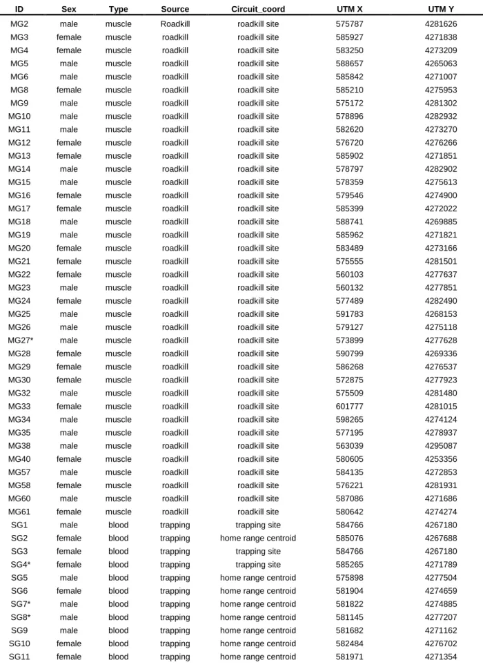
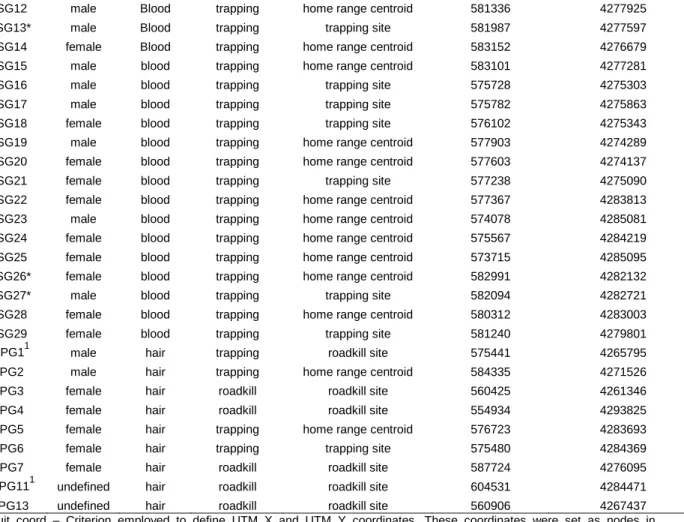
Table S1- Information regarding samples used in genetic analyses. It is included information about ID sample, sex, spatial coordinates, type and source of sample. Two samples were removed from genetic analyses.
Table S2- Spearman correlation matrix between the four predictive variables. Table S3- Variance inflation factors for each landscape variable.
LIST OF ABBREVIATIONS
AIC – Akaike Information Criterion LD – Linkage Disequilibrium FDR – False Discovery Rate
GIS – Geographical Information System HW – Hardy-Weinberg
IBB – Isolation-by-barrier IBD – Isolation-by-distance IBR – Isolation-by-resistance
ITA – Information Theoretic Approach LCP – Least Cost Path
MRDM- Multiple Regression on Distance Matrices PCR – Polymerase chain reaction
PIM – Population Inbreeding Model
rho – Spearman-rank correlation coefficient RSF – Resource Selection Function
RSPF – Resource Selection Probability Function VHF – Very High Frequency telemetry
1-INTRODUCTION
1.1- Landscape modification and its effects on biodiversity
Biodiversity decline is currently recognized as a major environmental concern issue. Landscape modification largely contributed for this decline, reducing habitat suitability quantitatively and qualitatively at both local and global scales (Foley et al. 2005; Fischer & Lindenmayer 2007). Agriculture, urbanization, forest clearing or construction of infrastructures greatly contributed for the transformation of pristine habitat into artificial or semi-natural landscapes over the last decades, causing major changes in habitat spatial structure (Foley et al. 2005; Hanski 2010). Hence, heterogeneous landscapes are created with smaller and isolated habitat patches embedded within a landscape matrix (unsuitable area surrounding favourable habitat patches for the species of interest) (Fahrig 2003; Fischer & Lindenmayer 2007). This landscape modification is mainly caused by two important phenomena – habitat loss and habitat fragmentation per se. Despite some initial issues to delimit the conceptual boundaries of both processes (Holt et al. 1995; Schumaker 1996), probably the best definitions are provided by Bender et al. (1998) and Fahrig (2003) (see also “dissection” phenomenon in Bogaert et al. 2004; Fischer & Lindenmayer 2007). Habitat loss consists on the removal of native vegetation, while habitat fragmentation per se (the expression “per se” means that the effects of pure habitat loss are controlled) is defined as the division of a contiguous patch into multiple smaller patches separated by a non-natural matrix. In other words, habitat loss changes patch size attributes and fragmentation interferes with spatial configuration of patches. Despite presenting different properties, both phenomena cannot be seen as fully independent (Bender et al. 1998; Wiegand et al. 2005). Usually fragmentation follows habitat loss, augmenting their effects. Thus, both threats must be taken into account jointly by conservation authorities.
Three major effects resultant from the combination of both above described processes can be observed. First, decrease of patch size (perceived as loss of native vegetation area) is the main and most serious negative impact, caused primarily by habitat loss (Fahrig 2001; Fahrig 2003; but see also Wiegand et al. 2005). Patch size reduction implies a loss of functional space, decreasing the available area to be used by species/individuals. Under these new conditions, intra- and interspecific interactions are altered and there is a decrease of food resources and shelter availability, ultimately leading to a higher mortality rate and lower breeding success (Fahrig 2003; Swift & Hannon 2010). Second, patch isolation mediated by habitat fragmentation is the main driver of connectivity disruption. Day-to-day movements, long migration routes or juvenile dispersal are negatively affected since the adjacent matrix (generally unsuitable) coerces individuals to stay in a particular patch or to travel through an inhospitable matrix, eventually increasing mortality risk (Ricketts 2001; Bender & Fahrig 2005; Bonte et al. 2012). Thus, if movement between patches is blocked then gene flow is also interrupted. The greater isolation experienced by individuals within
fragmented patches leads to inbreeding depression and loss of genetic diversity, reducing individual fitness and the ability for a particular population to adapt to environmental changes (Frankham 2005; Delaney et al. 2010; Struebig et al. 2011). Third, edge effects are expressed through changes of biotic (change in vegetation communities or alteration of species interactions such as competition or predation) and abiotic (such as microclimatic changes in insulation, moisture, wind patterns) conditions in the periphery of a patch (Murcia 1995; Ewers et al. 2007). The “new” boundary environment is generally hazardous for native species, reducing habitat quality and availability within a given area. These major threats can lead a population to a sharp decline, eventually reaching an irreversible critical threshold (also called extinction vortex) where environmental (eg: natural variation and catastrophic unpredictable events), genetic (eg: genetic drift) and demographic stochasticity (eg: natural oscilitation on yearly breeding success) acquire a significant importance as local drivers of extinction (Lande 1993; Dennis 2002; Blomqvist et al. 2010).
Taxa intrinsic features also play an important role on determining extinction proneness. Despite being processes transversal to many taxonomical groups (Andrén 1994; Didham et al. 1996; Andrews & Gibbons 2005; Aguilar et al. 2006), the particular combination of biological characteristics exhibited by each taxon will determine a differential susceptibility to landscape modification (Crooks 2002; Cushman 2006; see also table 2 in Fischer & Lindenmayer 2007). Mammalian carnivores constitute a clear example of vulnerability to habitat loss and fragmentation, and the biological traits that make them susceptible are relatively well known (Sunquist & Sunquist 2001; Crooks 2002; Boitani & Powell 2012). Carnivore populations usually present low densities and slow growth rates derived from low reproductive outputs. Moreover, large area requirements and other anthropogenic pressures (eg: hunting) constitute additional factors that inflate the deleterious effects of landscape changes on this group. The great dispersal ability shown by carnivores (usually more pronounced on juveniles or sub-adults) may counter-balance or exacerbate these consequences. Patch isolation effects may be minimized by being able to move through different patches, but on the other hand, high mobility may imply a greater willingness to travel through unsuitable habitat, increasing energy costs and mortality risk (Bonte et al. 2012).
1.2-Maintaining landscape connectivity
1.2.1-Overview
Counteracting landscape changes effects has been a major challenge for conservation authorities. To implement effective conservation measures, one must have knowledge about several landscape features such as patch size and isolation, characteristics of the surrounding matrix and ecological requirements of the target species (Fahrig 2003; Fischer & Lindenmayer 2007). Preventing fragmentation and habitat loss is probably the best solution to maximize
conservation efforts (Crooks & Sanjayan 2006). This is rarely accomplished and, in most situations, conservation authorities are faced already with post-disturbance scenarios. Restoring habitat quality and the original amount of area would be the ideal solution to this problem (Mortelliti et al. 2010; Brückmann et al. 2010; Hodgson et al. 2011). However, logistical and budget constraints hamper the viability of many conservation projects and alternative solutions must be considered in order to mitigate the loss of pristine habitat.
One viable option to reduce the fragmentation effects on species population (especially isolation effects) is to increase landscape connectivity between habitat patches. Landscape connectivity is defined as a context/species-specific concept that quantifies how movement of a particular entity (eg: pollen, seeds, genes, individuals or species) is facilitated on a particular environment (Crooks & Sanjayan 2006). The concept can be decomposed in two components: structural and functional (see review in Baguette et al. 2013). Structural connectivity describes the physic properties of the landscape such as the arrangement of patches, isolation degree and topography. Functional connectivity assesses the ecological and biological responses of a particular species or entity (individual, genes, seeds, etc.) to the structural characteristics of the landscape.
Studies focusing on landscape connectivity started to increase on early 1990’s, denoting the importance that this field acquired in conservation biology (Crooks & Sanjayan 2006). Complementary research fields such as metapopulation theory and landscape ecology, largely contributed for increasing the knowledge of important landscape processes (eg: matrix permeability, immigration patterns and dynamics of colonization and extinction patterns in patches) (Moilanen & Hanski 2006; Taylor et al. 2006). Additionally, development of GIS (Geographic Information System) and better modelling tools, as well the development of higher performance computers have allowed the generation of connectivity maps with finer resolution, contributing with more detailed information to researchers about spatio-temporal patterns of species response to fragmentation (Adriaensen et al. 2003; McRae 2006; Saura & Torné 2009).
During these last two decades, theoretical and empirical studies addressed the potential benefits of enhancing linkage between areas (Noss 1987; Beier & Noss 1998; Prevedello & Vieira 2010). Improving connectivity reduces movement costs (foraging movements, juvenile dispersal, migration), helps to prevent inbreeding depression, diminishes the risk of extinction in small isolated recipient populations and promotes ecological processes stability, such as natural disturbances, nutrient cycles or vegetation succession (Vilà et al. 2003; Crooks & Sanjayan 2006; Moilanen & Hanski 2006). Conversely, increasing connectivity in some situations can have biodiversity negative effects on biodiversity by promoting disease and exotic species spread and also can act as ecological traps, since they may increase exposure to several threats (eg: predator attraction) (Hess 1994; Crooks & Suarez 2006; McCallum & Dobson 2006). Outweighing the benefits and deleterious effects of such effort is a procedure that should be situation-specific; however, generally the advantages are obvious and cannot be disregarded. Despite its positive
effects on biodiversity, setting defragmentation measures into practice had lead to much controversy. Especially, corridor’s use and efficiency for maintaining long-term populations’ viability was questioned in the past (Simberloff et al. 1992; Beier & Noss 1998; Gilbert-Norton et al. 2010). The main criticisms concerned the small set of organisms that have been tested and the poorly implemented experimental designs (Beier & Noss 1998). However, Gilbert-Norton and colleagues (2010) on a review based on recent studies concluded, that in fact corridors are used by several species form different taxonomic groups. However, it is still not certain if corridors, as other conservation measures, such as stepping stone patches and management of sub-optimal matrix habitat (Fischer & Lindenmayer 2002; Baum et al. 2004; Prevedello & Vieira 2010) are efficient for maintaining long-term viability in populations (Hodgson et al. 2011). Improving not only modelling techniques, but also adopting robust management and assessment frameworks will enable scientists to effectively address connectivity issues. This is crucial to restore connectivity in fragmented landscapes.
1.2.2-Landscape genetics as a tool to assess landscape functional connectivity
Landscape functional connectivity can be measured through studies on individual movement behaviour (e.g. radio-telemetry) to assess landscape resistance to dispersal, migration and daily movements (Kindlmann & Burel 2008). Although these metrics give information about permeability to movement, they fail essentially in resolving one key aspect – they do not provide information concerning successful reproduction of migrants (Mills & Allendorf 1996; Vilà et al. 2003; Jaquiéry et al. 2011). To answer questions such as “Does a corridor enables enough gene flow to prevent inbreeding depression in the recipient isolated population?” or “Does a road creates population substructuring?”, the obvious approach is to gather information regarding gene flow. Hence, indirect gene flow assessment can act as surrogate measure of landscape permeability, providing at the same time information about genetic variability among subpopulations (Cushman et al. 2006; Pérez et al. 2009; Frantz et al. 2010). In order to help addressing these types of questions, the new research field of landscape genetics arose.
Following technological advances on molecular techniques, landscape genetics emerged as a promising research field tool that integrates landscape ecology, population genetics and spatial analyses. It is mainly concerned on investigating the impact of landscape features on species microevolutionary processes such as gene flow, genetic drift and adaptive genetic variation (Manel et al. 2003). The spatial and temporal scales involved on landscape genetics studies are smaller than other population genetic studies, such as phylogeography (Wang 2010). Thus, although holding a great potential to be applied to other research areas (Balkenhol et al. 2009), its applicability to address contemporary connectivity conservation issues has been recognized, leading to an increase of published papers on the last decade concerning this subject (Storfer et al.
2010). Landscape genetics statistics and its limitations have been addressed, leading to the improvement of spatial and genetic models employed at population and individual levels (Dyer et al. 2010; Cushman et al. 2013). All this research contributed for the establishment of a standard statistical framework. Basically, it comprises the correlation (eg: Mantel test, partial Mantel test) between pairwise (individual or populations) matrices of genetic and ecological distances (the term “effective distances” is also used in the literature) for the detection of genetic discontinuities and/or detection of the influence of particular landscape features on gene flow (eg: Coulon et al. 2004; Stevens et al. 2006; Graves et al. 2012). Following the causal modelling framework developed by Cushman et al. (2006), three types of models are usually tested: isolation-by-distance (IBD), isolation-by-barrier (IBB) and isolation-by-resistance (IBR). The only difference between the models relies on ecological distances calculations, since different distance metrics are employed (see below). The first two are considered as null hypotheses where correlation values are confronted with the alternative hypothesis represented by the IBR model. The latter is usually translated into several models that contain different combinations of landscape variables (Shirk et al. 2010; Garroway et al. 2011). In these tests, an adequate sampling that realistically describes the spatio-temporal processes operating in the landscape of interest, and additionally, the ability to accurately estimate genetic distances and ecological distances are crucial steps to robustly assess model performance.
The use of adequate molecular markers is the first step to obtain reliable differentiation measures between individuals or populations. In their review, Storfer and colleagues (2010) identified microsatellites (short tandem sequence repeats found in the nuclear genome) as the preferred molecular markers, at least in studies where the target species were animals (encompassing 70% of the reviewed papers). The fine temporal window (few to dozens of generations) that researchers face on landscape genetics studies requires markers with high mutation rates and hence, microsatellites constitute suitable candidates (Selkoe & Toonen 2006; Wang 2010). Genetic markers with higher mutation rates exhibit high allelic diversity within an evolutionary short period of time, retaining enough resolution to detect population microevolutionary responses to changes in landscape (Cushman et al. 2006; Garroway et al. 2011; Amos et al. 2012). Markers with lower mutation rates, such as sequences of mitochondrial and nuclear DNA, are more suitable to analyse events from a distant past such as the assessment of postglacial colonization genetic patterns or the evaluation of genetic isolation effects of a particular historical natural barrier (Shafer et al. 2010; Bryson et al. 2011). Despite their high resolution power, microsatellite genotyping is prone to a variety of errors such as: (1) the systematic non-amplification of an allele generally due to a point mutation on marker’s primer binding regions – null alleles; (2) allele stochastic amplification failure – allele dropout; and (3) allele misgenotyping due to human factors or to the generation of PCR artefacts Taq polymerase slippage on early cycles of PCR - false alleles (reviewed for example in Pompanon et al. 2005; Hoffman & Amos 2005; Selkoe
& Toonen 2006). Several factors can contribute to the increase of a particular type of errors (see table 2 in Pompanon et al. 2005). For example, low DNA quality and quantity is a common cause of allele dropout, constituting a relevant issue on non-invasive genetics (Waits & Paetkau 2005; Beja-Pereira et al. 2009; but see allele dropout for high quality samples in Soulsbury et al. 2007). Errors are inevitable and the best solution is to establish a solid quality control system, either on the laboratory procedures and on data analysis (Goossens et al. 1998; Piggott et al. 2004; Dakin & Avise 2004; Johnson & Haydon 2007; Chybicki & Burczyk 2009). Failure to account these errors may lead, among others, to a false increase on observed number of genotyped homozygotes (caused by null alleles and allele dropout), miscalculations of allelic frequencies and interference with Hardy-Weinberg and parentage analysis (Viard et al. 1998; Dakin & Avise 2004; Van Oosterhout et al. 2006; Johnson & Haydon 2007). Consequently, spurious scientific conclusions may be extrapolated. Landscape genetics studies rely heavily on a free bias genotyping to accurately estimate genetic distances between genetic units (eg: Pérez-Espona et al. 2008; Braunisch et al. 2010; Shirk et al. 2010). Phenomena such as null alleles or allele dropout, as stated above, lead to miscalculations of genetic distances and may obscure true marker polymorphism. Polymorphism is acknowledged as an important feature on this research field, providing more resolution power to microsatellites to detect landscape effects on genetic structuring (Holderegger & Wagner 2008; Wang 2010; Landguth et al. 2012). Thus, when theses errors are not taken into account, false landscape gene flow relationships can be obtained, having serious repercussions at conservation planning and management.
Calculation of ecological distance matrices for IBD and IBB models is straightforward. The IBD model simply assumes that genetic differentiation between individuals is only dependent of geographical distance (Wright 1943). Hence, the model predicts that one particular individual is more related with geographically closer individuals than the ones far apart. A pairwise distance (distance expressed in geographic or map cell units) matrix is then constructed and correlated with a pairwise matrix of genetic distances (eg: Murphy et al. 2010; Phillipsen & Lytle 2012; Quaglietta et al. 2013). The IBB model is used to test the effects of a particular barrier (eg: highway or a river) on gene flow (Cushman et al. 2006; Shirk et al. 2010). Panmixia on either side of the barrier with no gene flow between different sides of the barrier is assumed by the IBB model. No distance costs are considered between individuals on the same side of the barrier, while it is assigned a disproportionate maximum cost to cross the barrier. Hence, it is expected a higher relatedness among individuals on the same side of the barrier than among samples from different sides. These models are fairly unrealistic for most of the times. The IBD model assumes that an animal perceives the surrounding environment homogeneously. This is false for most species (see Frantz et al. 2010 for opposite results), since there is a hierarchical habitat selection where suitable habitats are selected over hostile environments (McRae 2006; Broquet et al. 2006). IBB model is also rather too simplistic since it disregards completely landscape features that may influence gene
flow, besides the barrier itself. Additionally, not all barriers constitute completely impermeable features (Coulon et al. 2006; Frantz et al. 2010). Therefore assigning maximum resistance values to the barrier may be untruthful. The IBR model accounts for the heterogeneity of the landscape, being much more realistic in describing the underlying spatial processes that regulate gene flow (eg: Cushman et al. 2006; Wang et al. 2008; Garroway et al. 2011; Apodaca et al. 2012). To accurately estimate a pairwise ecological distance matrix from a resistance surface (raster or vectorial layer representing the different landscape features with varying permeability), two common algorithms are usually employed: least cost path (LCP) and circuit theory (Adriaensen et al. 2003; McRae 2006). LCP algorithm allows the calculation of a single optimal path between a pair of individuals (i.e., the path that holds a minimum value of cumulated resistance), being especially used on the last decade (eg: Cushman et al. 2006; Braunisch et al. 2010). The minimal values of ecological distances that were calculated are then translated into a pairwise matrix. Criticism concerning LCP increased on the last years, especially concerning the limitation of only accounting for one single path in distance calculations. This scenario is many times considered unrealistic, since it is unlikely that a particular animal has the knowledge to choose a single path that is necessarily the best one. To circumvent this problem, McRae (2006) developed Circuitscape software which uses an algorithm that borrows much of the mathematical foundations from circuit theory. Given that electricity has properties of a random walk in an electric circuit, then resistance parameters can be expressed as the probability of a random individual travelling through the cells that connect nodes (individuals or populations). Unlike LCP, circuit theory has the advantage of accounting for multiple possible pathways. Pairwise resistances are then calculated by averaging the cumulated resistance of each processed path among nodes. However, whether one algorithm is chosen over other, one of the biggest challenges that researchers face in landscape genetics still remains present: after selecting the variables of interest, one must assign specific resistance to movement values to each environmental variable (also called in the literature as parameterization of resistance values) (Spear et al. 2010; Zeller et al. 2012). So, one question must be posed “What criteria should be used to assign resistance scores?”.
For resistance value assignment to a particular landscape, there are methods that are more suitable than others. Expert opinion is the easiest way to parameterize resistances surfaces. One or more researchers with experience or taking advantage of previous published papers regarding the biology of a particular organism, assign differential resistance to the landscape variables (Coulon et al. 2004; Murray et al. 2009; Spear & Storfer 2010). When empirical data about presence or dispersal is either absent or hard to obtain, this approach may be useful. However, this method is subjective and possibly inaccurate, specially due to possible species and habitat differences across regions (Spear et al. 2010). To improve on expert opinion resistance parameterization, some authors relied on model optimization (Cushman et al. 2006; Pérez-Espona et al. 2008; Shirk et al. 2010). Briefly, a resistance model including the same variables is tested
within a range of resistance values. The resistances models that best match with genetic data are objectively selected through model selection procedures such as AIC (Akaike Information Criterion) based multimodel inference. Optimization offers more power than the previous approach where a set of resistance hypotheses is tested instead of only one. Nevertheless, it suffers from the same type of bias, once the range of resistance values tested is limited and it is dependent of researchers’ choice (Spear et al. 2010).
The use of non-genetic field empirical data (point counts, mark-recapture studies or radio/GPS telemetry for example) to estimate ecological distances, can be one way to avoid subjectivity. Indeed, using this data in habitat suitability modelling via resource selection functions (RSF) constitutes a valuable tool to address landscape connectivity (Coulon et al. 2008; Chetkiewicz & Boyce 2009; Sawyer et al. 2011). The underlying principle is based on the fact that habitat preference and movement are intimately linked. In this approach, landscape permeability scores for each variable are estimated through the habitat suitability models developed for species presence or intensity of use of each landscape unit. Thus, each map unit or pixel has a suitability or RSF score associated. Higher RSF values represent more permeable areas and lower otherwise. These scores can be easily converted to resistance values by simply inverting the RSF scale (eg: [RSF score]-1), where now higher values represent more resistant to movement areas (Chetkiewicz & Boyce 2009; Shafer et al. 2012). At conservation management level, this can aid conservation managers to implement important decisions, such as the location of corridors in areas that maximize connectivity (Chetkiewicz & Boyce 2009; Pullinger & Johnson 2010; Squires et al. 2013). However, obtaining field data of species presence can be difficult for many elusive organisms (eg: nocturnal carnivores), require intensive sampling effort and are financially expensive, driving many researchers to choose other parameterization approaches. Additionally, there is not only uncertainty regarding the choice of the landscape variables that truly affect genetic variation in a particular study area, but there may be also a disconnection between spatial and temporal scales where/when field data was collected and the genetic processes that contributed for the observed genetic structure of a population(s) (Spear et al. 2010). Those reasons are likely explanations for the fact that few landscape genetic studies took advantage of empirical data to parameterize resistance surfaces (Wang et al. 2008; Cushman et al. 2011; Shafer et al. 2012; Reding et al. 2013).
Assigning resistance values to landscape variables for effective distances calculation can be performed using genetic data itself. Until now, probably only one study accomplished successfully this approach. By using standardized landscape attributes as predictive variables and pairwise genetic distances as response variable, Garroway et al. (2011) used multiple regression on distance matrices (MRDM) to construct a resistance surface. The authors found that the final multivariate surface provided high statistical power to explain population genetic differentiation across the landscape.
Choosing the most appropriate approach is not straightforward. Factors such as availability of empirical information, species nature or budget constraints may influence this choice (Spear & Storfer 2010; Zeller et al. 2012). Nevertheless, while it seems that ideally one must avoid expert opinion approaches, other methods such as genetic parameterization employed by Garroway et al. (2011) or the use of indirect gene flow predictors, such as habitat selection studies still require more studies to evaluate its performance.
1.3-Study species
The present study addresses the landscape effects on gene flow for common genets (Genetta genetta, Linnaeus 1758; Fig. 1). This species is a small arboreal carnivore that is mainly characterized by a long cat-like body with a yellow pale coat pattern, exhibiting longitudinal rows of dark spots and also a long tail with dark rings (Livet & Roeder 1987; Calzada 2007). The only exceptions are the rare melanic (grayish fur color) and albine (individuals with white fur coloration) phenotypes which were only detected in Europe (Gaubert & Mézan-Muxart 2010; Delibes et al. 2013). Intersex differences are little evident, although males are in general slightly bigger and heavier than females (Calzada 1998; Larivière & Calzada 2001).
Common genets belong to the Viverrinae subfamily (Mammalia, Carnivora, Viverridae) which includes, besides Genetta spp. genus, other groups such as civets and African linsangs (Gaubert et al. 2004b; Gaubert et al. 2005b). In Africa, Genetta genetta may be misidentified with other sympatric species (namely Genetta felina), but skull biometric measurements and recent molecular studies have helped to resolve systematic issues among these cryptic Genetta species (Gaubert et al. 2004a; Gaubert et al. 2005a). This taxonomic confusion between Genetta genetta and Genetta felina led scientists to create ambiguous distribution maps, especially for the former (Gaubert et al. 2004a). It is well accepted now that the small-spotted genet occurs in the Arabian Peninsula, and
Fig.1-Genetta genetta adult individual.
sub-Saharan Africa, excepting for areas with dense rain forests (central-west Africa; see Fig. 2) (Larivière & Calzada 2001; Gaubert et al. 2005a). Contrarily to other species of the genus, Genetta genetta is the only viverrid where its distribution range extends to Europe, occupying the most extensive geographical area observed in Genetta species (Larivière & Calzada 2001). However, they are not native in Europe since individuals from the Maghreb region were introduced by humans at multiple places in Southern Europe (at least in Andalusia and Catalonia), probably during Muslim invasions (Gaubert et al. 2009; Gaubert et al. 2011). Following initial human-mediated colonization, the relatively similar bioclimatic conditions exhibited by Maghreb and Iberian Peninsula (Dobson & Wright 2000) likely contributed for the successful European expansion. Low temperatures seem to be the main limiting environmental variable that limits its distribution in Europe (Virgos & Casanovas 1997; Virgós et al. 2001). Accordingly, current distribution encompasses the southern region of Europe, namely Iberian Peninsula (including Mallorca, Ibiza and Cabrera islands) and the southern region of France (Calzada 2007). Recent evidence points that common genets are spreading beyond France. Observation records in northern Italy are increasing, suggesting a natural spread in that territory (Gaubert et al. 2008b). There are also sporadic observations recorded in Germany, Belgium and Switzerland, but were likely animals used as pets that were abandoned or escaped (Livet & Roeder 1987).
Literature about biology and ecology of this species is poorly available for Africa (Rosevear
1974).Since the present work deals with genets in Portugal (section “2.1 Study area”), much of the
information about these topics will be provided for the European range. Genetta genetta, like many carnivores species, is a solitary and nocturnal species with two major peaks of activity during the night – one after sunset and other before sunrise (Livet & Roeder 1987; Palomares & Delibes 1994). The exhibited solitary behaviour demands that olfactory signals (ano-urogenital secretions, latrines) play a major role on inter-individual communication, territory delimitation and reproduction (Roeder 1980; Barrientos 2006). Reproduction on common genets is well documented (Livet & Roeder 1987; Larivière & Calzada 2001). Breeding season spans from January to September with intensifying mating activity during February-March. Gestation period lasts for 10-11 weeks and cubs stay with the mother for two-four months. After that, juveniles start dispersing to establish their own territory, reaching sexual maturity at two years of age.
Common genets have an euryphagous diet (feed on a wide variety of food) which includes small mammals, arthropods (despite their low contribution on biomass) and birds as predominant prey groups, although other elements such as amphibians, reptiles, plants and fruits are often found in their scats (Delibes et al. 1989; Virgós et al. 1999; Rosalino & Santos 2002). Despite the variety of food items that they can intake, genets are labelled as small mammal specialist with the facultative ability to change its feeding habits towards different types of preys (Virgós et al. 1999).
This species demonstrates a great flexibility regarding space use. They were observed in a varied habitat types including holm and cork oak montado, pine forests, riparian woodlands, olive groves, shrublands and rocky areas (Palomares & Delibes 1994; Larivière & Calzada 2001; Camps & Alldredge 2013). This flexibility in habitat use range it is not a synonym of habitat preference. There is a clear hierarchical habitat selection process, where forested areas with dense shrub cover (eg: holm oak forests, pine forests with dense underbrush) are primarily selected over other habitats. Two key features likely explain this preference: (1) trees and dense understory vegetation offer several potential places for resting sites (thickets, hollow trees, branches, dead trunks on the ground) and protection against predators; and (2) shrubby areas constitute a suitable habitat for small mammals (like Apodemus sylvaticus), guaranteeing high availability of food (Livet & Roeder 1987; Galantinho & Mira 2009; Camps 2011; Rosalino et al. 2011). Riparian woodlands assume also a great importance for genets (as for several other species), especially in Mediterranean environments for at least 3 reasons (Virgós 2001; Matos et al. 2009; Santos et al. 2011): (1) water is a limiting resource during the Mediterranean dry season, being confined to larger water bodies and major riparian streams. (2) associated trees and shrub cover provide shelter; and (3) riparian ecosystems can act as important dispersal corridors. Among the unsuitable habitats, it is known that genets actively avoid farmland areas and urban environments since they lack proper vegetation conditions or present high disturbance levels (Galantinho & Mira 2009; Pereira & Rodríguez 2010; Camps & Alldredge 2013). The differential habitat use exhibited by genets is crucial for the establishment of the home range, once habitat quality greatly influence the availability of food and shelter resources (Camps & Alldredge 2013). In general, there are little
inter-sexual differences between home ranges size (mean and standard deviation were 4.63 km2 ± 1.1 km2 and 4.70 km2 ± 1.62 km2, for five adult males and eight adult females, respectively in the study area), but territory overlap is minimal at intra-sexual levels (Livet & Roeder 1987; Palomares & Delibes 1994; Carvalho et al. in prep.).
On the last evaluation of IUCN (Herrero & Cavallini 2008), and contrarily to the general trend observed in most carnivores (Crooks 2002; Crooks et al. 2011), genets were classified as Least Concern (LC) due to their extensive distribution and their ecological tolerance. The only exception is Ibiza, where common genet is rated as Vulnerable (VU; Calzada 2007) due to fragmentation and habitat loss resulting from growing urbanization. Despite its worldwide status, several human related activities such as fur harvest, predator control, road-kills and habitat fragmentation may pose a considerable threat in a near future (Livet & Roeder 1987; Herrero & Cavallini 2008). In Portugal, genet is rated also as LC (Cabral et al. 2005). Studies concerning genets in Portugal addressed mainly space use, namely in the southern region of Portugal that encompasses Mediterranean habitat (Galantinho & Mira 2009; Matos et al. 2009; Sarmento et al. 2010; Santos et al. 2011). Results of these studies are in accordance with foreign literature, detecting a clear genet’s preference towards forested areas with a dense shrub layer and riparian ecosystems.
1.4-Objectives and hypotheses
In southern Iberian Peninsula, original Mediterranean forests and shrublands have been transformed into agro-forestry systems (Fig. 3). Long-term human disturbance greatly fragmented the original holm and cork oaks forests, transforming the landscape into a mosaic of natural (original Mediterranean oak forests), semi-natural (holm and cork oak montado) and pasturelands and crops (Pinto-Correia & Mascarenhas 1999; Acácio et al. 2010). Cultures, livestock grazing and logging rapidly substituted areas where natural tree and shrub layers were dominant, into open farmland areas. Natural forest remnant patches and linear features such as riparian corridors are likely determinant in terms of population viability and connectivity for medium-size carnivores in fragmented Mediterranean ecosystems. Understanding how patterns of fragmentation influence carnivore persistence is a fundamental issue given the mesocarnivores susceptibility to landscape changes and the role that they play on ecosystems (Roemer et al. 2009).
Landscape genetic studies in Mediterranean fragmented landscapes are practically inexistent. Knowing to what extent agricultural landscapes may influence patterns of genetic variation is crucial to manage connectivity in these areas, allowing an improved conciliation between agricultural activities and biodiversity conservation. The present study aimed to provide primary insights regarding the spatial processes that affect genetic structure of a highly vagile carnivore, in a human altered Mediterranean landscape. Common genet was chosen as target species for this study due to two main reasons: (1) robust radio-tracking data was available within the study area
(Carvalho et al. in prep.; see Fig. S1); and (2) common genets are forest specialists for which is easier to develop landscape models, being a valuable surrogate for other native Mediterranean
Fig.3- Montado area, a common feature of agro-forestry systems in Mediterranean landscapes. Photo credit – Unit of Conservation Biology of University of Évora.
forest carnivores (Virgós et al. 2002; Santos-Reis et al. 2004; Pita et al. 2009; Matos et al. 2009). Specifically, it is intended to answer the following question: “Which landscape predictors possibly enhance or obstruct gene flow in an agro-forestry system”. To address this question, three hypotheses were tested which are directly or indirectly related with the thesis’ question. First, in accordance with previous studies of habitat selection and by using only the available radio-tracking data in the study area, it is hypothesized that genets will use more habitats where prey resources and shelter are presumably higher such as riparian corridors and montado forests, while anthropogenic disturbance (settlements and roads) and agricultural areas will be avoided. Second, it is hypothesized that a highway (see Fig. 4 and Fig. 5) present in the study area will not constitute a significant barrier to gene flow, despite the fact that movement data points to contrary conclusions (Fig. 4). The reason for this discrepancy lies in the fact that the highway is a very recent feature which does not possess structural characteristics to cause an evident population signal at short-term. Third, the IBR model which accounts for differential landscape permeability, will consistently outperform the IBD and IBB null models, exhibiting stronger correlations between ecological distances and genetic relatedness. To objectively calculate ecological distances and assign different values of permeability to the landscape features analyzed to test the IBR model, a resistance surface was derived from a RSF model. To construct this RSF model, the habitat selection analysis derived from movement data to test the first hypothesis was used.
Fig.4- Home ranges near the highway are represented. It is possible to detect that some home ranges are bounded by the highway, indicating that this feature constitutes a behavioural barrier to movement.
2-METHODS
2.1-Study area
The study area is located in Alto Alentejo district (southern Portugal), encompassing about 2300 km2 (longitude from X-551723 to X-616078 and latitude from Y-4245622 to Y-4306590; UTM WGS84 29 N; see Fig. 5). Climate is typically Mediterranean. The dry season lasts from May to September, with monthly average temperatures ranging from 20ºC-23ºC (although maximum daily temperature may reach 40ºC). The wet season extends from October to April with monthly average temperatures ranging between 10ºC-15ºC. Mean rainfall for dry and wet season are 80 mm and 500 mm respectively (Évora 2009-2012). Climate data was accessed from a local meteorological station (CGE, 2013). Topography is smooth and altitude varies between 100-400m. Two important categories of landcover are predominant in the area: Mediterranean evergreen oak forest (montado) and agricultural lands. Montado is a semi-natural habitat, comprising about 57% of the total study area. It constitutes a traditional agro-silvo-pastoral multiuse system which resulted from human alteration of the original Mediterranean forest, holding a great regional socio-economical importance (cork extraction and livestock production; Pinto-Correia & Mascarenhas 1999). It is mainly characterized by alone or mixed evergreen stands of cork oaks (Quercus suber) and holm oaks (Quercus rotundifolia). On the absence of human interference, sub-arboreal cover is mainly dominated by xerophytic shrubs such as Cistus spp. and Erica spp.. The remaining area is composed by agricultural lands such as cereal crops, vineyards, olive groves, orchards, meadows
and eucalyptus plantations. Density of human settlements is low and people are mostly located in three major cities (Évora, Montemor-o-Novo and Arraiolos) along with small villages and scattered farmhouses. Additionally, the area is located in the main terrestrial transportation corridor between Lisbon and Madrid being bisected by a highway. Other important national roads with medium/high traffic volumes and low travelled municipal roads are also located in the area. At southeast, the study area is delimited by a portion of the Natura 2000 site “Serra de Monfurado” (PTCON0031). The site has extensive well preserved montado areas of Quercus suber and Quercus rotundifolia (especially the former). Watercourses such as riparian ecosystems of Fraxinus spp. and Salix spp. transverse the area, exhibiting a good conservation status (ICN 2006). Previous faunistical research detected high species richness in “Serra de Monfurado”, hosting several threaten species of vertebrate and invertebrate animals (ICN 2006). Among vertebrates, the carnivore community is in general diverse and abundant (eight species of carnivores), including the genet.
2.2-Sample collection for genetic analysis
In total, 76 samples were collected for genetic analysis from two sampling methods: roadkills and cage live-trapping. From those, 44 samples were obtained from roadkilled genets and 32 from trapped animals. High quality samples (muscle, n=38; blood, n=29) comprised 88% while hair samples (n=9) constituted 12% of the total dataset. Systematic road surveys were conducted within the scope of the project “MOVE – assessment of road effects on terrestrial vertebrates”. An extent of approximately 50 km, comprising national and municipal roads with distinct traffic intensities, was travelled by vehicle in the morning on a weekly (2007) and daily basis (from 1st January 2008 to 31st March 2013). Other roadkilled samples were opportunistically collected in other roads not included on MOVE project. For each roadkilled genet, UTM coordinates were recorded by a hand-held global position system (GPS) with an accuracy of 5 meters. The carcasses that were found were taken to the laboratory in order to collect tissue
Fig.5- Study area limits and main land cover categories. Black dots and triangles show locations of the genet samples used in the genetic analysis. The highway tested in this study as a hypothetical barrier is also illustrated.
samples under good asepsis conditions. Tissue samples were stored in tubes containing 100% ethanol. On a few carcasses accidently found, the highly decomposition state or the lack of transportation conditions and chirurgical material to handle the carcass prevented proper obtainment of tissue samples. On those cases, hairs were plucked from the animal and stored dry
inside paper envelopes. Genet trapping was performed in a smaller portion (about 500 km2) of the
study area (Carvalho et al. in prep.). Trapping was undertaken intensively from May 2010 to December 2011, except on particular periods (February-April 2011 and August-September 2011) due to logistical limitations and lower capture success rate (Zabala et al. 2001). Box-traps (30W x 30H x 90L cm) were baited (sardines, chicken eggs and road-killed small mammals and passerines) and placed (at least 500m apart) in suitable habitat for the species to increase capture success (Galantinho & Mira 2009; Sarmento et al. 2010). UTM coordinates were recorded for each box-trap location. Traps were daily visited for capture confirmation and/or to replace the bait. All captured genets were transported to the veterinarian hospital of Évora University. Standard handling procedures were carried out to immobilise and anesthetize the animal. Information regarding sex, age and biometric measurements were obtained, along with blood and hair samples. Hair samples were stored dry in paper envelopes while blood samples were kept frozen at -20ºC. Each genet was also radio-collared (models: lpm2700A, Wildlife Materials, US and TW-3, BioTrack, Wareham, UK) in order to follow its activity and movements in the aim of another study
(Carvalho et al. in prep; see also section “2.5.2-Resource selection function”). When all procedures were complete, genets were released on the original capture site after regaining conscience and full movement capacity. Captures and handling were carried out with the permission of the Portuguese Institute for Nature and Biodiversity Conservation and conformed to the guidelines approved by the American Society of Mammalogists for the use of wild mammals in research (Sikes et al. 2011).
2.3-Laboratory procedures
2.3.1-Marker selection
A set of 20 published microsatellites (see table 1) developed specifically for Genetta genetta were used (Gaubert et al. 2008a; Fernandes et al. 2009). Different loci were combined in multiplex sets. In order to combine them in the same multiplex, at least two criteria were taken into account: (1) avoiding the overlap size range between markers; and (2) prevent primer-dimer formation. Microsatellite alleles differ in size and consequently, allele scoring is based on that property. Due the high level of polymorphism, it is fairly hard to join a great number of microsatellites in the same multiplex since the probability of size range overlap increases. Length overlap between markers hinders scoring of alleles with similar sizes. To avoid this issue, a fluorescent dye (6-FAM, VIC, NED or PET) was added on the 5’ end of each marker’s forward primer (table 1). This allowed that alleles at loci tagged with different fluorescent dyes could be distinguished, even if they had similar extents. Markers possessing the same fluorescent tag and length overlap were mandatorily separated in different multiplex reactions. Besides the size criterion, it is also fundamental to guarantee that primer-dimer interactions between loci are absent or very low. High probability of primer-dimer formation leads to amplification of non-target regions. These side reactions will compete for PCR reagents, decreasing the amplification success of the target region (Markoulatos et al. 2002; Vallone & Butler 2004). Software AutoDimer (Vallone & Butler 2004) was employed to deal with this problem. The software attributes a score for each primer pair combination. This value represents the degree of interaction between primer oligonucleotides (higher scores represent higher complementarity). Pairs of markers that exhibited equal or higher values than 7 (default threshold score recommended by Vallone & Butler 2004) were separated in different multiplexes. Considering both criteria, multiplexes’ performance was tested and PCR conditions were optimized using good quality tissue samples (see PCR details in section “2.3.2-Laboratory procedures”).