The determinants of the fiscal policy stance : evidence from the EU countries

M

ASTER

M

ONETARY AND

F

INANCIAL

E

CONOMICS

M

ASTER

´

S

F

INAL

W

ORK

DISSERTATION

THE DETERMINANTS OF THE FISCAL POLICY STANCE: EVIDENCE

FROM THE EU COUNTRIES

P

EDRO

D

AVID

T

ORRES

C

OELHO

M

ASTER

M

ONETARY AND

F

INANCIAL

E

CONOMICS

M

ASTER

´

S

F

INAL

W

ORK

DISSERTATION

THE DETERMINANTS OF THE FISCAL POLICY STANCE: EVIDENCE

FROM THE EU COUNTRIES

P

EDRO

D

AVID

T

ORRES

C

OELHO

S

:

M

T

M

G

The main objective of this dissertation is to study the connection between the fiscal policy stance and four variables: Fiscal Rules; Government Decentralization; Financial Stress; Electoral Calendar. The empirical analysis had as sample the 28 member countries of the European Union and covers the period between 1990 and 2017. The estimators used were the Ordinary Least Squares and the Two-Stage Least Squares for an unbalanced panel dataset. Provided the database and the estimation method, we tested the hypothesis of a positive connection between the fiscal policy stance indicators (primary balance, primary expenditure and cyclically adjusted primary balance) and a high number of fiscal rules application; a high level of government decentralization; a lower financial stress index; inexistence of parliamentary elections in the year of analysis.

According with the results obtained throughout this study, we found a negative relation between the fiscal policy stance and the taxation decentralization level. Besides, we discovered that in the years with an increase in the financial stress the indicators of fiscal policy stance showed a deterioration in their levels. Regarding the rest of the studied variables, no statistically significant result was obtained to prove any relation between them and the budgetary outcomes.

Keywords: Fiscal policy; Decentralization; Fiscal Rules; Financial Stress; Elections; EU-28 JEL Codes: C33, E32, E62, G15, H62, H77

ii

Table of Contents

Abstract ...i

Table of Contents ... ii

List of Tables ... iii

Appendix A ... iii Appendix B ... iii List of Graphs ... iv Appendix B ... iv Abbreviations ... v 1. Introduction ... 1 2. Related literature ... 3 2.1. Fiscal Rules ... 3 2.2. Government Decentralization ... 5 2.3. Political Cycle ... 7 2.4. Financial Stress ... 8

3. Data and Methodology ... 9

3.1 Data ... 9

3.2 Fiscal Policy Stance ... 10

3.3 Fiscal Rules ... 10 3.4 Government Decentralization ... 11 3.5 Electoral Cycle... 12 3.6 Financial Stress ... 13 3.7 Control Variables ... 14 3.8 Descriptive statistics ... 15

4. Empirical Strategy and Results ... 17

4.1 Econometric Approach ... 17 4.2 Empirical Results ... 19 4.3 Robustness Test ... 22 4.4 Additional Study ... 24 5. Conclusion ... 26 References ... 28 Appendix A ... 32 Appendix B ... 34

iii

List of Tables

Table I - Descriptive Statistics, 1990-2017 ... 15

Table II - OLS (Fixed Effects) results for the fiscal policy stance (primary balance) ... 20

Table III - OLS (Fixed Effects) results for the fiscal policy stance (primary expenditure) 21 Table IV - Results for the 2SLS (IV-FE) estimator with CAPB as dependent variable ... 24

Appendix A Table A. I - OLS (Fixed-Effects) results for decentralization effects on the primary balance... 32

Table A. II - Results for the 2SLS (IV-FE) estimator with CAPB as dependent variable and a lagged electoral variable ... 33

Appendix B Table B. I - Codes of the variables collected from AMECO ... 39

Table B. II - Results obtained in (1) for every EU member country, % ... 39

Table B. III – Correlation Matrix... 40

Table B. IV - Averages of all variables per country ... 41

iv

List of Graphs

Appendix B

Graph B. I – Evolution of the number of numerical fiscal rules by type ... 34

Graph B. II – Weight of each type of rule per government coverage ... 34

Graph B. III – Evolution of the FSI for France, 1990 - 2017 ... 35

Graph B. IV – Evolution of the FSI for Germany, 1990 - 2017 ... 35

Graph B. V – Evolution of the FSI for Greece, 1990 - 2017 ... 36

Graph B. VI – Evolution of the FSI for Ireland, 1990 - 2017 ... 36

Graph B. VII – Evolution of the FSI for Portugal, 1990 - 2017 ... 37

Graph B. VIII – Evolution of the FSI for Spain, 1990 - 2017 ... 37

v

Abbreviations

2SLS - Two-Stage Least Squares

CAPB – Cyclically Adjusted Primary Balance

CLIFS – Country-Level Index of Financial Stress

EC – European Commission

ECB – European Central Bank

EMU – European Monetary Union

EU – European Union

FPS – Fiscal Policy Stance

FRI – Fiscal Rules Index

FSI – Financial Stress Index

IV-FE – Instrumental Variable – Fixed Effects

OLS – Ordinary Least Squares

PB – Primary Balance

PE – Primary Expenditure

SGP – Stability and Growth Pact

1

1. Introduction

In the last decade, the European Union member countries have faced the worst economic recession ever since its creation and the impact that it had on the public budgets has raised some concerns about their sustainability and led public debt to record values (Tagkalakis, 2012). After the intervention of the policy makers, came the monetary authority (ECB) that with the adoption of flexible policies reverted the cycle of recession that was installed in the EU (Beyer et al., 2017). However, such intervention by the monetary authorities has exhausted almost all the options of these institutions to support the future economic growth and reverse the next negative cycle of the economy, which highlights the relevance of the fiscal policy for the future.1_.

It is with this scenario that we considered relevant to distinguish which ones are the main variables of the fiscal policy that might improve it or restrain it. The most studied are the fiscal rules; the financial crisis; the electoral cycle and the degree of government decentralization (Afonso & Hauptmeier, 2009; Tagkalakis, 2012).

In the European Union, each country conducts its own fiscal policy, which means that in an economic union this fact could generate some malfunction within its stability if a member country did not maintain a proper fiscal discipline. Consequently, the European institutions have created some supranational rules within the Stability and Growth Pact in 1997 to ensure that such discipline is kept2_{. Therefore, it is of most}

relevance to assess the impact of such rules have had in the budget balances.

1 _{See the President of the ECB recent declarations.}

2_{Protocol 12 of the TFEU provides further details on the excessive deficit procedure, including the}

2

Besides the fiscal rules, in the last years there has been an increasing interest by the governments and by the public finance literature in fiscal decentralization programs. These are based on the redistribution of expenditure functions and/or transference of some revenue sources to the local governments. In the European Union, there are countries that have also decided to adopt such strategy to improve their efficiency and reduce their deficits with such gains. Member countries such as Germany, Spain or Belgium are characterized by a higher fiscal decentralization (Afonso & Hauptmeier, 2009). So, it is important to study whether a more decentralized country can ensure better fiscal results.

Another well-known potential determinant of the fiscal policy is the significance of the electoral cycles. According with the literature, there are two different models that support the idea that the electoral cycles might have an impact on the fiscal policy, the “opportunistic” and the “partisan” (Alesina & Roubini, 1992). The opportunistic models defend that the policy makers tend to maximize their popularity in the previous year of election to ensure its re-election, while the partisan ones argue that when in power different parties defend different interests and therefore, the macroeconomic results might be different based on distinct fiscal policies.

All these topics are based on political decisions or derived from it. However, one cannot ignore the impact of certain events such as the financial crisis caused by the Subprime speculation. Such incident, led to many difficulties of the financial system in keeping their support to the economy and have forced many governments to intervene in some of those institutions to avoid a further contamination to the whole system

3

(Tagkalakis, 2012). These interventions included equity injections, subsidies, asset purchases and loan guarantees, with the losses of the banking sector being covered by the governments that were forced to assume large deficits not only caused by these assistances, but also by the automatic stabilizers that stood negative due to the social impacts of the crisis.

It is with these four main variables that we developed this study that not only covers a wider time-period when compared with the previous ones, but also uses different sources to some of the variables that provide a more accurate information about their impact on the fiscal policy.

The structure of this work can be described as it follows: In section 2 we provide a literature review in which we describe the previous studies related with the fiscal policy stance and its relationship with the four variables that we are now analysing. The section 3 provides a summary regarding all the variables and dataset that we will use in the empirical study. In section 4, it is described our approach and model used to provide an empirical analysis and are presented the main outcomes of it. Section 5 summarizes the main conclusions of this dissertation.

2. Related literature

2.1. Fiscal Rules

Several different authors have defended and concluded that fiscal outcomes are influenced by these four variables, although the obtained results are not always the same. In the literature, there have been several attempts to explain the effects of the numerical fiscal rules on the fiscal policy (Ayuso et al., 2007; Debrun et al., 2008;

4

Szymanska, 2016) including some who have concluded that the expenditure rules (that regulate the level of public expenditure) are much more effective (Ayuso, 2012), given that this part of the public budget is much easier to control by the governments.

The most usual definition of a fiscal rule cited by the literature is the one defended by Kopits & Symansky (1998), that specifies a fiscal rule as a permanent constraint on fiscal policy characterized in terms of an indicator of overall fiscal performance. These authors have also classified the fiscal policy rules in three major types, the balanced-budget or deficit rules, the borrowing rules and the debt or reserve rules.

The application of such rules may generate trade-offs, as Debrun et al. (2008)

defended. The first one is associated to the fact that these (mainly the balanced-budget ones) can create a tension between the objective of a proper fiscal discipline and the adoption of a certain fiscal positions appropriated to the economic cycle. The second trade-off is related to the relation between low deficits and the preservation of enough public investment to maintain a proper supply of public goods. There is also another trade-off associated to the fiscal rules that might compromise the budgetary transparency, due to the fact that these can lead to lower official deficits values thanks to one-off measures, operations outside the budget and via creative accountability.

In general, all outcomes point to a positive impact of the fiscal rules on the budgetary balances. Ayuso et al. (2007) has concluded that there is link between numerical rules and the public budget balances, in which an increase in the share of government finances covered by such rules leads to lower deficits. Afonso & Guimarães

5

(2014) showed that countries with a higher fiscal rules index tend to have better cyclically adjusted primary balances, however there was no evidences that the causality runs from the fiscal rule index (FRI) to the CAPB results. Debrun et al. (2008) was also able to find such connection, though the impact of the fiscal rules weakens when the dependent variable is the level of public debt instead of the budget balance. Afonso & Hauptmeier (2009) has detailed that the existence of fiscal rules positively contributes to a higher responsiveness of primary surpluses to government indebtedness.

Ayuso (2012) has dedicated his study to the impact of the fiscal rules on the expenditure side and tried to describe the reason behind the fact that these rules seem to be more effective than the others. The expenditure rules characteristics allow better control of the public finances, since, according with the author, the expense side of the government budget is the one that the policy makers are able to control in a most direct form. These types of rules are simpler to formulate and control, which allows a better transparency on the governments’ accountability. Afonso & Guimarães (2014) could also conclude that an expenditure rule index was able to explain the developments of the public primary expenditure, and therefore makes the development of more rules focused on that side of the budget justifiable.

2.2. Government Decentralization

Alongside with the fiscal rules, the degree of government decentralization has been the subject of many studies of its impact on the public finances of a country. Over the years, the number of countries that are adopting decentralization policies are increasing (Mello, 2000), however what’s truly happening, according with Oates (1999)

6

The idea that a higher decentralization level leads to benefits in a country has its origin in two different models. Baskaran (2010) shows that these models are the Theorem of the Decentralization and the Public Choice. The first one defends that a decentralized offer of public goods is capable of solving the problems of several inhabitants and regions with different cultures, while the second refers the importance that a separated state has on the economy due to a competition between regions that restricts the ability to reduce or increase taxes.

Some studies point to a successful result of that strategy in terms of the level of public debt (Baskaran, 2010; Horováthová et al., 2012). Mello (2000) claims that a decentralized country can obtain gains of efficiency and a reduction on the costs of information and transaction due to the fact that a local government has a better knowledge of the true needs of their population than a centralized government.

However, the decentralization also has its disadvantages. Prud’homme (1995)

has tried to identify the negative side of that procedure. The first weakness of a decentralization process to the public finances, according with that author, is the idea that the decentralization leads to gains of efficiency, which according with his study, can be criticised because this fact assumes several hypotheses that are not always suitable to a developing country, and it focus solely on the efficiency in the demand side but ignores the one on the supply side. The author also refers that with the decentralization, the level of corruption on a country will increase, since it is more likely that it happens on a local level than in a national level.

7

Baskaran (2010) also presented some disadvantages of a decentralization process, which includes, a restrained central government that has a lower ability to conduct stabilization policies, and a competition between regions that may lead to higher deficits in a local level.

The most common method of measuring the decentralization level of a country is the share of the local governments spending and/or revenue on the national budget (Afonso & Hauptmeier, 2009). Stegarescu (2005) defends an alternative way to assess the level of decentralization in a country, in which the vertical structure of the government has more importance than the one that is given by the conventional method. The fact that a government concedes higher shares of revenue/expenditure of the public budget to local governments does not necessarily means a higher decentralization level, since the action of the lower levels of government may be restrained by certain rules of the central government.

2.3. Political Cycle

The importance that the political cycle has on the balance of the public budget has been studied throughout the years based on the initial work of Nordhaus (1974)

relating the economic cycle and the political cycle according with the elections. In the pre-election periods, there is an improvement in the level of unemployment in the countries under review, whereas after the elections this level has deteriorated, which means that in a perfect democracy with retrospective evaluation of the parties it is possible to claim that they tend to take unfair decisions to the future generations. The author also claims that there is a predictable pattern of policy in which, there is a relative

8

austerity in the early years of the mandate, and it ends with an expansionary policy before the elections.

Alesina & Roubini (1992) differentiate the two models that appear in the literature about the political cycle in the opportunistic or the partisan incentives of the policymakers. The first one defends that a policymaker maximizes its popularity or the probability of re-election, while the second shows that different parties in power will lead consequently to different policies according with their supporting groups. In the results obtained in their study there is no opportunist cycle on the part of the governments that relates the occurrence of elections with the level of output and/or the level of unemployment. However, there is a political cycle associated with the type of elected government that has some influence on the economic cycle.

Afonso & Hauptmeier (2009) were also able to identify a negative influence that a coming election has on the improvement of the primary balance, as a response to higher levels of debt. The same effect was verified on the CAPB, however the primary spending almost did not suffer any modifications under the same conditions.

2.4. Financial Stress

Recently, an increasing number of studies about the impact of the financial crisis on the fiscal stance of different countries was done. Tagkalakis (2012) has concluded that a financial crisis leads to an increase in the debt stock and the size of the financial sector significantly affects the negative effects of such event. Furceri & Zdzienicka (2010)

were also able to find a negative relation in which bank crises are associated with a significant and lasting increase in public debt.

9

Tagkalakis (2012) showed that such negative impacts of the financial crisis have had its origins in the support packages that governments were forced to give to the financial system in order to prevent a systematic impact of the financial crisis in all the sectors of the economy of a country.

It is based on the outcomes obtained by these authors that we can stablish a connection between the fiscal policy stance and the four variables that we will analyse in the following sections.

3. Data and Methodology

3.1 Data

The database developed for this study covers annual data of the 28 European Union member countries between 1990 and 20173_{: Austria, Belgium, Bulgaria, Croatia,}

Cyprus, Czech Republic, Denmark, Estonia, Finland, France, Germany, Greece, Hungary, Ireland, Italy, Latvia, Lithuania, Luxembourg, Malta, Netherlands, Poland, Portugal, Romania, Slovakia, Slovenia, Spain, Sweden and United Kingdom.

Most of the information regarding the macroeconomic variables were collected from the AMECO dataset (Table B. I) whereas the data regarding decentralization of the government was collected from the Eurostat database. The CLIFS – Country-Level Index of Financial Stress developed by the European Central Bank was used as measurement for financial market crisis indicator, while the information regarding the electoral calendar of the member countries was collected using the data provided by Döring,

3 _{To cover all the stages of the European integration and taking into account that this was the maximum}

timespan of some datasets, a time period of 1990-2017 was considered, though for most of the countries there´s a lack of macroeconomic information before 1995.

10

Holger & Manow (2018). To assess the impact of the fiscal rules on the fiscal policy stance it was used the Standardised Fiscal Rules Index4 _{published by the European} Commission.

3.2 Fiscal Policy Stance

To evaluate the fiscal policy stance of the EU member countries we used two governmental indicators, the primary balance and the primary expenditure. The primary balance its used due to a broader coverage that it has of all the components of the public budget, while at the same time excludes the impact of the interest related expenditures that the government it is not capable to control directly (Afonso & Hauptmeier, 2009). Following some studies (Afonso & Guimarães, 2014; Debrun et al., 2008), we also complemented our analysis using the primary expenditure as a good indicator of the fiscal policy stance, given that the expenditures side of the government budget can be easily controlled by the public authorities when compared with the revenues.

Afterwards, we used the cyclically adjusted primary balance5 _{as a robustness test}

to our model due to the direct link that it has with the primary balance. The main difference of these indicators is the fact that the CAPB excludes all the effects that might be associated to the cyclical behaviour of the economy and therefore expose the part of the public budget that is connected to the government policies.

3.3 Fiscal Rules

The use of an index to evaluate the impact that the fiscal rules might have in the fiscal position of the governments is widely proposed by previous studies (Afonso &

4 _{This index is obtained based on each rule strength, coverage and weight.}

11

Guimarães, 2014; Afonso & Hauptmeier, 2009; Szymanska, 2016). In this study we used the FRI computed and compiled by the European Commission. This index is based on information that the EC collected directly from the European Union member countries. The Commission took into consideration all types of numerical fiscal rules at all levels of the government from 1990 until 2017.

According with this dataset the number of numerical fiscal rules has considerably increased when compared the number of rules in force at the beginning of the 1990s to the ones in 2017 (Graph B. I). Throughout these years, the majority of these rules were focused on the budget-balance and only recently the number of expenditure and debt related rules started to increase considerably. The number of revenue rules remain residual during the entire dataset.

Based on the data collected for the year of 2017, most of the rules are put into force to the general government and within those, the budget-balance are the most commonly applied (Graph B. II). A similar scenario can be found when took into consideration the rules applied to the local government (the second most common). Only in the central government the budget-balance rules are surpassed by the expenditure ones.

3.4 Government Decentralization

The level of decentralization of the 28 EU member countries can be measured in three different point of views6 _{to assess which one might have a bigger impact on the}

fiscal policy of these countries. On our baseline model we estimated the connection

12

between the fiscal policy and the expenditure decentralization (EXPDEC). Furthermore, we also assessed the link between the fiscal stance and the revenue decentralization (REVDEC) and taxation decentralization (TAXDEC).

To determine the level of sub-national share of government for each one of those variables we took into consideration the data provided by Eurostat for the total expenditure, total revenue and sum of taxes (direct, indirect and capital), for three different levels of government (Central - S1311; Regional – S1312; Local – S1313). Data regarding the social security (S1314) was also available, however this was not considered for this study since it provides an overall service that is not directly linked to decisions of the other sub-sectors of the government (Afonso & Hauptmeier, 2009). For any of those decentralization variables, we have, for country i and period t:

(1) 𝐷𝑒𝑐𝑖𝑡 =

𝑆1312𝑖𝑡+𝑆1313𝑖𝑡

𝑆1311𝑖𝑡+𝑆1312𝑖𝑡+𝑆1313𝑖𝑡

Based on the results obtained in (1) for every EU member countries (Table B. II), throughout the period of this analysis it is possible to conclude that countries such as Germany and Spain present values above 50% for the share of revenue and expenditure allocated to sub-national authorities. On the other hand, countries such as Greece and Ireland don’t even reach a 10% level of share in revenues and expenditures of the general government.

3.5 Electoral Cycle

To test the relationship between the electoral cycle and the fiscal policy position we took into consideration the information provided by the Parlgov database stable version of 2018. This dataset is composed by all relevant information that can be

13

retrieved from elections held in all EU and most OECD democracies (37 countries). In its wider range, it covers the period of 1901 – 2017 for some countries.

Following Afonso & Hauptmeier (2009), the influence of the electoral cycle in the fiscal policy stance of the EU member countries can be evaluated by using a dummy variable, defined as follows

(2) 𝐸𝑙𝑒𝑐𝑡𝑖𝑜𝑛𝑠𝑖𝑡 = {

1, 𝑖𝑓 𝑡ℎ𝑒 𝑀𝑒𝑚𝑏𝑒𝑟 𝑆𝑡𝑎𝑡𝑒 𝑖 ℎ𝑒𝑙𝑑 𝑝𝑎𝑟𝑙𝑎𝑚𝑒𝑛𝑡𝑎𝑟𝑦 𝑒𝑙𝑒𝑐𝑡𝑖𝑜𝑛𝑠 𝑖𝑛 𝑡 0, 𝑜𝑡ℎ𝑒𝑟𝑤𝑖𝑠𝑒

3.6 Financial Stress

The connection between the financial market indicators and the fiscal policy stance is assessed in this study based on the CLIFS, an index published on a monthly basis by the European Central Bank for each of the EU member country and it includes six, mainly market-based, financial stress measures that capture three financial market segments: equity markets, bond markets and foreign exchange markets. In addition, when aggregating the sub-indices, the CLIFS takes the co-movement across market segments into account. Given the monthly basis of the CLIFS, the variable FSI used in this study is computed based on the yearly average of that index. Similar approach was used by Tagkalakis (2012), with a different database.

The effects of the 2007 – 2008 financial crisis and its subsequent consequences can then be evaluated using the information collected in this index. According with the data provided by the ECB it is possible to observe that the effects of such event were visible not only in the largest economies of the European Union such as Germany,

14

France, United Kingdom and Spain but also in other countries such as Ireland, Portugal and Greece (Graph B. III to Graph B. IX).

3.7 Control Variables

To assess the impact of certain events on the fiscal policy stance of the EU member countries, a series of Dummy variables were considered. We included the following events in our study:

• The impact of the early stages of the European Monetary Union (1994 – 1998) was measured using the variable EMU defined as it follows for country i and period t (Ayuso et al., 2007; Debrun et al., 2008):

(3) 𝐸𝑀𝑈𝑖𝑡 = {

1, 𝑖𝑓 𝑡ℎ𝑒 𝑐𝑜𝑢𝑛𝑡𝑟𝑦 𝑖 𝑖𝑠 𝑎 𝑓𝑜𝑢𝑛𝑑𝑒𝑟 𝑚𝑒𝑚𝑏𝑒𝑟 𝑜𝑓 𝑡ℎ𝑒 𝐸𝑀𝑈 0, 𝑜𝑡ℎ𝑒𝑟𝑤𝑖𝑠𝑒

• The introduction of the Stability and Growth Pact it’s evaluated in this study using the variable SGP and it is defined for country i and period t as (Ayuso et al., 2007; Debrun et al., 2008):

(4) 𝑆𝐺𝑃𝑖𝑡 = {

1, 𝑖𝑓 𝑡ℎ𝑒 𝑐𝑜𝑢𝑛𝑡𝑟𝑦 𝑖𝑠 𝑎 𝑚𝑒𝑚𝑏𝑒𝑟 𝑜𝑓 𝑡ℎ𝑒 𝐸𝑢𝑟𝑜 𝐴𝑟𝑒𝑎 𝑎𝑓𝑡𝑒𝑟 1998 0, 𝑜𝑡ℎ𝑒𝑟𝑤𝑖𝑠𝑒 • As an effect of the consecutive enlargements of the European Union after

2003 it is important to evaluate the impact it has in the new member countries. Therefore, the variable ENL was used to assess such impact and it is defined for country i and period t as it follows (Ayuso et al., 2007; Debrun et al., 2008):

(5) 𝐸𝑁𝐿_𝑖𝑡 = {

1, 𝑖𝑓 𝑡ℎ𝑒 𝑐𝑜𝑢𝑛𝑡𝑟𝑦 𝑖𝑠 𝑎 𝑛𝑒𝑤 𝐸𝑈 𝑚𝑒𝑚𝑏𝑒𝑟 𝑠𝑡𝑎𝑡𝑒 𝑎𝑓𝑡𝑒𝑟 2003 0, 𝑜𝑡ℎ𝑒𝑟𝑤𝑖𝑠𝑒

15

As an indicator for the cyclical economic conditions we used the lagged Output gap measured as the difference between the actual and potential gross domestic product (Tagkalakis, 2012). The lagged Debt-to-GDP was used to control past developments in government debt.

3.8 Descriptive statistics

Table I presents the descriptive statistics for the variables considered in this study. Furthermore, Table B. IV shows the averages of each variables per country.

Table I - Descriptive Statistics, 1990-2017

Variables N MEAN SD MIN MAX Primary Balance (%) PB 657 -0.064 3.307 -29.231 9.570

Primary Expenditure (%) PE 657 42.221 6.415 21.254 62.254

Cyclically Adjusted

Primary Balance (%) CAPB 644 0.158 3.089 -27.012 9.425 Debt-to-GDP (%) Debt 645 55.962 32.685 3.664 178.907

Output Gap (%) Gap 699 -0.317 3.291 -15.901 17.084

Expenditure

Decentralization Level (%) EXPDEC 638 27.861 13.742 0.969 63.759 Revenue Decentralization

Level (%) REVDEC 638 29.318 13.841 1.068 62.883 Taxation Decentralization

Level (%) TAXDEC 638 14.654 12.543 0 52.168 Elections Dummy Elections 784 0.269 0.444 0 1

Financial Stress Index FSI 646 0.131 0.089 0.018 0.603

Standardised Fiscal Rules

Index Rules 784 0.001 1.001 -0.949 3.404 European Monetary

Union Dummy EMU 784 0.077 0.266 0 1 Stability and Growth Pact

Dummy SGP 784 0.357 0.479 0 1 Enlargement Dummy ENL 784 0.213 0.410 0 1

16

The average Debt-to-GDP ratio for the 28 EU member countries is 55.962% which means that the European governments are fulfilling, on average, the 60% limit7 _{for this}

macroeconomic indicator stablished by the Stability and Growth Pact. However, as we can see in the Table B. IV there are countries such as Greece whose debt level reached, on average, more than the double of that limit, which means that as an Euro Area member it is not complying with the SGP throughout the period in analysis.

In terms of the Decentralization Indexes, it is possible to observe that, on average, EU member countries tend to have a higher decentralization levels for revenues than for expenditures. Concerning the Output Gap, it presents a negative value, which suggests that, on average, the actual economic output is below the economy's full capacity for output.

Regarding the FSI and considering its range, one can say that, on average, the level of financial stress in the EU member countries remain low (since its mean it’s closer to the minimum level observed), however one cannot ignore the effect that the financial crisis had on this index as we mentioned before.

By analysing Table B. III, it is possible to conclude that our baseline model it is not affected by Multicollinearity given that none of the correlation coefficients between the independent variables shows a value above 0.88_.

7 _{According with the Protocol 12 of the TFEU.}

8 _{According with Gujarati (2003, p.359) a level of Pearson's correlation coefficient above 0.8 reveals a}

17

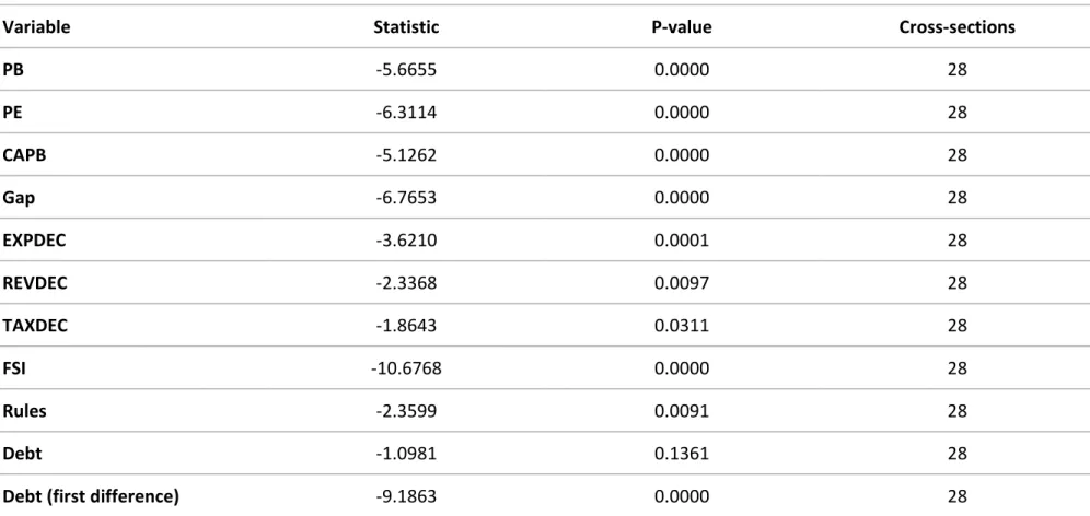
To test the stationarity of the variables, we followed Afonso & Hauptmeier (2009) approach and applied the Im-Pesaran-Shin panel unit root test. The results (stated in Table B. V), indicate that the Debt variable it’s the only one presenting a nonstationary behaviour and therefore, we considered its difference in the model (Baskaran, 2010) since it presented a better outcome on the mentioned test.

4. Empirical Strategy and Results

4.1 Econometric Approach

In this empirical study, the main hypothesis that we want to assess are:

• H1: A higher fiscal rule index (i.e. stronger and wider rules) have a positive influence on the government fiscal policy;

• H2: Higher levels of expenditure decentralization result in better and sustainable budgetary behaviour by the member countries;

• H3: When the member country held parliamentary elections, this event resulted in an expansionary fiscal policy by the government in that year; • H4: An increase in the financial stress is associated to a deterioration of the

fiscal policy stance of the EU member country.

The most common method used to test econometrically the impact of the explanatory variables on the fiscal policy of the government is through the creation of a fiscal reaction function. According with Bohn (1998), a country fiscal policy can be essentially described as the response of the primary balance to three determinants: cyclical fluctuations; past developments in government debt; institutional (political) determinants or temporary events.

18

Therefore, to test the hypothesis previously presented, we estimate the following equation:

(6) 𝐹𝑃𝑆𝑖𝑡 = 𝛼𝑖 + 𝛽1𝛥𝐷𝑒𝑏𝑡𝑖𝑡−1+ 𝛽2𝐺𝑎𝑝𝑖𝑡−1+ 𝛽3𝐸𝑋𝑃𝐷𝐸𝐶𝑖𝑡+ 𝛽4𝐸𝑙𝑒𝑐𝑡𝑖𝑜𝑛𝑖𝑡+

𝛽5𝐹𝑆𝐼𝑖𝑡 + 𝛽6𝑅𝑢𝑙𝑒𝑠𝑖𝑡+ 𝛽7𝐶𝑜𝑛𝑡𝑟𝑜𝑙𝑖𝑡+ 𝜀𝑖𝑡

Where the dependent variable FPS is a proxy for the alternatives measures of the fiscal policy stance (primary balance and primary expense) of the member country i (i = 1, 2, … , 28) and year t (t = 1990, 1991, … , 2017). Whereas the explanatory variables are ΔDebt, Gap, EXPDEC, Election, FSI, Rules and Control. ΔDebt stands for the lagged change in debt-to-GDP ratio (Tagkalakis, 2012), Gap represents the lagged output gap in percentage of the potential GDP, EXPDEC represents the government expenditure decentralization, Election represents a dummy variable for the electoral calendar, FSI the value of the financial stress index and Rules the value of the fiscal rules index. Control represents a set of dummy variables that might have additional explanatory power focused on specific events. α represents the individual effects of each country and ε stands for a time- and country-specific error term.

Considering the absence of data for some variables in certain years and countries (we can perceive this fact by analysing the difference between the number of observations in Table I), it is possible to conclude that we are estimating an unbalanced panel. Furthermore, we can consider our panel dynamic, given that our model uses lagged explanatory variables. Therefore, our panel data assumes a dynamic unbalanced specification (Baltagi, 2005).

19

Based on this consideration, we excluded the LSDVC9 _{method, since it is not}

compatible with an unbalanced panel data. A Breusch and Pagan Lagrangian multiplier test for random effects was performed and its results showed that a random effects model it was not appropriated. Forwardly, we performed the Modified Wald test for groupwise heteroskedasticity in fixed effect regression model and it detected the presence of heteroskedasticity and therefore the need to robust our standard errors. Following Afonso & Guimarães (2014) we adopted a fixed effects estimator in our baseline model.

4.2 Empirical Results

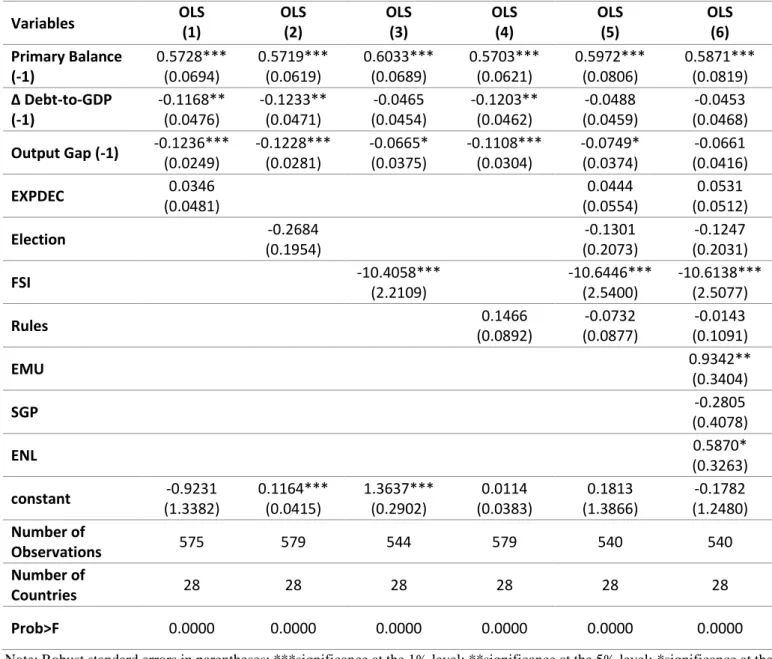
In Table II it is presented the results of the regression based on the fiscal reaction function. Firstly, we used the primary balance as our measure of the fiscal policy stance and regressed it with each one of the variables independently. From columns (1) – (4) of the Table II the results of our regression show that the primary balance is only statistically influenced by the financial stress index, i.e. as the FSI increases by 1 the Primary Balance tend to be affected by -10.4058% of GDP. The relation between these variables supports the idea that in the event of a financial crisis policy makers tend to adjust the fiscal policy to reduce the impact of such incident (Tagkalakis, 2012).

In column (5) all the variables in study are combined in the regression without the control variables for certain events. The results remain the same as the previous ones in terms of statistical significance, with only the FSI presenting a strong statistical connection with the dependent variable, with its coefficient showing a negative relation between the FSI and the PB.

20

According with the results presented in column (6), where all variables are combined (including the event-related ones), it is possible to conclude that once again only the FSI presents a strong statistical relation with the dependent variable. Regarding the event-related dummies, a slightly significant coefficient was obtained for both the EMU and the ENL, which means that the 15 countries that were on the run to the EMU tend to present an improvement in the primary balance as well as the countries that joined the EU afterwards.

Table II - OLS (Fixed Effects) results for the fiscal policy stance (primary balance)

Variables OLS ₍₁₎ OLS ₍₂₎ OLS ₍₃₎ OLS ₍₄₎ OLS ₍₅₎ OLS ₍₆₎ Primary Balance (-1) 0.5728*** (0.0694) 0.5719*** (0.0619) 0.6033*** (0.0689) 0.5703*** (0.0621) 0.5972*** (0.0806) 0.5871*** (0.0819) Δ Debt-to-GDP (-1) -0.1168** (0.0476) -0.1233** (0.0471) -0.0465 (0.0454) -0.1203** (0.0462) -0.0488 (0.0459) -0.0453 (0.0468) Output Gap (-1) -0.1236*** (0.0249) -0.1228*** (0.0281) -0.0665* (0.0375) -0.1108*** (0.0304) -0.0749* (0.0374) -0.0661 (0.0416) EXPDEC 0.0346 (0.0481) 0.0444 (0.0554) 0.0531 (0.0512) Election -0.2684 (0.1954) -0.1301 (0.2073) -0.1247 (0.2031) FSI -10.4058*** (2.2109) -10.6446*** (2.5400) -10.6138*** (2.5077) Rules 0.1466 (0.0892) -0.0732 (0.0877) -0.0143 (0.1091) EMU 0.9342** (0.3404) SGP -0.2805 (0.4078) ENL 0.5870* (0.3263) constant -0.9231 (1.3382) 0.1164*** (0.0415) 1.3637*** (0.2902) 0.0114 (0.0383) 0.1813 (1.3866) -0.1782 (1.2480) Number of Observations 575 579 544 579 540 540 Number of Countries 28 28 28 28 28 28 Prob>F 0.0000 0.0000 0.0000 0.0000 0.0000 0.0000

Note: Robust standard errors in parentheses; ***significance at the 1% level; **significance at the 5% level; *significance at the 10% level

21

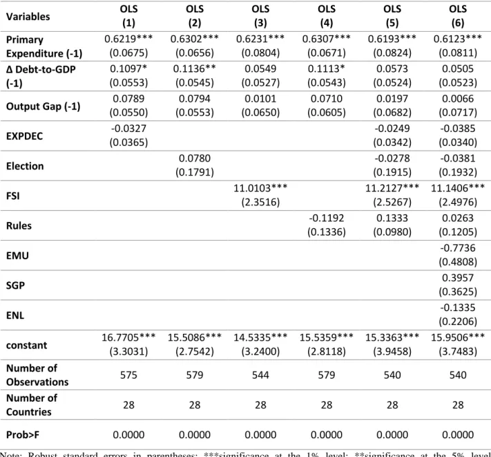
Considering the primary expenditure as our measure for the fiscal policy stance the results of the regression using the same fixed effects estimator are presented in Table III.

Table III - OLS (Fixed Effects) results for the fiscal policy stance (primary expenditure) Variables OLS ₍₁₎ OLS ₍₂₎ OLS ₍₃₎ OLS ₍₄₎ OLS ₍₅₎ OLS ₍₆₎ Primary Expenditure (-1) 0.6219*** (0.0675) 0.6302*** (0.0656) 0.6231*** (0.0804) 0.6307*** (0.0671) 0.6193*** (0.0824) 0.6123*** (0.0811) Δ Debt-to-GDP (-1) 0.1097* (0.0553) 0.1136** (0.0545) 0.0549 (0.0527) 0.1113* (0.0543) 0.0573 (0.0524) 0.0505 (0.0523) Output Gap (-1) _(0.0550) 0.0789 _(0.0553) 0.0794 _(0.0650) 0.0101 _(0.0605) 0.0710 _(0.0682) 0.0197 _(0.0717) 0.0066 EXPDEC _(0.0365) -0.0327 _(0.0342) -0.0249 _(0.0340) -0.0385 Election _(0.1791) 0.0780 _(0.1915) -0.0278 _(0.1932) -0.0381 FSI 11.0103*** _(2.3516) 11.2127*** _(2.5267) 11.1406*** _(2.4976) Rules _(0.1336) -0.1192 _(0.0980) 0.1333 _(0.1205) 0.0263 EMU _(0.4808) -0.7736 SGP _(0.3625) 0.3957 ENL _(0.2206) -0.1335 constant 16.7705*** _(3.3031) 15.5086*** _(2.7542) 14.5335*** _(3.2400) 15.5359*** _(2.8118) 15.3363*** _(3.9458) 15.9506*** _(3.7483) Number of Observations 575 579 544 579 540 540 Number of Countries 28 28 28 28 28 28 Prob>F 0.0000 0.0000 0.0000 0.0000 0.0000 0.0000

In this case, only the FSI variable showed, once again, statistically significant coefficients throughout all regressions in which it was used. Given the fact that the dependent variable is the primary expenditure, the coefficients for the FSI presented a Note: Robust standard errors in parentheses; ***significance at the 1% level; **significance at the 5% level; *significance at the 10% level

22

coherent reversion of the signal. This reversion is explained with the fact that the PE is negatively related with the PB (see equation 7) and therefore the results of the regressions using the PE as dependent variable will present a reversion in the signal of the coefficients.

(7) 𝑃𝑟𝑖𝑚𝑎𝑟𝑦 𝐵𝑎𝑙𝑎𝑛𝑐𝑒 = 𝑅𝑒𝑣𝑒𝑛𝑢𝑒𝑠 − 𝑃𝑟𝑖𝑚𝑎𝑟𝑦 𝐸𝑥𝑝𝑒𝑛𝑑𝑖𝑡𝑢𝑟𝑒𝑠

Regarding the rest of the variables, in most of the cases the reversion of the signal also occurred, however none of the coefficients presented to be statistically significant.

All in all, we were able to find results that support one of the considered hypotheses and reject the others. Indeed, an increase in the financial stress leads to a deterioration of the fiscal policy stance in the EU member country. Therefore, H4 was supported by the results of this study. Regarding the rest of the hypothesis, although the obtained coefficients were consistent with the statement of some of those hypothesis (H2 and H3), there was not enough statistical significance to support a direct relationship between these facts and therefore, reject the rest of the hypothesis.

4.3 Robustness Test

To confirm the outcomes obtained in the baseline model, we performed some robustness tests. Firstly, instead of the use of the primary balance or expenditure as an indicator for the fiscal policy stance we used the cyclically adjusted primary balance (CAPB) following Szymanska (2016) and Ayuso et al. (2008). Forwardly, instead of using

23

the OLS (fixed effects) estimator, we used the 2SLS (IV-FE) estimator given that the first one could present a considerable bias10 _{when used in a dynamic panel regression.}

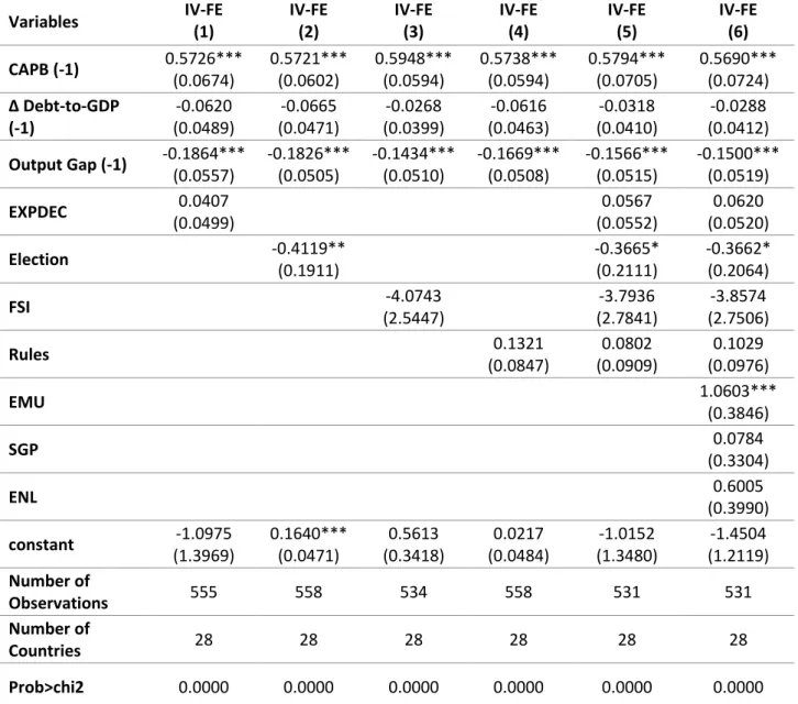
The results of such regression are detailed in Table IV. Overall the outcomes derived from the application of the 2SLS present to be similar to the ones obtained with the OLS using the primary balance as dependent variable. For the EXPDEC variable, it remained statistically insignificant and the obtained coefficients are consistent with the ones obtained in Table II.

The FSI coefficients stated in the columns (3), (5) and (6) show that the relation with the dependent variable remains negative, however they’ve lost their statistical significance. The loss of the statistical significance and the increase of the coefficients might be explained with the fact that the CAPB does not consider the cyclical component of the government budget, resulting in the exclusion of the effects that some temporary events (such as a financial crisis) might have in the balance.

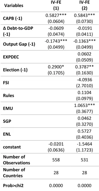
Another difference in terms of statistical significance between the two tested models are the results stated for the variable Election. A slight statistical significance was obtained throughout the three regressions outcomes in which this variable was used. The results obtained in those regressions showed that when parliamentary elections take place the CAPB tend to be negatively affected by around 0.4% in those years. This relation is explained by Nordhaus (1974) that justifies it with the effort that the ruling party does in the pre-electoral period to provide a better condition to the

24

Note: Robust standard errors in parentheses; ***significance at the 1% level; **significance at the 5% level; *significance at the 10% level. Instrumental variables are the t-2 and t-3 lags of the output gap, Tagkalakis (2012)

population, i.e. an expansionary fiscal policy, and with that, increase the chances of re-election.

Table IV - Results for the 2SLS (IV-FE) estimator with CAPB as dependent variable Variables IV-FE ₍₁₎ IV-FE ₍₂₎ IV-FE ₍₃₎ IV-FE ₍₄₎ IV-FE ₍₅₎ IV-FE ₍₆₎ CAPB (-1) 0.5726*** (0.0674) 0.5721*** (0.0602) 0.5948*** (0.0594) 0.5738*** (0.0594) 0.5794*** (0.0705) 0.5690*** (0.0724) Δ Debt-to-GDP (-1) -0.0620 (0.0489) -0.0665 (0.0471) -0.0268 (0.0399) -0.0616 (0.0463) -0.0318 (0.0410) -0.0288 (0.0412) Output Gap (-1) -0.1864*** (0.0557) -0.1826*** (0.0505) -0.1434*** (0.0510) -0.1669*** (0.0508) -0.1566*** (0.0515) -0.1500*** (0.0519) EXPDEC 0.0407 (0.0499) 0.0567 (0.0552) 0.0620 (0.0520) Election -0.4119** (0.1911) -0.3665* (0.2111) -0.3662* (0.2064) FSI -4.0743 (2.5447) -3.7936 (2.7841) -3.8574 (2.7506) Rules 0.1321 (0.0847) 0.0802 (0.0909) 0.1029 (0.0976) EMU 1.0603*** (0.3846) SGP 0.0784 (0.3304) ENL _(0.3990) 0.6005 constant -1.0975 (1.3969) 0.1640*** (0.0471) 0.5613 (0.3418) 0.0217 (0.0484) -1.0152 (1.3480) -1.4504 (1.2119) Number of Observations 555 558 534 558 531 531 Number of Countries 28 28 28 28 28 28 Prob>chi2 0.0000 0.0000 0.0000 0.0000 0.0000 0.0000 4.4 Additional Study

Motivated by the results obtained in the baseline model and in the robustness test we decided to perform further research in the connection of the fiscal policy stance to the decentralization levels and to the electoral cycle.

25

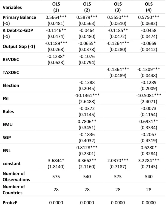
To complement the study on the connection between the decentralization of the government and the fiscal policy stance, we followed Baskaran (2010) and Afonso & Hauptmeier (2009) that also studied the connection of the FPS to the revenues decentralization and to the taxation decentralization. Separated regressions using a fixed effects estimator were performed for each one of these variables given the chance of a high correlation between them. The outcomes (presented in Table A. I) for the revenues decentralization are shown in the columns (1)-(2) and the obtained coefficients show that this kind of decentralization results in a negative impact on the primary balance and therefore in the fiscal policy stance of the EU countries, however due to the weak statistical significance of the obtained coefficients one cannot establish a direct connection between those two events [a similar result was obtained by

Baskaran (2010)]. On the columns (3)-(4) the results of the regression using the taxation decentralization level as an explanatory variable show that a government that ends up in attributing tax responsibilities to sub-national levels of it, tends to present a lower primary balance. This statistically significant result is unexpected, however as it is explained by Baskaran (2010) the decentralization might take the regions to compete and therefore tend to reduce their tax levels to attract companies and individuals to their territory.

Following the outcomes of the robustness test regarding the electoral calendar, we decided to check the hypothesis launched by Nordhaus (1974) who stated that after the elections, governments tend to correct their behaviour of the pre-electoral period. The findings of such connection are shown in Table A. II using a lagged Elections dummy variable. According with the presented results, it is not possible to support Nordhaus

26

(1974) relation given the weakly statistically significant results. However, it is possible to claim that it cannot also be rejected given that in the years immediately after the Parliamentary Elections, the CAPB tended to be higher and therefore policy makers have a tendency to correct their pre-electoral behaviour after the elections period.

5. Conclusion

With the monetary policy exhausted due to the effects of the previous financial crisis, the fiscal policy will have an important role to define the future economic growth of the European Union. It was with this premise that we started this study to analyse which one if not all the four considered variables of the fiscal policy stance have an impact on these policies.

Regarding the financial stress, it was proved that there is a connection between what is happening in the financial markets and the fiscal policy stance. According with the obtained results, policy makers tend to adapt the government economic policy when faced with such event to reduce its impact on the overall economy. Besides, from the outcome of our robustness test, it was proved that most of this adaptation comes from the cyclical component of the public budget.

For the government decentralization, we have not found evidences, given the absence of statistically significant outcomes, that when it is done in the expenditure side of the government budget, the fiscal policy stance tends to improve. However, as we found in our further research, if a government tend to delegate to sub-national authorities the taxation, this decision leads to a deterioration of the CAPB. We can explain such connection with the fact that regions tend to compete to attract companies and individuals to their territory with attractive tax levels.

27

Considering the electoral calendar, we were not able to prove Nordhaus (1974)

results and conclude that a relative austerity is applied in the early years of the mandate, and it ends with expansionary policies before the elections, however one cannot also reject such relation given the obtained outcomes.

Concerning the connection between the application of numerical fiscal rules in the EU member countries and its fiscal policy stance, we were not able to obtain a statistically significant result that prove such relation. This is a subject for which we recommend further research and therefore we would suggest it to future studies. The consideration of different datasets or the application of different regression estimators are some potential paths when approaching such connection. Furthermore, a focus on the partisan model to search for the impact of the ruling party ideology on the fiscal policy it is also recommended.

28

References

Afonso, A., & Guimarães, A. (2014). The relevance of fiscal rules for fiscal and yield developments. Lisboa School of Economics and Management Working Paper, WP05/2014/DE/UECE.

Afonso, A., & Hauptmeier, S. (2009). Fiscal Behaviour in the European Union - Rules, Fiscal decentralization and Government indebtedness. ECB Working Paper Series, 1054.

Alesina, A., & Roubini, N. (1992). Political Business Cycles in OECD Economies. Review of Economic Studies, 59 (4), pp. 663-688.

Ayuso-i-Casals, J. (2012). National Expenditure Rules - Why, How and When. EC Economic Papers, 473.

Ayuso-i-Casals, J., Hernandez, D., Moulin, L., & Turrini, A. (2007). Beyond the SGP: Features and effects of EU national-level fiscal rules. Centre for Economic Policy Research.

Baltagi, B. (2005). Econometric Analysis of Panel Data 3rd Ed. John Wiley & Sons, Ltd. Baskaran, T. (2010). On the link between fiscal decentralization and public debt in

OECD countries. Public Choice 145, pp. 351-378.

Beyer, A., Coeuré, B., & Mendicino, C. (2017). Foreword ‒ The Crisis, Ten Years After: Lessons Learnt for Monetary and Financial Research. ECONOMIE ET

STATISTIQUE / ECONOMICS AND STATISTICS N° 494-495-496.

Bohn, H. (1998). The Behaviour of U.S. Public Debt and Deficits. The Quarterly Journal of Economics, 113 (3), pp. 949-963.

29

de Mello JR, L. (2000). Fiscal Decentralization and Intergovernmental Fiscal Relations: A Cross-Country Analysis. World Development, 28 (2), pp. 365-380.

Debrun, X., Moulin, L., Turrini, A., Ayuso-i-Casals, J., & Kumar, M. (2008). Tied to the mast? National fiscal rules in the European Union. Economic Policy, 23 (54), pp. 297-362.

Döring, Holger and Philip Manow. (2018). Parliaments and governments database (ParlGov): Information on parties, elections and cabinets in modern

democracies. Stable Version. Retrieved from http://www.parlgov.org/

Draghi, M., & de Guindos, L. (2019). Press Conference. Frankfurt am Main: ECB Directorate General Communications. Retrieved from

https://www.ecb.europa.eu/press/pressconf/2019/html/ecb.is190912~658eb5 1d68.en.html#qa

European Central Bank. (2019). Country Level Index of Financial Stress (CLIFS). Retrieved from https://sdw.ecb.europa.eu/browse.do?node=9693347 European Commission. (2019). Fiscal rules database. Retrieved from

https://ec.europa.eu/info/publications/fiscal-rules-database_en

European Commission's Directorate General for Economic and Financial Affairs. (2019). AMECO. Retrieved from

https://ec.europa.eu/economy_finance/ameco/user/serie/SelectSerie.cfm Eurostat. (2019). Government Finance Statistics . Retrieved from

https://ec.europa.eu/eurostat/statistics-explained/index.php?title=Integrated_government_finance_statistics_presenta tion

30

Furceri, D., & Zdzienicka, A. (2010). The consequences of banking crises for public debt. OECD Economic Department Working Papers, 801.

Gujarati, D. (2003). Basic Econometrics 4th Ed. New York: McGraw-Hill.

Horváthová, L., Horváth, J., Gazda, V., & Kubák, M. (2012). Fiscal decentralization and public debt in the European Union. Journal of Local Self-Government, 10 (3), pp. 265-276.

Judson, R., & Owen, A. (1999). Estimating dynamic panel data models: a guide for macroeconomists. Economic Letters, 65, pp. 9-15.

Kopits, G., & Symansky, S. (1998). Fiscal Policy Rules. IMF Occasional Papers, 162. Liew, V. (2004). What lag selection criteria should we employ?. Economics Bulletin,

33(3), pp. 1-9

Nordhaus, W. (1974). The Political Business Cycle. Review of Economic Studies, 42, pp. 169-190.

Oates, W. (1999). An essay on fiscal federalism. Journal of Economic Literature, 37, pp. 1120-1149.

Prud'homme, R. (1995). The dangers of decentralization. The World Bank Research Observer, 10 (2), pp. 201-220.

Stegarescu, D. (2005). Public Sector Decentralisation: Measurement Concepts and Recent International Trends. Fiscal Studies, 26 (3), pp. 301-333.

Szymanska, A. (2016). Effects of fiscal rules on budgetary outcomes: The case of the European Union member states. Acta Oeconomica, 66 (4), pp. 597-616.

Tagkalakis, A. (2012). The effects of financial crisis on fiscal positions. European Journal of Political Economy.

31

The EU Member States. (2008). Protocol (No 12) on the excessive deficit procedure. Official Journal 115, pp. 0279 - 0280.

32

Note: Robust standard errors in parentheses; ***significance at the 1% level; **significance at the 5% level; *significance at the 10% level

Appendix A

Table A. I - OLS (Fixed-Effects) results for decentralization effects on the primary balance

Variables OLS ₍₁₎ OLS ₍₂₎ OLS ₍₃₎ OLS ₍₄₎ Primary Balance (-1) 0.5664*** (0.0481) 0.5879*** (0.0563) 0.5550*** (0.0610) 0.5750*** (0.0682) Δ Debt-to-GDP (-1) -0.1146** (0.0474) -0.0464 (0.0480) -0.1185** (0.0472) -0.0458 (0.0474) Output Gap (-1) -0.1189*** (0.0268) -0.0655* (0.0378) -0.1264*** (0.0280) -0.0669 (0.0412) REVDEC -0.1238* (0.0623) -0.1076 (0.0794) TAXDEC -0.1364*** (0.0489) -0.1309*** (0.0448) Election -0.1288 (0.2045) -0.1289 (0.2009) FSI -10.1361*** (2.6488) -10.5081*** (2.4071) Rules -0.0372 (0.1145) -0.0073 (0.1154) EMU 0.7806** (0.3451) 0.6931** (0.3334) SGP -0.1836 (0.4032) -0.2067 (0.4319) ENL 0.8128*** (0.2301) 0.6280* (0.3284) constant 3.6844* (1.8140) 4.3662** (2.1160) 2.0370*** (0.7187) 3.2284*** (0.7145) Number of Observations 575 540 575 540 Number of Countries 28 28 28 28 Prob>F 0.0000 0.0000 0.0000 0.0000

33

Note: Robust standard errors in parentheses; ***significance at the 1% level; **significance at the 5% level; *significance at the 10% level. Instrumental variables are the t-2 and t-3 lags of the output gap,

Tagkalakis (2012)

Table A. II - Results for the 2SLS (IV-FE) estimator with CAPB as dependent variable and a lagged electoral variable

Variables IV-FE ₍₁₎ IV-FE ₍₂₎ CAPB (-1) 0.5827*** (0.0604) 0.5843*** (0.0730) Δ Debt-to-GDP (-1) -0.0609 (0.0474) -0.0191 (0.0411) Output Gap (-1) -0.1743*** (0.0499) -0.1363*** (0.0499) EXPDEC 0.0602 (0.0509) Election (-1) 0.2900* (0.1705) 0.3787** (0.1630) FSI -4.0936 (2.7010) Rules 0.1104 (0.0979) EMU 1.0653*** (0.3677) SGP 0.0462 (0.3270) ENL 0.5727 (0.4036) constant -0.0201 (0.0636) -1.5464 (1.1723) Number of Observations 558 531 Number of Countries 28 28 Prob>chi2 0.0000 0.0000

34

Appendix B

Graph B. I – Evolution of the number of numerical fiscal rules by type

Graph B. II – Weight of each type of rule per government coverage Source: European Commission

35

Graph B. III – Evolution of the FSI for France, 1990 - 2017

Graph B. IV – Evolution of the FSI for Germany, 1990 - 2017

Source: European Central Bank

36

Graph B. V – Evolution of the FSI for Greece, 1990 - 2017

Graph B. VI – Evolution of the FSI for Ireland, 1990 - 2017

Source: European Central Bank

37

Graph B. VII – Evolution of the FSI for Portugal, 1990 - 2017

Graph B. VIII – Evolution of the FSI for Spain, 1990 - 2017

Source: European Central Bank

38

Graph B. IX – Evolution of the FSI for United Kingdom, 1990 - 2017

39

Table B. I - Codes of the variables collected from AMECO

Variable Name AMECO Code

Primary Balance UBLGI

Primary Expenditure UUTGI

Debt-to-GDP UDGG

Output Gap AVGDGP

Cyclically Adjusted Primary Balance UBLGBP

Table B. II - Results obtained in (1) for every EU member country, %

REVDEC EXPDEC TAXDEC

1995 2005 2010 2015 1995 2005 2010 2015 1995 2005 2010 2015 Austria 36.39 34.10 34.70 35.00 33.58 32.61 34.17 34.06 7.87 6.09 6.31 6.02 Belgium 41.63 44.01 45.38 49.03 39.23 41.47 43.63 49.06 10.56 15.01 15.74 19.17 Bulgaria 28.67 20.38 22.67 25.85 27.78 22.25 21.33 27.20 16.33 2.56 3.88 4.06 Croatia 30.79 32.51 30.78 28.68 27.45 28.46 15.35 18.25 17.40 Cyprus 4.63 6.27 6.53 5.21 4.37 5.66 5.41 4.92 2.06 1.69 1.92 2.00 Czech Republic 32.70 29.82 30.57 28.91 22.25 27.95 28.69 27.09 19.88 25.74 25.01 25.20 Denmark 46.08 45.12 47.37 47.10 43.60 48.92 45.85 45.98 31.32 30.56 26.71 25.95 Estonia 21.72 23.23 22.86 21.83 22.03 24.52 22.14 21.23 1.21 1.79 2.27 1.52 Finland 44.96 41.82 49.09 47.52 35.02 42.80 44.16 45.39 32.36 28.50 34.60 33.55 France 29.95 33.37 36.37 36.71 27.15 31.10 31.07 33.05 19.95 21.46 21.59 26.64 Germany 59.56 61.22 60.78 62.06 50.54 58.75 56.62 62.71 48.24 49.52 48.44 50.87 Greece 11.16 10.32 10.89 9.42 7.96 8.27 8.83 7.67 3.04 3.40 3.62 3.42 Hungary 31.13 32.47 28.35 19.57 25.56 28.16 27.32 18.27 10.27 17.53 9.57 8.86 Ireland 26.55 16.42 14.81 8.72 25.56 16.58 7.88 7.44 2.73 2.34 3.52 2.73 Italy 29.63 38.55 37.94 36.33 25.26 36.39 35.13 33.15 11.49 22.79 21.30 21.86 Latvia 30.68 31.29 35.16 30.64 27.93 30.09 30.56 28.25 30.38 23.54 29.25 26.21 Lithuania 24.48 24.91 32.08 25.93 23.42 24.37 28.36 24.71 3.05 2.11 3.01 2.25 Luxembourg 16.88 14.29 15.27 13.80 16.53 14.59 13.95 12.70 8.70 6.17 6.12 4.89 Malta 1.64 1.50 1.71 1.50 1.41 1.36 1.48 1.31 0.00 0.00 0.00 0.00 Netherlands 45.73 35.90 36.19 35.58 38.94 36.43 34.74 34.30 5.27 6.16 5.80 6.22 Poland 23.80 37.81 38.81 38.31 25.58 34.03 35.24 36.04 12.24 20.22 19.28 21.10 Portugal 15.25 17.33 18.80 16.87 13.15 15.44 15.98 13.86 7.53 9.33 9.50 10.12 Romania 17.08 23.00 28.81 29.72 15.04 22.43 24.50 26.98 12.78 4.78 5.94 4.92 Slovakia 10.04 22.78 23.33 22.05 15.96 20.85 20.86 20.22 6.28 3.85 4.35 2.92 Slovenia 23.36 23.48 27.15 24.81 18.64 22.29 24.24 22.27 11.11 11.67 18.15 15.85 Spain 43.04 52.57 55.98 53.50 37.95 53.68 54.30 51.45 21.10 33.49 34.92 35.86 Sweden 42.23 42.31 43.90 44.78 37.61 42.24 43.42 45.29 33.66 34.45 32.87 32.83 United Kingdom 24.19 24.42 26.95 23.00 22.32 23.70 22.85 21.18 4.49 5.66 6.08 5.88

40

Table B. III – Correlation Matrix

PB PE CAPB Debt Gap EXPDEC Election FSI Rules EMU SGP ENL PB 1 PE -0.1956 1 CAPB 0.8803 -0.0323 1 Debt -0.029 0.2995 0.1605 1 Gap 0.3534 -0.3284 -0.1258 -0.3602 1 EXPDEC 0.2225 0.3853 0.2331 -0.0264 0.0147 1 Election -0.0475 0.0053 -0.0615 0.0057 0.0154 0.0131 1 FSI -0.3368 0.1612 -0.2108 0.0229 -0.2895 -0.0527 0.0419 1 Rules 0.1671 0.0518 0.2547 0.0418 -0.1353 0.3004 0.0246 -0.2085 1 EMU 0.1631 0.0308 0.1913 0.0895 -0.0242 0.0522 -0.0211 -0.031 -0.2165 1 SGP 0.0379 0.1581 0.0895 0.3847 -0.0929 0.0805 0.016 0.0646 0.2039 -0.3173 1 ENL -0.1531 -0.3176 -0.1902 -0.2613 0.0373 -0.2825 0.0123 -0.0187 0.0303 -0.2066 -0.2329 1

41

Table B. IV - Averages of all variables per country

PB PE CAPB Debt Gap EXPDEC REVDEC TAXDEC Elections FSI Rules EMU SGP ENL

Austria 0.464 48.704 0.588 72.568 -0.121 33.503 34.876 6.401 0.321 0.123 0.084 0.143 0.679 0.000 Belgium 2.940 46.792 2.901 105.799 0.083 42.986 44.566 14.750 0.250 0.142 0.255 0.143 0.679 0.000 Bulgaria 1.948 34.309 1.834 36.756 0.381 22.315 22.582 8.170 0.321 0.124 0.366 0.000 0.000 0.393 Croatia -1.514 45.109 -1.371 54.913 -0.322 28.483 31.070 17.032 0.214 0.098 -0.564 0.000 0.000 0.179 Cyprus -0.180 35.531 -0.095 67.900 -0.022 4.802 5.416 1.921 0.214 0.101 -0.450 0.000 0.357 0.500 Czech Republic -2.238 41.787 -1.843 28.454 0.064 26.809 29.253 23.234 0.321 0.141 -0.864 0.000 0.000 0.500 Denmark 2.931 51.458 2.953 41.354 -0.432 46.350 46.060 28.946 0.286 0.111 0.518 0.143 0.000 0.000 Estonia 0.510 37.765 0.496 6.819 0.029 22.935 22.274 1.885 0.250 0.138 0.942 0.000 0.250 0.500 Finland 1.951 51.813 2.481 46.015 -0.911 42.489 44.011 31.146 0.250 0.192 0.348 0.143 0.679 0.000 France -0.995 51.497 -0.808 73.891 -0.300 30.785 33.965 22.714 0.214 0.125 -0.201 0.143 0.679 0.000 Germany 0.563 43.687 0.557 66.493 0.012 59.744 61.130 49.833 0.286 0.126 0.321 0.143 0.679 0.000 Greece -1.368 43.188 0.055 127.491 -1.851 8.539 10.867 3.349 0.321 0.161 -0.635 0.143 0.607 0.000 Hungary -0.030 44.504 -0.042 68.472 -0.484 24.614 28.078 12.610 0.250 0.151 -0.656 0.000 0.000 0.500 Ireland -0.556 34.579 -0.923 60.999 0.549 18.907 19.408 2.647 0.214 0.198 -0.459 0.143 0.679 0.000 Italy 2.291 43.181 2.585 110.668 -0.511 33.413 35.667 20.087 0.250 0.130 0.114 0.143 0.679 0.000 Latvia -1.050 36.359 -0.940 23.419 -0.340 31.221 32.896 26.145 0.321 0.110 -0.266 0.000 0.143 0.500 Lithuania -1.775 36.271 -1.691 25.882 -0.277 25.166 26.778 2.520 0.286 0.106 0.124 0.000 0.107 0.500 Luxembourg 2.263 41.229 2.498 13.359 -0.114 14.726 15.308 6.788 0.179 0.151 0.107 0.143 0.679 0.000 Malta -0.781 38.093 -0.733 60.475 -0.101 1.436 1.634 0.000 0.250 0.125 -0.569 0.000 0.357 0.500 Netherlands 0.579 42.412 1.034 58.019 -0.477 35.481 36.414 5.800 0.286 0.101 0.855 0.143 0.679 0.000 Poland -1.255 41.512 -1.021 46.664 -0.469 33.468 35.987 18.286 0.286 0.111 0.384 0.000 0.000 0.500 Portugal -1.415 42.388 -1.217 82.299 0.083 15.259 17.220 9.101 0.286 0.105 -0.148 0.143 0.679 0.000 Romania -1.238 34.045 -1.218 23.810 -0.061 21.988 24.398 7.015 0.286 0.136 -0.189 0.000 0.000 0.393 Slovakia -2.590 40.985 -2.633 41.273 -0.073 17.134 18.567 5.217 0.321 0.105 0.036 0.000 0.321 0.500 Slovenia -1.506 44.781 -1.281 39.027 -0.417 22.398 24.482 13.978 0.286 0.135 -0.768 0.000 0.393 0.500 Spain -0.978 38.987 -0.256 64.701 -1.071 49.471 51.538 32.125 0.286 0.126 0.565 0.143 0.679 0.000 Sweden 2.133 51.003 2.491 48.983 -0.929 43.018 42.839 33.767 0.250 0.134 0.676 0.143 0.000 0.000 United Kingdom -1.342 37.624 -1.130 54.590 -0.385 22.827 24.086 5.464 0.250 0.119 0.102 0.143 0.000 0.000

42

Table B. V – Summary of Im-Pesaran-Shin panel unit root test

Variable Statistic P-value Cross-sections

PB -5.6655 0.0000 28 PE -6.3114 0.0000 28 CAPB -5.1262 0.0000 28 Gap -6.7653 0.0000 28 EXPDEC -3.6210 0.0001 28 REVDEC -2.3368 0.0097 28 TAXDEC -1.8643 0.0311 28 FSI -10.6768 0.0000 28 Rules -2.3599 0.0091 28 Debt -1.0981 0.1361 28

Debt (first difference) -9.1863 0.0000 28